AbstractâA multiresolution frequency domain (MRFD) analysis similar to the finite difference frequency domain (FDFD) method is presented. This new method ...
Progress In Electromagnetics Research, PIER 69, 55–66, 2007
THE MULTIRESOLUTION FREQUENCY DOMAIN METHOD FOR GENERAL GUIDED WAVE STRUCTURES M. Gokten Department of Electrical Engineering and Computer Science Syracuse University Syracuse, NY 13244, USA A. Z. Elsherbeni Department of Electrical Engineering University of Mississippi University, MS 38677, USA E. Arvas Department of Electrical Engineering and Computer Science Syracuse University Syracuse, NY 13244, USA Abstract—A multiresolution frequency domain (MRFD) analysis similar to the finite difference frequency domain (FDFD) method is presented. This new method is derived by the application of MoM to frequency domain Maxwell’s equations while expanding the fields in terms of biorthogonal scaling functions. The dispersion characteristics of waveguiding structures are analyzed in order to demonstrate the advantages of this proposed MRFD method over the traditional FDFD scheme.
1. INTRODUCTION Over the last decade, multiresolution analysis techniques have successfully been applied to various computational electromagnetic methods yielding significant computational CPU and memory savings, compared to the traditional techniques. Multiresolution analysis
56
Gokten, Elsherbeni, and Arvas
has found application in the improvement of method of moments (MoM) [1–4], finite difference time domain (FDTD) method [5–9] and transmission line matrix (TLM) method [10]. The finite difference frequency domain method, on the other hand, has not yet benefited from the advantages of multiresolution analysis. In this paper, we formulate a 3D frequency domain numerical method based on multiresolution analysis from which a special case leads to the FDFD method. It was observed in [5] that the FDTD scheme can be derived by applying MoM to Maxwell’s curl equations while using pulse functions as a basis for the expansion of unknown fields. It is also possible to show that the previous statement is true for FDFD scheme. Since pulse functions are also the scaling functions of the Haar wavelet bases, FDFD scheme can also be considered as multiresolution analysis scheme based only on the scaling function and can be improved by adding Haar wavelet functions to the expansion of the fields. One can further improve the method by using the Cohen-Daubechies-Feauveau (CDF) family of wavelets, which is the focus of this work. 2. FORMULATION 2.1. Wavelet Selection In order to develop an efficient MRFD formulation, one should choose the appropriate wavelet family from an ever-increasing number of wavelets available. For an effective MRFD algorithm, the appropriate wavelet base should have certain properties; such as compact support, symmetry, interpolation property, regularity (smoothness) and maximum number of vanishing moments. The support of the wavelet basis is directly related to the number of terms in the field components update equations. Since a great number of terms in each update equation will increase the computational burden and complicate the coding process, it is preferable to have a compactly supported wavelet base. Symmetric wavelet functions will ensure the symmetry of the formulation and in return will simplify the modeling of symmetry and boundary planes [11]. Compact support and symmetry are incompatible aspects of orthogonal wavelet systems, with the Haar wavelets being the exception. A biorthogonal wavelet base can sustain smooth, compact and symmetric wavelets, which is the main reason for the choice of biorthogonal wavelets over orthogonal ones. In a wavelet expansion, the field value at a certain point is generally reconstructed by a weighted sum of related neighboring basis function coefficients, which requires a complex reconstruction
Progress In Electromagnetics Research, PIER 69, 2007
57
algorithm. However, the reconstruction algorithm is not essential if the basis function satisfies the interpolation property, as in such cases the basis function coefficients represent the field components at the corresponding position of the grid [12]. Thus, a basis function equipped with the interpolation property will not use the weighted sum and thus yields a more efficient MRFD algorithm. Two of the most desired properties of a wavelet family are high regularity and maximum number of vanishing moments, owing to their great effect on how well the wavelet expansion approximates a smooth function. Unfortunately, wavelets do not accommodate both high regularity and high number of vanishing moments concurrently and it is unclear which property is more important [13–14]. Biorthogonal wavelets have two dual scaling functions, which can have different regularity properties. It is mentioned in [13] that, it is useful to reserve the high regularity to the synthesis scaling function and maximum vanished moments to the analysis scaling function. Considering all the requirements mentioned above, CohenDaubechies-Feauveau family of wavelets [13], in particular CDF(2, 2) wavelet, is adopted for this work due to its minimal support. 2.2. 3D Formulation In this section, derivation of the new method for lossless simple media is presented. As an example, we can consider one of Maxwell’s timeharmonic scalar equations: jwεEx (x, y, z) =
∂Hz (x, y, z) ∂Hy (x, y, z) − . ∂y ∂z
(1)
The field components on a Yee cell may be approximated in terms of basis functions as � Ex (i, j, k)φ�i+1/2 (x)φ�j (y)φ�k (z) (2a) Ex (x, y, z) = i,j,k
Hy (x, y, z) =
�
Hy (i, j, k)φ�i+1/2 (x)φ�j (y)φ�k+1/2 (z)
(2b)
Hz (i, j, k)φ�i+1/2 (x)φ�j+1/2 (y)φ�k (z)
(2c)
i,j,k
Hz (x, y, z) =
� i,j,k
Here, the indexes i, j, k indicate the discrete space lattice related to the space grid through x = i∆x, y = j∆y and z = k∆z. The function φ�n (x) is the scaled and shifted CDF dual scaling function � (φ(x)) defined as:
58
Gokten, Elsherbeni, and Arvas
� � x − n∆x φ�n (x) = φ� ∆x
(3)
The field expansions are inserted into (1) and both sides are tested with the scaling function according to Galerkin’s method. During the sampling process, the following integrals are used: �∞ −∞
na � � � ∂ φ�i� +1/2 (y) a(l) δi+l−1,i� − δi−l,i� φi (y)dy = ∂y
(4)
l=1
�∞
φi� (x)φ�i (x)dx = ∆xδi,i�
(5)
−∞
where na is the stencil size and δi,i� is the kronecker delta given by 1, i = i� . (6) δi,i� = 0, i �= i� Stencil sizes and a(l) coefficients of different CDF wavelets are given in [7]. For CDF(2, 2) wavelet, stencil size is 3 and a(l) coefficients are listed in Table 1. Table 1. The a(l) coefficients. l a(l)
1 1.2291667
2 −0.0937500
3 0.0104167
We can now continue the derivation by testing the left-hand side of (1) according to MoM, such that �∞ �∞ �∞ jwε
Ex (x, y, z)φi+1/2 (x)φj (y)φk (z)dxdydz
−∞ −∞ −∞ �∞ �∞ �∞
= jwε −∞ −∞ −∞
� Ex (i, j, k)φ�i+1/2 (x)φ�j (y)φ�k (z) i,j,k
φi+1/2 (x)φj (y)φk (z)dxdydz = jwεEx (i, j, k)∆x∆y∆z
(7)
Progress In Electromagnetics Research, PIER 69, 2007
59
where φn (x) is the scaled and shifted CDF scaling function (φ(x)) defined similar to (3). Testing the first term of the right-hand side of (1) yields: �∞ �∞ �∞
∂Hz (x, y, z) φi+1/2 (x)φj (y)φk (z)dxdydz ∂y −∞ −∞ −∞ �∞ �∞ �∞ � ∂ = Hz (i, j, k)φ�i+1/2 (x)φ�j+1/2 (y)φ�k (z) ∂y i,j,k
−∞ −∞ −∞
φi+1/2 (x)φj (y)φk (z)dxdydz na � = ∆x∆z a(l) [Hz (i, j + l − 1, k) − Hz (i, j − l, k)] .
(8)
l=1
Testing the second term of the right-hand side of (1) similarly yields: �∞ �∞ �∞
∂Hy (x, y, z) φi+1/2 (x)φj (y)φk (z)dxdydz = ∂z
−∞ −∞ −∞ na �
∆x∆y
a(l) [Hy (i, j, k + l − 1) − Hy (i, j, k − l)] .
(9)
l=1
Equating (1), (7), (8) and (9) results in the MRFD update equation: na � a(l) [Hz (i, j + l − 1, k) − Hz (i, j − l, k)] 1 l=1 Ex (i, j, k) = jwε ∆y na �
a(l) [Hy (i, j, k + l − 1) − Hy (i, j, k − l)] . (10) − l=1 ∆z The remaining five update equations, which are not listed here due to space saving considerations, can be derived similarly by applying the same procedure to the rest of the scalar Maxwell’s equations.
60
Gokten, Elsherbeni, and Arvas
2.3. 2D Formulation The determination of the dispersion characteristics of waveguiding structures is a fundamental problem in microwave engineering applications. Furthermore, these characteristics (propagation constant, mode patterns, characteristic impedance, etc.) can be used as port data for 3D simulation of microwave devices [15]. Since such problems are well-suited for frequency domain techniques, characterization of guided wave structures is considered for validation of the proposed method. The eigen-based finite difference frequency domain method was proposed to solve the propagation characteristics of guided wave structures [16]. For the MRFD solution of the problem, a similar approach is adopted. Assuming that the waveguiding structure is uniform along z axis and the wave propagates in positive z direction, the electric and magnetic fields inside guided wave structure can be expressed as: � x + Ey (x, y)ˆ y + Ez (x, y)ˆ z ] e−jβz E(x, y, z) = [Ex (x, y)ˆ � x + Hy (x, y)ˆ y + Hz (x, y)ˆ z ] e−jβz H(x, y, z) = [Hx (x, y)ˆ
(11a) (11b)
where β is the propagation constant. Time harmonic Maxwell’s equations for simple dielectric media are: � = −jωµH, ∇×E � = 0, ∇·D
� = jωεE ∇×H � =0 ∇·B
(12a) (12b)
in which the space derivatives with respect to z can be replaced by −jβ (i.e., ∂/∂z = −jβ). Inserting (11) into (12) yields the following scalar equations: ∂Ez ∂x ∂Ez −wµx Hx + j ∂y ∂Hz −wεy Ey + j ∂x ∂Hz wεx Ex + j ∂y ∂Ey ∂Ex −jεx − jεy ∂x ∂y ∂Hy ∂Hx −jµx − jµy ∂x ∂y
βEx = wµy Hy + j
(13a)
βEy =
(13b)
βHx = βHy = βEz = βµz Hz =
(13c) (13d) (13e) (13f)
Progress In Electromagnetics Research, PIER 69, 2007
61
Note that (13a)–(13d) is derived from Maxwell’s curl equations (12a) and (13e), (13f) is derived from Maxwell’s divergence equations (12b).
Ey Ez
Ex Hy
Hz
Hx
Figure 1. The compact 2D lattice. Equation (13) can be discretized by using the compact 2D Yee cell [16–18] shown in Fig. 1. Two of the resulting update equations are presented below as an example: j � a(l) [Ez (i+l, j)−Ez (i−l+1, j)] ∆x 3
βEx (i, j) = wµy (i, j)Hy (i, j)+
l=1
(14a) βEz (i, j) =
j ∆xεz (i, j)
3 �
a(l)
l=1
[εx (i−l, j)Ex (i−l, j)−εx (i+l−1, j)Ex (i+l−1, j)] 3 � j a(l) + ∆yεz (i, j) l=1
[εy (i, j −l)Ey (i, j −l)−εy (i, j +l−1)Ey (i, j +l−1)]
(14b)
62
Gokten, Elsherbeni, and Arvas
Field update equations can be used to form an eigenvalue problem as: [A] − β[I] · x = 0
(15)
where [A] is a sparse coefficient matrix, [I] is the unit matrix and x is the unknown field vector. The eigen solution of [A] delivers the propagation constant and corresponding electromagnetic fields. 3. NUMERICAL RESULTS First, a dielectric filled rectangular waveguide with dimensions a = 1.5 cm, b = 0.6 cm and relative dielectric constant εr = 2.25, as illustrated in Fig. 2(a), is considered. The propagation constants of the first two higher order modes are computed using the FDFD [16] and the MRFD methods. Results are compared in Fig. 3(a) to the analytical calculations [19]. The convergence of the calculated error with respect to cell size for each method is provided in Fig. 4.
b
b h a
a
(a)
(b)
w
x
b h a
z
y
(c)
Figure 2. Waveguiding structures: (a) dielectric filled waveguide, (b) partially filled waveguide, (c) microstrip line. The second example is a partially filled waveguide as shown in Fig. 2(b). Waveguide dimensions are a = 1.5 cm, b = 0.6 cm and h = 0.3 cm and the relative dielectric constant of the substrate is εr = 2.25. Computed results are given in Fig. 3(b). Finally, the propagation characteristics of a boxed microstrip line (Fig. 2(c)) are considered. The dimensions are a = 1.5 cm, b = 1.5 cm, h = 0.3 cm and w = 0.3 cm and εr of the substrate is 30. The computed effective dielectric constant of this structure is shown in Fig. 5.
Progress In Electromagnetics Research, PIER 69, 2007
63
Propagation Constant [rad/m]
600 500
Analytical FDFD MRFD
400 300 200 100 0 6
TE 01 Mode
8
TE 02 Mode
10
12
14
16
18
20
Frequency [GHz] (a)
Propagation Constant [rad/m]
500 400
Analytical FDFD MRFD
300
200
100
0 8
TM X01 Mode
10
12
TM X02 Mode
14
16
18
20
Frequency [GHz]
(b)
Figure 3. Propagation constant of the first two propagating modes of a waveguide: (a) dielectric filled, (b) partially filled. For all three cases, the MRFD grid was chosen to be coarser than the FDFD grid, yet the accuracy of both methods remained identical. Coarser grid results smaller matrix sizes, reduced computation time and memory requirements. The efficiency of the new method is compared to FDFD in Table 2. Results show that the accuracy of the MRFD method matches that of FDFD method despite savings in terms of memory and in execution time. The memory requirements and execution time of both methods for each example is summarized Table 2. These calculations are performed by MATLAB codes and run on a Windows based personal computer with 3 GB memory and two 600-MHZ Pentium III CPUs.
64
Gokten, Elsherbeni, and Arvas
Table 2. Computer resources consumed by the two methods. Matrix Size [byte] 32336 4384 32336 11600 32336 26620
Mesh size Uniform Waveguide Partially Filled Waveguide Microstrip Line
15 × 6 5×2 15 × 6 5×4 15 × 6 10 × 4
FDTD MRFD FDTD MRFD FDTD MRFD
Time [sec] 1.549 0.268 3.001 0.7433 1.424 0.925
Figure 4. Error convergence of the propagation constant.
Effective Dielectric Constant
30 25 20 15 MRFD FDFD MW Studio
10 5 0
2
3
4
5
6
7
8
9
10
Frequency [GHz]
Figure 5. Effective dielectric constant of the boxed microstrip line.
Progress In Electromagnetics Research, PIER 69, 2007
65
4. CONCLUSION The multiresolution frequency domain scheme based on the biorthogonal CDF wavelet family is developed. The newly developed method together with traditional FDFD method is used to analyze the propagation characteristics of general guided wave structures. Results indicate substantial savings in terms of execution time and memory requirements. It is expected that the savings will be more significant in three dimensional problems. REFERENCES 1. Steinberg, B. Z. and Y. Leviatan, “On the use of wavelet expansions in the method of moments,” IEEE Trans. Antennas Propagat., Vol. 41, 610–619, May 1993. 2. Sabetfakhri, K. and L. P. B. Katehi, “Analysis of integrated millimeter-wave and submillimeter-wave waveguides using orthonormal wavelet expansions,” IEEE Trans. Microwave Theory Tech., Vol. 42, 2412–2422, Dec. 1994. 3. Wagner, R. L. and W. C. Chew, “Study of wavelets for the solution of electromagnetic integral equations,” IEEE Trans. Antennas and Propagat., Vol. 43, 802–810, Aug. 1995. 4. Wei, X. C. and E. P. Li, “Fast solution for large scale electromagnetic scattering problems using wavelet transform and its precondition,” Progress In Electromagnetics Research, PIER 38, 253–267, 2002. 5. Krumpholz, M. and L. P. B. Katehi, “MRTD: new timedomain schemes based on multiresolution analysis,” IEEE Trans. Microwave Theory Tech., Vol. 44, 555–571, Apr. 1996. 6. Fujii, M. and W. J. R. Hoefer, “A three-dimensional Haar-waveletbased multiresolution analysis similar to the FDTD method — derivation and application,” IEEE Trans. Microwave Theory Tech., Vol. 46, 2463–2475, Dec. 1998. 7. Dogaru, T. and L. Carin, “Multiresolution time-domain using CDF biorthogonal wavelets,” IEEE Trans. Microwave Theory Tech., Vol. 49, 902–912, May 2001. 8. Fujii, M. and W. J. R. Hoefer, “A wavelet formulation of the finite-difference method: Full-vector analysis of optical waveguide junctions,” IEEE J. Quantum Electron., Vol. 37, 1015–1029, Aug. 2001. 9. Cao, Q., K. K. Tamma, P. K. A. Wai, and Y. Chen, “RCS scattering analysis using the three-dimensional MRTD scheme,”
66
10.
11. 12.
13. 14.
15.
16.
17.
18.
19.
Gokten, Elsherbeni, and Arvas
J. of Electromagn. Waves and Appl., Vol. 17, No. 12, 1683–1701, 2003. Barba, I., J. Represa, M. Fujii, and W. J. R. Hoefer, “Multiresolution 2D-TLM technique using Haar wavelets,” IEEE MTT-S Int. Microwave Symp. Dig., 243–246, 2000. Pan, G. W., Wavelets in Electromagnetics and Device Modeling, John Wiley & Sons Inc., Hoboken, New Jersey, 2003. Zhu, X., T. Dogaru, and L. Carin, “Analysis of the CDF biorthogonal MRTD method with application to PEC targets,” IEEE Trans. Microwave Theory Tech., Vol. 51, 2015–2022, September 2003. Daubechies, I., Ten Lectures on Wavelets, Society for Industrial and Applied Mathematics, Philadelphia, PA, 1992. Tretiakov, Y., S. Ogurtsov, and G. Pan, “On samplingbiorthogonal time-domain scheme based on daubechies compactly supported wavelets,” Progress In Electromagnetics Research, PIER 47, 213–234, 2004. Pereda, J. A., A. Vegas, L. F. Velarde, and O. Gonzalez, “An FDFD eigenvalue formulation for computing port solutions in FDTD simulators,” Microwave and Opt. Tech. Letters, Vol. 45, 1–3, Apr. 2005. Lui, M. L. and Z. Chen, “A direct computation of propagation constant using compact 2-D full-wave eigen-based finite-difference frequency-domain technique,” Int. Conf. on Comp. Electromagnetics and Its Applications, Beijing, China, 1999. Asi, A. and L. Shafai, “Dispersion analysis of anisotropic inhomogeneous waveguides using compact 2D-FDTD,” Electronics Letters, Vol. 28, 1451–1452, 1992. Cangellaris, A. C., “Numerical stability and numerical dispersion of a compact 2-D/FDTD method used for the dispersion analysis of waveguides,” IEEE Microwave and Guided Wave Letters, Vol. 3, 3–5, 1993. Harrington, R. F., Time-harmonic Electromagnetic Fields, McGraw-Hill Book Company, Inc., York, PA, 1961.