Princeton University Technical Report TR-811-08, January 2008
The PARSEC Benchmark Suite: Characterization and Architectural Implications Christian Bienia† , Sanjeev Kumar‡ , Jaswinder Pal Singh† and Kai Li† †
Department of Computer Science, Princeton University
‡
Microprocessor Technology Labs, Intel
[email protected]
ABSTRACT
suites often include proprietary code and are not publicly available. To address this problem, we created the PARSEC benchmark suite in collaboration with Intel Corporation. It includes not only a number of important applications from the RMS suite but also several leading-edge applications from Princeton University, Stanford University and the open-source domain. The goal is to create a suite of emerging workloads that can drive CMP research.
This paper presents and characterizes the Princeton Application Repository for Shared-Memory Computers (PARSEC), a benchmark suite for studies of Chip-Multiprocessors (CMPs). Previous available benchmarks for multiprocessors have focused on high-performance computing applications and used a limited number of synchronization methods. PARSEC includes emerging applications in recognition, mining and synthesis (RMS) as well as systems applications which mimic large-scale multi-threaded commercial programs. Our characterization shows that the benchmark suite is diverse in working set, locality, data sharing, synchronization, and off-chip traffic. The benchmark suite has been made available to the public.
This paper makes three contributions: • We identify shortcomings of commonly used benchmark suites and explain why they should not be used to evaluate CMPs.
Categories and Subject Descriptors
• We present and characterize PARSEC, a new benchmark suite for CMPs that is diverse enough in order to allow representative conclusions.
D.0 [Software]: [benchmark suite]
General Terms
• Based on our characterization of PARSEC, we analyze what properties future CMPs must have in order to be able to deliver scalable performance for emerging applications. In particular, our understanding of the behavior of future workloads allows us to quantify how CMPs must be built in order to mitigate the effects of the memory wall on the next generation of programs.
Performance, Measurement, Experimentation
Keywords benchmark suite, performance measurement, multi-threading, shared-memory computers
1.
INTRODUCTION
Benchmarking is the quantitative foundation of computer architecture research. Program execution time is the only accurate way to measure performance[18]. Without a program selection that provides a representative snapshot of the target application space, performance results can be misleading and no valid conclusions may be drawn from an experiment outcome. CMPs require a disruptive change in order for programs to benefit from their full potential. Future applications will have to be parallel, but due to the lack of a representative, multi-threaded benchmark suite most scientists were forced to fall back to existing benchmarks. This usually meant the use of older High-Performance Computing (HPC) workloads, smaller suites with only few programs or unparallelized benchmarks. We consider this trend extremely dangerous for the whole discipline. Representative conclusions require representative experiments and, as we argue in this paper, existing benchmark suites cannot be considered adequate to describe future CMP applications.
In Section 2 we describe why existing benchmark suites cannot be considered adequate to describe future CMP applications. In Section 3, we present the PARSEC benchmark suite and explain how it avoids the shortcomings of other collections of benchmarks. The methodology which we use to characterize our workloads is presented in Section 4. In Sections 5 to 8, we analyze the parallelization, working sets, communication behavior and off-chip traffic of the benchmark programs. We conclude our study in Section 9.
2.
MOTIVATION
The goal of this work is to define a benchmark suite that can be used to design the next generation of processors. In this section, we first present the requirements for such a suite. We then discuss how the existing benchmarks fail to meet these requirements.
2.1
Large processor manufacturers have already reacted and developed their own, internal collections of workloads. An example is the Intel RMS benchmark suite[14]. However, these
Requirements for a Benchmark Suite
We have the following five requirements for a benchmark suite: 1
Princeton University Technical Report TR-811-08, January 2008 Multi-threaded Applications Shared-memory CMPs are already ubiquitous. The trend for future processors is to deliver large performance improvements through increasing core counts on CMPs while only providing modest serial performance improvements. Consequently, applications that require additional processing power will need to be parallel.
for example implements the Barnes-Hut algorithm for N-body simulation[8]. For galaxy simulations it has largely been superseded by the TreeSPH[19] method, which can also account for mass such as dark matter which is not concentrated in bodies. However, even for pure N-body simulation barnes must be considered outdated. In 1995 Xu proposed a hybrid algorithm which combines the hierarchical tree algorithm and the Fourier-based Particle-Mesh (PM) method to the superior TreePM method[45]. Our analysis shows that similar issues exist for a number of other applications of the suite including raytrace and radiosity.
Emerging Workloads Rapidly increasing processing power is enabling a new class of applications whose computational requirements were beyond the capabilities of the earlier generation of processors[14]. Such applications are significantly different from earlier applications (see Section 3). Future processors will be designed to meet the demands of these emerging applications and a benchmark suite should represent them.
SPEC CPU2006 and OMP2001 SPEC CPU2006 and SPEC OMP2001 are two of the largest and most significant collections of benchmarks. They provide a snapshot of current scientific and engineering applications. Computer architecture research, however, commonly focuses on the near future and should thus also consider emerging applications. Workloads such as systems programs and parallelization models which employ the producer-consumer model are not included. SPEC CPU2006 is furthermore a suite of serial programs that is not intended for studies of parallel machines.
Diverse Applications are increasingly diverse, run on a variety of platforms and accommodate different usage models. They include both interactive applications like computer games, offline applications like data mining programs and programs with different parallelization models. Specialized collections of benchmarks can be used to study some of these areas in more detail, but decisions about general-purpose processors should be based on a diverse set of applications. While a truly representative suite is impossible to create, reasonable effort should be made to maximize the diversity of the program selection. The number of benchmarks must be large enough to capture a sufficient amount of characteristics of the target application space.
Other Benchmark Suites Besides these major benchmark suites, several smaller suites exist. They were usually designed to study a specific program area and are thus limited to a single application domain. Therefore they usually include a smaller set of applications than a diverse benchmark suite typically offers. Due to these limitations they are commonly not used for scientific studies which do not restrict themselves to the covered application domain. Examples for these types of benchmark suites are ALPBench[25], BioParallel[22], MediaBench[1], NU-MineBench[23] and PhysicsBench[46]. Because of their different focus we do not discuss these suites in more detail.
Employ State-of-Art Techniques A number of application domains have changed dramatically over the last decade and use very different algorithms and techniques. Visual applications for example have started to increasingly integrate physics simulations to generate more realistic animations[20]. A benchmark should not only represent emerging applications but also use state-of-art techniques.
3.
Support Research A benchmark suite intended for research has additional requirements compared to one used for benchmarking real machines alone. Benchmark suites intended for research usually go beyond pure scoring systems and provide infrastructure to instrument, manipulate, and perform detailed simulations of the included programs in an efficient manner.
2.2
THE PARSEC BENCHMARK SUITE
One of the goals of the PARSEC suite was to assemble a program selection that is large and diverse enough to be sufficiently representative for scientific studies. It consists of 9 applications and 3 kernels which were chosen from a wide range of application domains. In Table 1 we present a qualitative summary of their key characteristics. PARSEC workloads were selected to include different combinations of parallel models, machine requirements and runtime behaviors.
Limitations of Existing Benchmark Suites
In the remaining part of this section we analyze how existing benchmark suites fall short of the presented requirements and must thus be considered unsuitable for evaluating CMP performance.
PARSEC meets all the requirements outlined in Section 2.1: • Each of the applications has been parallelized. • The PARSEC benchmark suite is not skewed towards HPC programs, which are abundant but represent only a niche. It focuses on emerging workloads. The algorithms these programs implement are usually considered useful, but their computational demands are prohibitively high on contemporary platforms. As more powerful processors become available in the near future, they are likely to proliferate rapidly.
SPLASH-2 SPLASH-2 is a suite composed of multi-threaded applications[44] and hence seems to be an ideal candidate to measure performance of CMPs. However, its program collection is skewed towards HPC and graphics programs. It thus does not include parallelization models such as the pipeline model which are used in other application areas. SPLASH-2 should furthermore not be considered state-of-art anymore. Barnes 2
Princeton University Technical Report TR-811-08, January 2008
Program
Application Domain
blackscholes bodytrack canneal dedup facesim ferret fluidanimate freqmine streamcluster swaptions vips x264
Financial Analysis Computer Vision Engineering Enterprise Storage Animation Similarity Search Animation Data Mining Data Mining Financial Analysis Media Processing Media Processing
Parallelization Model Granularity data-parallel coarse data-parallel medium unstructured fine pipeline medium data-parallel coarse pipeline medium data-parallel fine data-parallel medium data-parallel medium data-parallel coarse data-parallel coarse pipeline coarse
Working Set small medium unbounded unbounded large unbounded large unbounded medium medium medium medium
Data Usage Sharing Exchange low low high medium high high high high low medium high high low medium high medium low medium low low low medium high high
Table 1: Qualitative summary of the inherent key characteristics of PARSEC benchmarks. Working sets and data usage patterns are explained and quantified in later sections. The pipeline model is a data-parallel model which also uses a functional partitioning. PARSEC workloads were chosen to cover different application domains, parallel models and runtime behaviors. • The workloads are diverse and were chosen from many different areas such as computer vision, media processing, computational finance, enterprise servers and animation physics.
inputs most closely. The remaining input sets can be considered coarser approximations which sacrifice accuracy for tractability. Table 2 shows a breakdown of instructions and synchronization primitives of the simlarge input set which we used for the characterization study.
• Each of the applications chosen represents the stateof-art technique in its area.
3.2
• PARSEC supports computer architecture research in a number of ways. The most important one is that for each workload six input sets with different properties are defined. Three of these inputs are suitable for microarchitectural simulation. We explain the different types of input sets in more detail in Section 3.1.
3.1
Workloads
The following workloads are part of the PARSEC suite:
3.2.1
blackscholes
The blackscholes application is an Intel RMS benchmark. It calculates the prices for a portfolio of European options analytically with the Black-Scholes partial differential equation (PDE)[10]
Input Sets
PARSEC defines six input sets for each benchmark: ∂2V 1 ∂V ∂V + σ2 S 2 + rS − rV = 0 ∂t 2 ∂S 2 ∂S test A very small input set to test the basic functionality of the program.
where V is an option on the underlying S with volatility σ at time t if the constant interest rate is r. There is no closedform expression for the Black-Scholes equation and as such it must be computed numerically[21]. The blackscholes benchmark was chosen to represent the wide field of analytic PDE solvers in general and their application in computational finance in particular. The program is limited by the amount of floating-point calculations a processor can perform.
simdev A very small input set which guarantees basic program behavior similar to the real behavior, intended for simulator test and development. simsmall, simmedium and simlarge Input sets of different sizes suitable for microarchitectural studies with simulators. native A large input set intended for native execution.
blackscholes stores the portfolio with numOptions derivatives in array OptionData. The program includes file optionData.txt which provides the initialization and control reference values for 1,000 options which are stored in array data init. The initialization data is replicated if necessary to obtain enough derivatives for the benchmark.
test and simdev are merely intended for testing and development and should not be used for scientific studies. The three simulator inputs for studies vary in size, but the general trend is that larger input sets contain bigger working sets and more parallelism. Finally, the native input set is intended for performance measurements on real machines and exceeds the computational demands which are generally considered feasible for simulation by orders of magnitude. From a scientific point of view, the native input set is the most interesting one because it resembles real program
The program divides the portfolio into a number of work units equal to the number of threads and processes them concurrently. Each thread iterates through all derivatives in its contingent and calls function BlkSchlsEqEuroNoDiv for each of them to compute its price. If error checking was 3
Princeton University Technical Report TR-811-08, January 2008
Program
Problem Size
blackscholes bodytrack canneal dedup facesim
65,536 options 4 frames, 4,000 particles 400,000 elements 184 MB data 1 frame, 372,126 tetrahedra 256 queries, 34,973 images 5 frames, 300,000 particles 990,000 transactions 16,384 points per block, 1 block 64 swaptions, 20,000 simulations 1 image, 2662 × 5500 pixels 128 frames, 640 × 360 pixels
ferret fluidanimate freqmine streamcluster swaptions vips x264
Instructions (Billions) Total FLOPS Reads Writes 2.67 1.14 0.68 0.19 14.03 4.22 3.63 0.95 7.33 0.48 1.94 0.89 37.1 0 11.71 3.13 29.90 9.10 10.05 4.29
Synchronization Primitives Locks Barriers Conditions 0 8 0 114,621 619 2,042 34 0 0 158,979 0 1,619 14,541 0 3,137
23.97
4.51
7.49
1.18
345,778
0
1255
14.06
2.49
4.80
1.15
17,771,909
0
0
33.45 22.12
0.00 11.6
11.31 9.42
5.24 0.06
990,025 191
0 129,600
0 127
14.11
2.62
5.08
1.16
23
0
0
31.21
4.79
6.71
1.63
33,586
0
6,361
32.43
8.76
9.01
3.11
16,767
0
1,056
Table 2: Breakdown of instructions and synchronization primitives for input set simlarge on a system with 8 cores. All numbers are totals across all threads. Numbers for synchronization primitives also include primitives in system libraries. ’Locks’ and ’Barriers’ are all lock- resp. barrier-based synchronizations, ’Conditions’ are all waits on condition variables. enabled at compile time it also compares the result with the reference price.
1. The image features of observation Zt are extracted. The features will be used to compute the likelihood of a given pose in the annealed particle filter.
The input sets for blackscholes are sized as follows:
2. Every time step t the filter makes an annealing run through all M annealing layers, starting with layer m = M.
• test: 1 option • simdev: 16 options
3. Each layer m uses a set of N unweighted particles which are the result of the previous filter update step to begin with.
• simsmall: 4,096 options • simmedium: 16,384 options • simlarge: 65,536 options
(1)
(N )
St,m = {(st,m )...(st,m )}.
• native: 10,000,000 options (i)
3.2.2
Each particle st,m is an instance of the multi-variate model configuration X which encodes the location and state of the tracked body.
bodytrack
The bodytrack computer vision application is an Intel RMS workload which tracks a 3D pose of a marker-less human body with multiple cameras through an image sequence[13, 6]. bodytrack employs an annealed particle filter to track the pose using edges and the foreground silhouette as image features, based on a 10 segment 3D kinematic tree body model. These two image features were chosen because they exhibit a high degree of invariance under a wide range of conditions and because they are easy to extract. An annealed particle filter was employed in order to be able to search high dimensional configuration spaces without having to rely on any assumptions of the tracked body such as the existence of markers or constrained movements. This benchmark was included due to the increasing significance of computer vision algorithms in areas such as video surveillance, character animation and computer interfaces.
(i)
(i)
4. Each particle st,m is then assigned a weight πt,m by using weighting function ω(Zt , X) corresponding to the likelihood of X given the image features in Zt scaled by an annealing level factor: (i)
(i)
πt,m ∝ ω(Zt , st,m ). PN (i) The weights are normalized so that i=1 πt,m = 1. The result is the weighted particle set (1)
(1)
(N )
(N )
π St,m = {(st,m , πt,m )...(st,m , πt,m )}. π 5. N particles are randomly drawn from set St,m with (i) a probability equal to their weight πt,m to obtain the temporary weighted particle set
For every frame set Zt of the input videos at time step t, the bodytrack benchmark executes the following steps: 4
Princeton University Technical Report TR-811-08, January 2008
π S¯t,m
=
bodytrack has a persistent thread pool which is implemented in class WorkPoolPthread. The main thread executes the program and sends a task to the thread pool with method SignalCmd whenever it reaches a parallel kernel. It resumes execution of the program as soon as it receives the result from the worker threads. Possible tasks are encoded by enumeration threadCommands in class WorkPoolPthread. The program has three parallel kernels:
(1) (1) (N ) (N ) {(¯ st,m , πt,m )...(¯ st,m , πt,m )}.
(i)
Each particle s¯t,m is then used to produce particle (i)
(i)
st,m−1 = s¯t,m + Bm where Bm is a multi-variate Gaussian random variπ able. The result is particle set St,m−1 which is used to initialize layer m − 1.
Edge detection (Step 1) bodytrack employs a gradient based edge detection mask to find edges. The result is compared against a threshold to eliminate spurious edges. Edge detection is implemented in function GradientMagThreshold. The output of this kernel will be further refined before it is used to compute the particle weights.
6. The process is repeated until all layers have been proπ cessed and the final particle set St,0 has been computed. π 7. St,0 is used to compute the estimated model configuration χt for time step t by calculating the weighted average of all configuration instances:
χt =
N X
(i)
Edge smoothing (Step 1) A separable Gaussian filter of size 7×7 pixels is used to smooth the edges in function GaussianBlur. The result is remapped between 0 and 1 to produce a pixel map in which the value of each pixel is related to its distance from an edge. The kernel has two parallel phases, one to filter image rows and one to filter image columns.
(i)
st,0 πt,0 .
i=1 π 8. The set St+1,M is then produced from St,0 using
(i)
Calculate particle weights (Step 4) This kernel evaluates the foreground silhouette and the image edges produced earlier to compute the weights for the particles. This kernel is executed once for every annealing layer during every time step, making it the computationally most intensive part of the body tracker.
(i)
st+1,M = st,0 + B0 . In the subsequent time step t+1 the set St+1,M is used to initialize layer M. (i)
The likelihood ω(Zt , st,m ) which is used to determine the (i) particle weights πt,m is computed by projecting the geometry of the human body model into the image observations Zt for each camera and determining the error based on the image features. The likelihood is a measure of the 3D body model alignment with the foreground and edges in the images. The body model consists of conic cylinders to represent 10 body parts 2 for each limb plus the torso and the head. Each cylinder is represented by a length and a radius for each end. The body parts are assembled into a kinematic tree based upon the joint angles. Each particle represents the set of joint angles plus a global translation. To evaluate the likelihood of a given particle, the geometry of the body model is first built in 3D space given the angles and translation. Next, each 3D body part is projected onto each of the 2D images as a quadrilateral. A likelihood value is then computed based on the two image features the foreground map and the edge distance map. To compute the foreground term, samples are taken within the interior of each 2D body part projection and compared with the binary foreground map images. Samples that correspond to foreground increase the likelihood while samples that correspond to background are penalized. The edge map gives a measure of the distance from an edge in the image - values closer to an edge have a higher value. To compute the edge term samples are taken along the axis-parallel edges of each 2D body part projection and the edge map values at each sample are summed together. In this way, samples that are closer to edges in the images increase the likelihood while samples farther from edges are penalized.
The parallel kernels use tickets to distribute the work among threads balance the load dynamically. The ticketing mechanism is implemented in class TicketDispenser and behaves like a shared counter. The input sets for bodytrack are defined as follows: • test: 4 cameras, 1 frame, 5 particles, 1 annealing layer • simdev: 4 cameras, 1 frame, 100 particles, 3 annealing layers • simsmall: 4 cameras, 1 frame, 1,000 particles, 5 annealing layers • simmedium: 4 cameras, 2 frames, 2,000 particles, 5 annealing layers • simlarge: 4 cameras, 4 frames, 4,000 particles, 5 annealing layers • native: 4 cameras, 261 frames, 4,000 particles, 5 annealing layers
3.2.3
canneal
This kernel was developed by Princeton University. It uses cache-aware simulated annealing (SA) to minimize the routing cost of a chip design[7]. SA is a common method to approximate the global optimum in a large search space. Canneal pseudo-randomly picks pairs of elements and tries 5
Princeton University Technical Report TR-811-08, January 2008 • simlarge: 15,000 swaps per temperature step, 2, 000◦ start temperature, 400,000 netlist elements
to swap them. To increase data reuse, the algorithm discards only one element during each iteration which effectively reduces cache capacity misses. The SA method accepts swaps which increase the routing cost with a certain probability to make an escape from local optima possible. This probability continuously decreases during runtime to allow the design to converge. The program was included in the PARSEC program selection to represent engineering workloads, for the fine-grained parallelism with its lock-free synchronization techniques and due to its pseudo-random worst-case memory access pattern.
• native: 15,000 swaps per temperature step, 2, 000◦ start temperature, 2,500,000 netlist elements
3.2.4
dedup
The dedup kernel was developed by Princeton University. It compresses a data stream with a combination of global compression and local compression in order to achieve high compression ratios. Such a compression is called ’deduplication’. The reason for the inclusion of this kernel is that deduplication has become a mainstream method to compress storage footprints for new-generation backup storage systems[36] and to compress communication data for newgeneration bandwidth optimized networking appliances[39].
canneal uses a very aggressive synchronization strategy that is based on data race recovery instead of avoidance. Pointers to the elements are dereferenced and swapped atomically, but no locks are held while a potential swap is evaluated. This can cause disadvantageous swaps if one of the relevant elements has been replaced by another thread during that time. This equals a higher effective probability to accept swaps which increase the routing cost, and the SA method automatically recovers from it. The swap operation employs lock-free synchronization which is implemented with atomic instructions. An alternative implementation which relied on conventional locks turned out to be too inefficient due to excessive locking overhead. The synchronization routines with the atomic instructions are taken from the BSD kernel. Support for most new architectures can be added easily by copying the correct header file from the BSD kernel sources.
The kernel uses a pipelined programming model to parallelize the compression to mimic real-world implementations. There are five pipeline stages the intermediate three of which are parallel. In the first stage, dedup reads the input stream and breaks it up into coarse-grained chunks to get independent work units for the threads. The second stage anchors each chunk into fine-grained small segments with rolling fingerprinting[29, 11]. The third pipeline stage computes a hash value for each data segment. The fourth stage compresses each data segment with the Ziv-Lempel algorithm and builds a global hash table that maps hash values to data. The final stage assembles the deduplicated output stream consisting of hash values and compressed data segments.
The annealing algorithm is implemented in the Run function of the annealer thread class. Each thread uses the function get random element to pseudo-randomly pick one new netlist element per iteration with a Mersenne Twister[31]. calculate delta routing cost is called to compute the change of the total routing cost if the two elements are swapped. accept move evaluates the change in cost and the current temperature and decides whether the change is to be committed. Finally, accepted swaps are executed by calling swap locations.
Anchoring is a method which identifies brief sequences in a data stream that are identical with sufficiently high probability. It uses fast Rabin-Karp fingerprints[24] to detect identity. The data is then broken up into two separate blocks at the determined location. This method ensures that fragmenting a data stream is unlikely to obscure duplicate sequences since duplicates are identified on a block basis.
canneal implements an AtomicPtr class which encapsulates a shared pointer to the location of a netlist element. The pointer is atomically accessed and modified with the Get and Set functions offered by the class. A special Swap member function executes an atomic swap of two encapsulated pointers. If an access is currently in progress the functions spin until the operation could be completed. The implementation of Swap imposes a partial order to avoid deadlocks by processing the pointer at the lower memory location first.
dedup uses a separate thread pool for each parallel pipeline stage. Each thread pool should at least have a number of threads equal to the number of available cores to allow the system to fully work on any stage should the need arise. The operating system scheduler is responsible for a thread schedule which will maximize the overall throughput of the pipeline. In order to avoid lock contention, the number of queues is scaled with the number of threads, with a small group of threads sharing an input and output queue at a time.
We provide the following input sets for canneal:
dedup employs the following five kernels, one for each pipeline stage:
• test: 5 swaps per temperature step, 100◦ start temperature, 10 netlist elements
Coarse-grained fragmentation This serial kernel takes the input stream and breaks it up into work units which can be processed independently from each other by the parallel pipeline stages of dedup. It is implemented in function DataProcess. First, the kernel reads the input file from disk. It then determines the locations where the data is to be split up by jumping a fixed length in the buffer for each chunk. The resulting
• simdev: 100 swaps per temperature step, 300◦ start temperature, 100 netlist elements • simsmall: 10,000 swaps per temperature step, 2, 000◦ start temperature, 100,000 netlist elements • simmedium: 15,000 swaps per temperature step, 2, 000◦ start temperature, 200,000 netlist elements 6
Princeton University Technical Report TR-811-08, January 2008 data blocks are enqueued in order to be further refined by the subsequent stage.
Each input for dedup is an archive which contains a selection of files. The archives have the following sizes:
Fine-grained fragmentation This parallel kernel uses RabinKarp fingerprints to break a coarse-grained data chunk up into fine-grained fragments. It scans each input block starting from the beginning. An anchor is found if the lowest 12 bits of the Rabin-Karp hash-sum are 0. The data is then split up at the location of the anchor. On average, this produces blocks of size 212 /8 = 512 bytes. The fine-grained data blocks are sent to the subsequent pipeline stage to compute their checksum. This kernel is implemented in function FindAllAnchor.
• test: 10 KB • simdev: 1.1 MB • simsmall: 10 MB • simmedium: 31 MB • simlarge: 184 MB • native: 672 MB
3.2.5
Hash computation To uniquely identify a fine-grained data block, this parallel kernel computes the SHA1 checksum of each chunk and checks for duplicate blocks with the use of a global database. It is implemented in function ChunkProcess. A hash table which is indexed with the SHA1 sum serves as the database. Each bucket of the hash table is associated with an independent lock in order to synchronize accesses. The large number of buckets and therefore locks makes the probability of lock contention very low in practice.
facesim
This Intel RMS application was originally developed by Stanford University. It takes a model of a human face and a time sequence of muscle activations and computes a visually realistic animation of the modeled face by simulating the underlying physics[38, 40]. The goal is to create a visually realistic result. Certain effects such as inertial movements would have only a small visible effect and are not simulated[20]. The workload was included in the benchmark suite because an increasing number of computer games and other forms of animation employ physical simulation to create more realistic virtual environment. Human faces in particular are observed with more attention from users than other details of a virtual world, making their realistic presentation a key element for animations.
Once the SHA1 sum of a data block is available, the kernel checks whether a corresponding entry already exists in the database. If no entry could be found, the data block is added to the hash table and sent to the compression stage. If an entry already exists the block is classified as a duplicate. The compression stage is omitted and the block is sent directly to the pipeline stage which assembles the output stream.
The parallelization uses a static partitioning of the mesh. Data that spans nodes belonging to more than one partition is replicated. Every time step the partitions process all elements that contain at least one node owned by the particle, but only results for nodes which are owned by the partition are written.
Compression This kernel compresses data blocks in parallel. It is implemented in function Compress. Once the compressed image of a data block is available it is added to the database and the corresponding data block is sent to the next pipeline stage. Every data block is compressed only once because the previous stage does not send duplicates to the compression stage.
The iteration which computes the state of the face mesh at the end of each iteration is implemented in function Advance One Time Step Quasistatic. facesim employs the fork-join model to process computationally intensive tasks in parallel. It uses the following three parallel kernels for its computations:
Assemble output stream This serial kernel reorders the data blocks and produces a compressed output stream. It is implemented in the SendBlock function. The stages which fragment the input stream into fine-grained data blocks add sequence numbers to allow a reconstruction of the original order. Because data fragmentation occurs in two different pipeline stages, two levels of sequence numbers have to be considered - one for each granularity level. SendBlock uses a search tree for the first level and a heap for the second level. The search tree allows rapid searches for the correct heap corresponding to the current first-level sequence number. For second-level sequence numbers only the minimum has to be found and hence a heap is used.
Update state This kernel uses the Newton-Raphson method to solve the nonlinear system of equations in order to find the steady state of the simulated mesh. This quasi-static scheme achieves speedups of one to two orders of magnitudes over explicit schemes by ignoring inertial effects. It is not suitable for the simulation of less constrained phenomena such as ballistic motion, but it is sufficiently accurate to simulate effects such as flesh deformation where the material is heavily influenced by contact, collision and self-collision and inertial effects only have a minor impact on the state. In each Newton-Raphson iteration, the kernel reduces the nonlinear system of equations to a linear system which is guaranteed to be positive definite and symmetric. These two properties allow the use of a fast conjugate gradient solver later on. One iteration step is computed by function Update Position Based State. The matrix of the linear system is sparse and can hence
Once the next data block in the sequence becomes available it is removed from the reordering structures. If it has not been written to the output stream yet, its compressed image is emitted. Otherwise it is a duplicate and only its SHA1 signature is written as a placeholder. The kernel uses the global hash table to keep track of the output status of each data block. 7
Princeton University Technical Report TR-811-08, January 2008 be stored in two one-dimensional arrays - dX full and R full. The matrix is the sum of the contribution of each tetrahedron of the face mesh.
from every segment. A feature vector is a multi-dimensional mathematical description of the segment contents. It encodes fundamental properties such as color, shape and area. Once the feature vectors are known, the indexing stage can query the image database to obtain a candidate set of images. The database is organized as a set of hash tables which are indexed with multi-probe LSH[28]. This method uses hash functions which map similar feature vectors to the same hash bucket with high probability. Because the number of hash buckets is very high, multi-probe LSH first derives a probing sequence which considers the success probabilities for finding a candidate image in a bucket. It then employs a step-wise approach which indexes buckets with a higher success probability first. After a candidate set of images has been obtained by the indexing stage, it is sent to the ranking stage which computes a detailed similarity estimate and orders the images according to their calculated rank. The similarity estimate is derived by analyzing and weighing the pair-wise distances between the segments of the query image and the candidate images. The underlying metric employed is the Earth Mover’s Distance (EMD)[37]. For two images X and Y , it is defined as
Add forces This module computes the velocity-independent forces acting on the simulation mesh. After the matrix of the linear system with the position-independent state has been computed by the previous kernel, the right-hand side of that system has to be calculated. The kernel does this by iterating over all tetrahedra of the mesh, reading the positions of the vertices and computing the force contribution to each of the four nodes. Conjugate gradient This kernel uses the conjugate gradient algorithm to solve the linear equation system assembled by the previous two modules. The two arrays dX full and R full which store the sparse matrix are sequentially accessed and matrix-vector multiplication is employed to solve the system. The input sets of facesim all use the same face mesh. Scaling down the resolution of the mesh to create more tractable input sizes is impractical. A reduction of the number of elements in the model would result in under-resolution of the muscle action and cause problems for collision detection[20]. Our input sets for facesim are defined as follows:
EM D(X, Y ) = min
i
fij d(Xi , Yj )
j
where Xi and Yj denote segments of X and Y and fij is the extent to which Xi is matched to Yj .
• test: Print out help message. • simdev: 80,598 particles, 372,126 tetrahedra, 1 frame
The first and the last pipeline stage of ferret are serial. The remaining four modules are parallel:
• simsmall: Same as simdev • simmedium: Same as simdev
Image segmentation This kernel uses computer vision techniques to break an image up into non-overlapping segments. The pipeline stage is implemented in function t seg, which calls image segment for every image. This function uses statistical region merging (SRM)[33] to segment the image. This method organizes the pixels of an image in sets, starting with a fine-granular decomposition. It repeatedly merges them until the final segmentation has been reached.
• simlarge: Same as simdev • native: Same as simdev, but with 100 frames
3.2.6
XX
ferret
This application is based on the Ferret toolkit which is used for content-based similarity search of feature-rich data such as audio, images, video, 3D shapes and so on[27]. It was developed by Princeton University. The reason for the inclusion in the benchmark is that it represents emerging nextgeneration desktop and Internet search engines for non-text document data types. In the benchmark, we have configured the Ferret toolkit for image similarity search. Ferret is parallelized using the pipeline model with six stages. The first and the last stage are for input and output. The middle four stages are for query image segmentation, feature extraction, indexing of candidate sets with multi-probe Locality Sensitive Hashing (LSH)[28] and ranking. Each stage has its own thread pool and the basic work unit of the pipeline is a query image.
Feature extraction This module computes a 14-dimensional feature vector for each image segment. The features extracted are the bounding box of the segment (5 dimensions) and its color moments (9 dimensions). A bounding box is the minimum axis-aligned rectangle which includes the segment. Color moments is a compact representation of the color distribution. It is conceptually similar to a histogram but uses fewer dimensions. Segments are assigned a weight which is proportional to the square root of its size. This stage is implemented in function t extract. It calls image extract helper to compute the feature vectors for every image.
Segmentation is the process of decomposing an image into separate areas which display different objects. The rationale behind this step is that in many cases only parts of an image are of interest, such as the foreground. Segmentation allows the subsequent stages to assign a higher weight to image parts which are considered relevant and seem to belong together. After segmentation, ferret extracts a feature vector
Indexing The indexing stage queries the image database to obtain no more than twice the number of images which are allowed to appear in the final ranking. This stage is implemented in function t vec. ferret manages image data in tables which have type cass table t. Tables can be queried with function cass table query. 8
Princeton University Technical Report TR-811-08, January 2008 The indexing stage uses this function to access the database in order to generate the candidate set of type cass result t for the current query image. Indexing employs LSH for the probing which is implemented in function LSH query.
state of the fluid at discrete locations and interpolates intermediate values with radial symmetrical smoothing kernels. An advantage of this method is the automatic conservation of mass due to a constant number of particles, but it alone does not guarantee certain physical principals such as symmetry of forces which have to be enforced separately. The SPH algorithm derives a scalar quantity A at location r by a weighted sum of all particles:
Ranking This module performs a detailed similarity computation. From the candidate set obtained by the indexing stage it chooses the final set of images which are most similar to the query image and ranks them. The ranking stage is implemented in function t rank. It employs cass table query to analyze the candidate set and to compute the final ranking with EMD. The type of query that cass table query is to perform can be described with a structure of type cass query t.
AS (r) =
Aj W (r − rj , h). ρj
In the equation, j iterates over all particles, mj is the mass of particle j, rj its position, ρj the density at its location and Aj the respective field quantity. W (r − rj , h) is the smoothing kernel to use for the interpolation with core radius h. Smoothing kernels are employed in order to make the SPH method stable and accurate. Because each particle i represents a volume with constant mass mi , the density ρi appears in the equation and has to be recomputed every time step. The density at a location r can be calculated by substituting A with ρ in the previous equation:
• test: 1 image queries, database with 1 image, find top 1 image • simdev: 4 image queries, database with 100 images, find top 5 images
ρS (r) =
X
mj W (r − rj , h)
j
• simsmall: 16 image queries, database with 3,544 images, find top 10 images
. Applying the SPH interpolation equation to the pressure term −∇p and the viscosity term µ∇2 of the Navier-Stokes equation yields the equations for the pressure and viscosity forces, but in order to solve the force symmetry problems of the SPH method, fluidanimate employs slightly modified formulas:
• simmedium: 64 image queries, database with 13,787 images, find top 10 images • simlarge: 256 image queries, database with 34,973 images, find top 10 images • native: 3,500 image queries, database with 59,695 images, find top 50 images
fipressure = −
fluidanimate
X
mj
j
This Intel RMS application uses an extension of the Smoothed Particle Hydrodynamics (SPH) method to simulate an incompressible fluid for interactive animation purposes[32]. Its output can be visualized by detecting and rendering the surface of the fluid. The force density fields are derived directly from the Navier-Stokes equation. fluidanimate uses special-purpose kernels to increase stability and speed. fluidanimate was included in the PARSEC benchmark suite because of the increasing significance of physics simulations for computer games and other forms of real-time animations.
fiviscosity = µ
X
mj
j
pi + pj ∇W (ri − rj , h) 2ρj
vi − vj 2 ∇ W (ri − rj , h) ρj
Stability, accuracy and speed of fluidanimate are highly dependent on its smoothing kernels. In all cases but the pressure and viscosity computations the program uses the following kernel:
A simplified version of the Navier-Stokes equation for incompressible fluids[35] which formulates conservation of momentum is
ρ(
mj
j
The number of query images determine the amount of parallelism. The working set size is dominated by the size of the image database. The input sets for ferret are sized as follows:
3.2.7
X
315 Wpoly6 (r, h) = 64πh9
∂v + v · ∇v) = −∇p + ρg + µ∇2 v ∂t
( (h2 − r2 )3 0
0≤r≤h else
One feature of this kernel is that the distance r only appears squared. The computation of square roots is thus not necessary to evaluate it. For pressure computations, fluidanimate uses Desbrun’s spiky kernel Wspiky [12] and Wviscosity for viscosity forces:
where v is a velocity field, ρ a density field, p a pressure field, g an external force density field and µ the viscosity of the fluid. The SPH method uses particles to model the 9
Princeton University Technical Report TR-811-08, January 2008 • test: 5,000 particles, 1 frame Wspiky (r, h) =
15 πh6
(
3
(h − r) 0
0≤r≤h else
• simdev: 15,000 particles, 3 frames • simsmall: 35,000 particles, 5 frames • simmedium: 100,000 particles, 5 frames
15 Wviscosity (r, h) = 2πh3
( r3 − 2h 3 + 0
r2 h2
+
h 2r
−1
0≤r≤h else
• simlarge: 300,000 particles, 5 frames • native: 500,000 particles, 500 frames
The scene geometry employed by fluidanimate is a box in which the fluid resides. All collisions are handled by adding forces in order to change the direction of movement of the involved particles instead of modifying the velocity directly. The workload uses Verlet integration[42] to update the position of the particles. This scheme does not store the velocity of the particles explicitly, but their previous location in addition to the current position. The current velocity can thus be deduced from the distance traveled since the last time step. The force and mass are then used to compute the acceleration and subsequently the new velocity. This scheme is more robust because the velocity is implicitly given.
3.2.8
freqmine
The freqmine application employs an array-based version of the FP-growth (Frequent Pattern-growth) method[15] for Frequent Itemset Mining (FIMI). It is an Intel RMS benchmark which was originally developed by Concordia University. FIMI is the basis of Association Rule Mining (ARM), a very common data mining problem which is relevant for areas such as protein sequences, market data or log analysis. The serial program this benchmark is based on won the FIMI’03 best implementation award for its efficiency. freqmine was included in the PARSEC benchmark suite because of the increasing demand for data mining techniques which is driven by the rapid growth of the volume of stored information.
Every time step, fluidanimate executes five kernels, the first two of which were further broken up into several smaller steps:
FP-growth stores all relevant frequency information of the transaction database in a compact data structure called FPtree (Frequent Pattern-tree)[16]. An FP-tree is composed of three parts: First, a prefix tree encodes the transaction data such that each branch represents a frequent itemset. The nodes along the branches are stored in decreasing order of frequency of the corresponding item. The prefix tree is a more compact representation of the transaction database because overlapping itemsets share prefixes of the corresponding branches. The second component of the FP-tree is a header table which stores the number of occurrences of each item in decreasing order of frequency. Each entry is also associated with a pointer to a node of the FP-tree. All nodes which are associated with the same item are linked to a list. The list can be traversed by looking up the corresponding item in the header table and following the links to the end. Each node furthermore contains a counter that encodes how often the represented itemset as seen from the root to the current node occurs in the transaction database. The third component of the FP-tree is a lookup table which stores the frequencies of all 2-itemsets. A row in the lookup table gives all occurrences of items in itemsets which end with the associated item. This information can be used during the mining phase to omit certain FP-tree scans and is the major improvement of the implemented algorithm. The lookup table is especially effective if the dataset is sparse which is usually the case. The FP-trees are then very big due to the fact that only few prefixes are shared. In that case tree traversals are more expensive, and the benefit from being able to omit them is greater. The initial FP-tree can be constructed with only two scans of the original database, the first one to construct the header table and the second one to compute the remaining parts of the FP-tree.
Rebuild spatial index Because the smoothing kernels W (r − rj , h) have finite support h, particles can only interact with each other up to the distance h. The program uses a spatial indexing structure in order to exploit proximity information and limit the number of particles which have to be evaluated. Functions ClearParticles and RebuildGrid build this acceleration structure which is used by the subsequent steps. Compute densities This kernel estimates the fluid density at the position of each particle by analyzing how closely particles are packed in its neighborhood. In a region in which particles are packed together more closely, the density will be higher. This kernel has 3 phases which are implemented in the functions InitDensitiesAndForces, ComputeDensities and ComputeDensities2. Compute forces Once the densities are known, they can be used to compute the forces. This step happens in function ComputeForces. The kernel evaluates pressure, viscosity and also gravity as the only external influence. Collisions between particles are handled implicitly during this step, too. Handle collisions with scene geometry The next kernel updates the forces in order to handle collisions of particles with the scene geometry. This step is implemented in function ProcessCollisions. Update positions of particles Finally, the forces can be used to calculate the acceleration of each particle and update its position. fluidanimate uses a Verlet integrator[42] for these computations which is implemented in function AdvanceParticles.
In order to mine the data for frequent itemsets, the FPgrowth method traverses the FP-tree data structure and recursively constructs new FP-trees until the complete set of frequent itemsets is generated. To construct a new FP-tree
The input sets for fluidanimate are sized as follows: 10
Princeton University Technical Report TR-811-08, January 2008 • simmedium: Same as simsmall but with 500,000 click streams, minimum support 410.
TX∪{i} for an item i in the header of an existing FP-tree TX , the algorithm first obtains a new pattern base from the lookup table. The base is used to initialize the header of the new tree TX∪{i} . Starting from item i in the header table of the existing FP-tree TX , the algorithm then traverses the associated linked list of all item occurrences. The patterns associated with the visited branches are then inserted into the new FP-tree TX∪{i} . The resulting FP-tree is less bushy because it was constructed from fewer itemsets. The recursion terminates when an FP-tree was built which has only one path. The properties of the algorithm guarantee that this is a frequent itemset.
• simlarge: Same as simsmall but with 990,000 click streams, minimum support 790. • native: Database composed of spidered collection of 250,000 web HTML documents[26], minimum support 11,000.
3.2.9
streamcluster
This RMS kernel was developed by Princeton University and solves the online clustering problem[34]: For a stream of input points, it finds a predetermined number of medians so that each point is assigned to its nearest center. The quality of the clustering is measured by the sum of squared distances (SSQ) metric. Stream clustering is a common operation where large amounts or continuously produced data has to be organized under real-time conditions, for example network intrusion detection, pattern recognition and data mining. The program spends most of its time evaluating the gain of opening a new center. This operation uses a parallelization scheme which employs static partitioning of data points. The program is memory bound for low-dimensional data and becomes increasingly computationally intensive as the dimensionality increases. Due to its online character the working set size of the algorithm can be chosen independently from the input data. streamcluster was included in the PARSEC benchmark suite because of the importance of data mining algorithms and the prevalence of problems with streaming characteristics.
freqmine has been parallelized with OpenMP. It employs three parallel kernels: Build FP-tree header This kernel scans the transaction database and counts the number of occurrences of each item. It performs the first of two database scans necessary to construct the FP-tree. The result of this operation is the header table for the FP-tree which contains the item frequency information. This kernel has one parallelized loop and is implemented in function scan1 DB. Construct prefix tree The next kernel builds the initial tree structure of the FP-tree. It performs the second and final scan of the transaction database necessary to build the data structures which will be used for the actual mining operation. The kernel has four parallelized loops. It is implemented in function scan2 DB which contains two of them. The remaining two loops are in its helper function database tiling.
The parallel gain computation is implemented in function pgain. Given a preliminary solution, the function computes how much cost can be saved by opening a new center. For every new point, it weighs the cost of making it a new center and reassigning some of the existing points to it against the savings caused by minimizing the distance
Mine data The last kernel uses the data structures previously computed and mines them to recursively obtain the frequent itemset information. It is an improved version of the conventional FP-growth method[16]. This module has similarities with the previous two kernels which construct the initial FP-tree because it builds a new FP-tree for every recursion step. The module is implemented in function FP growth first. It first derives the initial lookup table from the current FP-tree by calling first transform FPTree into FPArray. This function executes the first of two parallelized loops. After that the second parallelized loop is executed in which the recursive function FP growth is called. It is the equivalent of FP growth first. Each thread calls FP growth independently so that a number of recursions up to the number of threads can be active. The input sets for freqmine are defined as follows:
d(x, y) = |x − y|2 between two points x and y for all points. The distance computation is implemented in function dist. If the heuristic determines that the change would be advantageous the results are committed. The amount of parallelism and the working set size of a problem are dominated by the block size. The input sets of swaptions are defined as follows: • test: 10 input points, block size 10 points, 1 point dimension, 2–5 centers, up to 5 intermediate centers allowed
• test: Database with 3 synthetic transactions, minimum support 1. • simdev: Database with 1,000 synthetic transactions, minimum support 3.
• simdev: 16 input points, block size 16 points, 3 point dimensions, 3–10 centers, up to 10 intermediate centers allowed
• simsmall: Database with 250,000 anonymized click streams from a Hungarian online news portal, minimum support 220.
• simsmall: 4,096 input points, block size 4,096 points, 32 point dimensions, 10–20 centers, up to 1,000 intermediate centers allowed 11
Princeton University Technical Report TR-811-08, January 2008 • simmedium: 8,192 input points, block size 8,192 points, 64 point dimensions, 10–20 centers, up to 1,000 intermediate centers allowed
construct multi-threaded image processing pipelines transparently on the fly. Future libraries might use concepts such as the ones employed by VIPS to make multi-threaded functionality available to the user.
• simlarge: 16,384 input points, block size 16,384 points, 128 point dimensions, 10–20 centers, up to 1,000 intermediate centers allowed • native: 1,000,000 input points, block size 200,000 points, 128 point dimensions, 10–20 centers, up to 5,000 intermediate centers allowed
3.2.10
The image transformation pipeline of the vips benchmark has 18 stages. It is implemented in the VIPS operation im benchmark. The stages can be grouped into the following kernels:
Crop The first step of the pipeline is to remove 100 pixels from all edges with VIPS operation im extract area.
swaptions
The swaptions application is an Intel RMS workload which uses the Heath-Jarrow-Morton (HJM) framework to price a portfolio of swaptions. The HJM framework describes how interest rates evolve for risk management and asset liability management[17] for a class of models. Its central insight is that there is an explicit relationship between the drift and volatility parameters of the forward-rate dynamics in a noarbitrage market. Because HJM models are non-Markovian the analytic approach of solving the PDE to price a derivative cannot be used. Swaptions therefore employs Monte Carlo (MC) simulation to compute the prices. The workload was included in the benchmark suite because of the significance of PDEs and the wide use of Monte Carlo simulation.
Shrink Next, vips shrinks the image by 10%. This affine transformation is implemented as the matrix operation » f (~ x) =
0.9 0
0 0.9
–
» ~ x+
0 0
–
in VIPS operation im affine. The transformation uses bilinear interpolation to compute the output values. Adjust white point and shadows To improve the perceived visual quality of the image under the expected target conditions, vips brightens the image, adjusts the white point and pulls the shadows down. These operations require several linear transformations and a matrix multiplication, which are implemented in im lintra, im lintra vec and im recomb.
The program stores the portfolio in the swaptions array. Each entry corresponds to one derivative. Swaptions partitions the array into a number of blocks equal to the number of threads and assigns one block to every thread. Each thread iterates through all swaptions in the work unit it was assigned and calls the function HJM Swaption Blocking for every entry in order to compute the price. This function invokes HJM SimPath Forward Blocking to generate a random HJM path for each MC run. Based on the generated path the value of the swaption is computed.
Sharpen The last step slightly exaggerates the edges of the output image in order to compensate for the blurring caused by printing and to give the image a better overall appearance. This convolution employs a Gaussian blur filter with mask radius 11 and a subtraction in order to isolate the high-frequency signal component of the image. The intermediate result is transformed via a look-up table shaped as
The following input sets are provided for swaptions:
8 > :1.5x − 2.5
• test: 1 swaption, 5 simulations • simdev: 3 swaptions, 50 simulations • simsmall: 16 swaptions, 5,000 simulations
|x| ≤ 2.5 x < −2.5 x > 2.5
and added back to the original image to obtain the sharpened image. Sharpening is implemented in VIPS operation im sharpen.
• simmedium: 32 swaptions, 10,000 simulations • simlarge: 64 swaptions, 20,000 simulations • native: 128 swaptions, 1,000,000 simulations
3.2.11
The VASARI Image Processing System fuses all image operations to construct an image transformation pipeline that can operate on subsets of an image. VIPS can automatically replicate the image transformation pipeline in order to process multiple image regions concurrently. This happens transparently for the user of the library. Actual image processing and any I/O is deferred as long as possible. Intermediate results are represented in an abstract way by partial image descriptors. Each VIPS operation can specify a demand hint which is evaluated to determine the work unit size of the combined pipeline. VIPS uses memory-mapped I/O to load parts of an input image on demand. After the requested part of a file has been loaded, all image operations
vips
This application is based on the VASARI Image Processing System (VIPS)[30] which was originally developed through several projects funded by European Union (EU) grants. The benchmark version is derived from a print on demand service that is offered at the National Gallery of London, which is also the current maintainer of the system. The benchmark includes fundamental image operations such as an affine transformation and a convolution. It was chosen because image transformations are a common task on desktop computers and for the ability of the VASARI system to 12
Princeton University Technical Report TR-811-08, January 2008 are applied to the image region before the output region is written back to disk.
operation that has to be executed to encode a frame. It has a very high impact on the final compression ratio. The compressed output frames can be encoded in one of three possible ways:
A VIPS operation is composed of the main function which provides the public interface employed by the users, the generate function which implements the actual image operation, as well as a start and a stop function. The main functions register the operation with the VIPS evaluation system. Start functions are called by the runtime system to perform any per-thread initialization. They produce a sequence value which is passed to all generate functions and the stop function. Stop functions handle the shutdown at the end of the evaluation phase and destroy the sequence value. The VIPS system guarantees the mutually exclusive execution of start and stop functions, which can thus be used to communicate between threads during the pipeline initialization or shutdown phase. The generate functions transform the image and correspond to the pipeline stages.
I-Frame An I-Frame includes the entire image and does not depend on other frames. All its macroblocks are encoded using intra prediction. In intra mode, a prediction block is formed using previously encoded blocks. This prediction block is subtracted from the current block prior to encoding. P-Frame These frames include only the changed parts of an image from the previous I- or P-frame. A P-Frame is encoded with intra prediction and inter prediction with at most one motion-compensated prediction signal per prediction block. The prediction model is formed by shifting samples from previously encoded frames to compensate for motion such as camera pans.
The sizes of the images used for the input sets for vips are:
B-Frame B-Frames are constructed using data from the previous and next I- or P-Frame. They are encoded like a P-frame but using inter prediction with two motion-compensated prediction signals. B-Frames can be compressed much more than other frame types.
• test: 256 × 288 pixels • simdev: 256 × 288 pixels • simsmall: 1, 600 × 1, 200 pixels • simmedium: 2, 336 × 2, 336 pixels
The enhanced inter and intra prediction techniques of H.264 are the main factors for its improved coding efficiency. The prediction schemes can operate on block of varying size and shapes which can be as small as 4 × 4 pixels.
• simlarge: 2, 662 × 5, 500 pixels • native: 18, 000 × 18, 000 pixels
3.2.12
x264
The x264 application is an H.264/AVC (Advanced Video Coding) video encoder. In the 4th annual video codec comparison[41] it was ranked 2nd best codec for its high encoding quality. It is based on the ITU-T H.264 standard which was completed in May 2003 and which is now also part of ISO/IEC MPEG-4. In that context the standard is also known as MPEG-4 Part 10. H.264 describes the lossy compression of a video stream[43]. It improves over previous video encoding standards with new features such as increased sample bit depth precision, higher-resolution color information, variable block-size motion compensation (VBSMC) or context-adaptive binary arithmetic coding (CABAC). These advancements allow H.264 encoders to achieve a higher output quality with a lower bit-rate at the expense of a significantly increased encoding and decoding time. The flexibility of H.264 allows its use in a wide range of contexts with different requirements, from video conferencing solutions to high-definition (HD) movie distribution. Nextgeneration HD DVD or Blu-ray video players already require H.264/AVC encoding. The flexibility and wide range of application of the H.264 standard and its ubiquity in nextgeneration video systems are the reasons for the inclusion of x264 in the PARSEC benchmark suite. H.264 encoders and decoders operate on macroblocks of pixels which have the fixed size of 16 × 16 pixels. Various techniques are used to detect and eliminate data redundancy. The most important one is motion compensation. It is employed to exploit temporal redundancy between successive frames. Motion compensation is usually the most expensive
The parallel algorithm of x264 uses the pipeline model with one stage per input video frame. This results in a virtual pipeline with as many stages as there are input frames. x264 processes a number of pipeline stages equal to the number of encoder threads in parallel, resulting in a sliding window which moves from the beginning of the pipeline to its end. For P- and B-Frames the encoder requires the image data and motion vectors from the relevant region of the reference frames in order to encode the current frame, and so each stage makes this information available as it is calculated during the encoding process. Fast upward movements can thus cause delays which can limit the achievable speedup of x264 in practice. In order to compensate for this effect, the parallelization model requires that x264 is executed with a number of threads greater than the number of cores to achieve maximum performance. x264 calls function x264 encoder encode to encode another frame. x264 encoder encode uses function x264 slicetype decide to determine as which type the frame will be encoded and calls all necessary functions to produce the correct output. It also manages the threading functionality of x264. Threads use the functions x264 frame cond broadcast and x264 frame cond wait to inform each other of the encoding progress and to make sure that no data is accessed while it is not yet available. The videos used for the input sets have been derived from the uncompressed version of the short film ”Elephants Dream”[3]. The number of frames determines the amount of parallelism. The exact characteristics of the input sets are:
13
Princeton University Technical Report TR-811-08, January 2008 • test: 32 × 18 pixels, 1 frame
parameters. The baseline cache configuration was a shared 4-way associative cache with 4 MB capacity and 64 byte lines. By default the workloads used 8 cores. All experiments were conducted on a set of Symmetric Multiprocessor (SMP) machines with x86 processors and Linux. The programs were compiled with gcc 4.2.1.
• simdev: 64 × 36 pixels, 3 frames • simsmall: 640 × 360 pixels ( 31 HDTV resolution), 8 frames • simmedium: 640 × 360 pixels ( 31 HDTV resolution), 32 frames • simlarge: 640 × 360 pixels frames
( 31
Because of the large computational cost we could not perform simulations with the native input set, instead we used the simlarge inputs for all simulations and analytically describe any differences between the two sets of which we know.
HDTV resolution), 128
• native: 1, 920 × 1, 080 pixels (HDTV resolution), 512 frames
4.
4.2
METHODOLOGY
In this section we explain how we characterized the PARSEC benchmark suite. We are interested in the following characteristics: Parallelization PARSEC benchmarks use different parallel models which have to be analyzed in order to know whether the programs can scale well enough for the analysis of CMPs of a certain size. Working sets and locality Knowledge of the cache requirements of a workload are necessary to identify benchmarks suitable for the study of CMP memory hierarchies. Communication to computation ratio and sharing The communication patterns of a program determine the potential impact of private caches and the on-chip network on performance. Off-chip traffic The off-chip traffic requirements of a program are important to understand how off-chip bandwidth limitations of a CMP can affect performance.
For their characterization of the SPLASH-2 benchmark suite, Woo et al. fixed a timing model which they used for all experiments[44]. They give two reasons: First, nondeterministic programs would otherwise be difficult to compare because different execution paths could be taken, and second, the characteristics they study are largely independent from an architecture. They also state that they believe that the timing model should have only a small impact on the results. While we use similar characteristics and share this belief, we think a characterization study of multi-threaded programs should nevertheless analyze the impact of nondeterminism on the reported data. Furthermore, because our methodology is based on execution on real machines combined with dynamic binary instrumentation, it can introduce additional latencies, and a potential concern is that the nondeterministic thread schedule is altered in a way that might affect our results in unpredictable ways. We therefore conducted a sensitivity analysis to quantify the impact of nondeterminism. Alameldeen and Wood studied the variability of nondeterministic programs in more detail and showed that even small pseudo-random perturbations of memory latencies are effective to force alternate execution paths[5]. We adopted their approach and modified CMP$im to add extra delays to its analysis functions. Because running all experiments multiple times as Alameldeen and Wood did would be prohibitively expensive, we instead decided to randomly select a subset of all experiments for each metric which we use and report its error margins.
In order to characterize all applications, we had to make several trade-off decisions. Given a limited amount of computational resources, higher accuracy comes at the expense of a lower number of experiments. We followed the approach of similar studies[44, 22] and chose faster but less accurate execution-driven simulation to characterize the PARSEC workloads. This approach is feasible because we limit ourselves to study fundamental program properties which should have a high degree of independence from architectural details. Where possible we supply measurement results from real machines. This methodology made it possible to gather the large amount of data which we present in this study. We preferred machine models comparable to real processors over unrealistic models which might have been a better match for the program needs.
4.1
Methodological Limitations and Error Margins
The measured quantities deviated by no more than ±0.04% from the average, with the following two exceptions. The first excpetion is metrics of data sharing. In two cases (bodytrack and swaptions) the classification is noticeably affected by the nondeterminism of the program. This is partially caused because shared and thread-private data contend aggressively for a limited amount of cache capacity. The high frequency of evictions made it difficult to classify lines and accesses as shared or private. In these cases, the maximum deviation of the number of accesses from the average was as high as ±4.71%, and the amount of sharing deviated by as much as ±15.22%. We considered this uncertainty in our study and did not draw any conclusions where the variation of the measurements did not allow it. The second case of high variability is when the value of the measured quantity is very low (below 0.1% miss rate or corresponding ratio). In these cases the nondeterministic noise
Experimental Setup
We used CMP$im[22] for our workload characterization. CMP$im is a plug-in for Pin[2] that simulates the cache hierarchy of a CMP. Pin is similar to the ATOM toolkit for Compaq’s Tru64 Unix on Alpha processors. It uses dynamic binary instrumentation to insert routines at arbitrary points in the instruction stream. For the characterization we simulate a single-level cache hierarchy of a CMP and vary its 14
Princeton University Technical Report TR-811-08, January 2008 10.00%
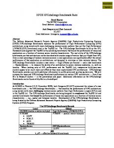
Ideal Blackscholes Bodytrack Canneal Dedup Facesim Ferret Fluidanimate Freqmine Streamcluster Swaptions Vips X264 16
Figure 1: Upper bound for speedup of PARSEC workloads with input set simlarge based on instruction count. Limitations are caused by serial sections, growing parallelization overhead and redundant computations.
X264
Vips
Ferret
Figure 2: Parallelization overhead of PARSEC benchmarks. The chart shows the slowdown of the parallel version on 1 core over the serial version.
has enough threads to occupy the whole CMP, and it is the responsibility of the scheduler to assign cores to threads in a manner that maximizes the overall throughput of the pipeline. Over time, the number of threads active for each stage will converge against the inverse throughput ratios of the individual pipeline stages relative to each other.
made measurements difficult. We do not consider this a problem because in this study we focus on trends of ratios, and quantities that small do not have a noticeable impact. It is however an issue for the analysis of working sets if the miss rate falls below this threshold and continues to decrease slowly. Only few programs are affected, and our estimate of their working set sizes might be slightly off in these cases. This is primarily an issue inherent to experimental working set analysis, since it requires well-defined points of inflection for conclusive results. Moreover, we believe that in these cases the working set size varies nondeterministically, and researchers should expect slight variations for each benchmark run.
Woo et al. use an abstract machine model with a uniform instruction latency of one cycle to measure the speedups of the SPLASH-2 programs[44]. They justify their approach by pointing out that the impact of the timing model on the characteristics which they measure - including speedup - is likely to be low. Unfortunately, this is not true in general for PARSEC workloads. While we have verified in Section 4.2 that the fundamental program properties such as miss rate and instruction count are largely not susceptible to timing shocks, the synchronization and timing behavior of the programs is. Using a timing model with perfect caches significantly alters the behavior of programs with unbounded working sets, for example how long locks to large, shared data structures are held. Moreover, any changes of the timing model have a strong impact on the number of active threads of programs which employ thread specialization. It will thus affect the load balance and synchronization behavior of these workloads. We believe it is not possible to discuss the timing behavior of these programs without also considering for example different schedulers, which is beyond the scope of this paper. Similar dependencies of commercial workloads on their environment are already known[9, 4].
The implications of these results are twofold: First, they show that our methodology is not susceptible to the nondeterministic effects of multi-threaded programs in a way that might invalidate our findings. Second, they also confirm that the metrics which we present in this paper are fundamental program properties which cannot be distorted easily. The reported application characteristics are likely to be preserved on a large range of architectures.
5.
Swaptions
12
Streamcluster
8
Number of Cores
Freqmine
4
Fluidanimate
0
0.00%
Facesim
0
2.50%
Dedup
4
5.00%
Canneal
8
7.50%
Bodytrack
12
Blackscholes
Achievable Speedup
16
PARALLELIZATION
In this section we discuss the parallelization of the PARSEC suite. As we will see in Section 6, several PARSEC benchmarks (canneal, dedup, ferret and freqmine) have working sets so large they should be considered unbounded for an analysis. These working sets are only limited by the amount of main memory in practice and they are actively used for inter-thread communication. The inability to use caches efficiently is a fundamental property of these program and affects their concurrent behavior. Furthermore, dedup and ferret use a complex, heterogeneous parallelization model in which specialized threads execute different functions with different characteristics at the same time. These programs employ a pipeline with dedicated thread pools for each parallelized pipeline stage. Each thread pool
Unlike Woo et al. who measured actual concurrency on an abstract machine, we therefore decided to analyze inherent concurrency and its limitations. Our approach is based on the number of executed instructions in parallel and serial regions of the code. We neglect any delays due to blocking on contended locks and load imbalance. This methodology is feasible because we do not study performance, our interest is in fundamental program characteristics. The presented data is largely timing-independent and a suitable measure of the concurrency inherent in a workload. The results in 15
Princeton University Technical Report TR-811-08, January 2008 Figure 1 show the maximum achievable speedup measured that way. The numbers account for limitations such as unparallelized code sections, synchronization overhead and redundant computations. PARSEC workloads can achieve actual speedups close to the presented numbers. We verified on a large range of architectures that lock contention and other timing-dependent factors are not limiting factors, but we know of no way to show it in a platform-independent way given the complications outlined above. The maximum speedup of bodytrack, x264 and streamcluster is limited by serial sections of the code. fluidanimate is primarily limited by growing parallelization overhead. On real machines, x264 is furthermore bound by a data dependency between threads, however this has only a noticeable impact on machines larger than the ones described here. It is recommended to run x264 with more threads than cores, since modeling and exposing these dependencies to the scheduler is a fundamental aspect of its parallel algorithm, comparable to the parallel algorithms of dedup and ferret. Figure 2 shows the slowdown of the parallel version on 1 core over the serial version. The numbers show that all workloads use efficient parallel algorithms which are not substantially slower than the corresponding serial algorithms.
strained input set such as simlarge, their working sets can reach hundreds of megabytes. Moreover, the need of those workloads for cache capacity is nearly insatiable and grows with the amount of data which they process. In Table 3 we give our estimates for the largest working set of each PARSEC workload for the native input set. In several cases they are significantly larger and can even reach gigabytes. These large working sets are often the consequence of an algorithm that operates on large amounts of collected input data. ferret for example keeps a data base of feature vectors of images in memory to find the images most similar to a given query image. The cache and memory needs of these applications should be considered unbounded, as they become more useful to their users if they can work with increased amounts of data. Programs with unbounded working sets are canneal, dedup, ferret and freqmine. In Figure 4 we present our analysis of the spatial locality of the PARSEC workloads. The data shows how the miss rate of a shared cache changes with line size. All programs benefit from larger cache lines, but to different extents. facesim, fluidanimate and streamcluster show the greatest improvement as the line size is increased, up to the the maximum value of 256 bytes which we used. These programs have streaming behavior, and an increased line size has a prefetching effect which these workloads can take advantage of. facesim for example spends most of its time updating the position-based state of the model, for which it employs an iterative Newton-Raphson algorithm. The algorithm iterates over the elements of a sparse matrix which is stored in two one-dimensional arrays, resulting in a streaming behavior. All other programs also show good improvement of the miss rate with larger cache lines, but only up to line sizes of about 128 bytes. The miss rate is not substantially reduced with larger lines. This is due to a limited size of the basic data structures employed by the programs. They represent independent logical units, each of which is intensely worked with during a computational phase. For example, x264 operates on macroblocks of 8 × 8 pixels at a time, which limits the sizes of the used data structures. Processing a macroblock is computationally intensive and largely independent from other macroblocks. Consequently, the amount of spatial locality is bounded in these cases.
PARSEC programs scale well enough to study CMPs. We believe they are also useful on machines larger than the ones analyzed here. The PARSEC suite exhibits a wider variety of parallelization models than previous benchmark suites such as the pipeline model. Some of its workloads can adapt to different timing models and can use threads to hide latencies. It is important to analyze these programs in the context of the whole system.
6.
WORKING SETS AND LOCALITY
The temporal locality of a program can be estimated by analyzing how the miss rate of a processor’s cache changes as its capacity is varied. Often the miss rate does not decrease continuously as the size of a cache is increased, but stays on a certain level and then makes a sudden jump to a lower level when the capacity becomes large enough to hold the next important data structure. For CMPs an efficient functioning of the last cache level on the chip is crucial because a miss in the last level will require an access to off-chip memory.
For the rest of our analysis we chose a cache capacity of 4 MB for all experiments. We could have used a matching cache size for each workload, but that would have made comparisons very difficult, and the use of very small or very large cache sizes is not realistic. Moreover, in the case of the workloads with an unbounded working set size, a working set which completely fits into a cache would be an artifact of the limited simulation input size and would not reflect realistic program behavior.
To analyze the working sets of the PARSEC workloads we studied a cache shared by all processors. Our results are presented in Figure 3. In Table 3 we summarize the important characteristics of the identified working sets. Most workloads exhibit well-defined working sets with clearly identifiable points of inflection. Compared to SPLASH-2, PARSEC working sets are significantly larger and can reach hundreds of megabytes such as in the cases of canneal and freqmine. Two types of workloads can be distinguished: The first group contains benchmarks such as bodytrack and swaptions which have working sets no larger than 16 MB. These workloads have a limited need for caches with a bigger capacity, and the latest generation of CMPs often already has caches sufficiently large to accommodate most of their working sets. The second group of workloads is composed of the benchmarks canneal, ferret, facesim, fluidanimate and freqmine. These programs have very large working sets of sizes 65 MB and more, and even with a relatively con-
7.
COMMUNICATION-TO-COMPUTATION RATIO AND SHARING
In this section we discuss how PARSEC workloads use caches to communicate. Most PARSEC benchmarks share data intensely. Two degrees of sharing can be distinguished: Shared data can be read-only during the parallel phase, in which case it is only used for lookups and analysis. Input data is frequently used in such a way. But shared data can also be used for communication between threads, in which 16
Princeton University Technical Report TR-811-08, January 2008 blackscholes
15.00%
WS1
1.50%
WS2
WS1
WS2
1.00%
10.00%
WS1
1.50%
WS2
WS2
1.00%
10.00%
0.50%
0.50%
ferret
WS2
WS1
6.00%
1.50% 2.00%
WS2
WS1
1.00% 2.00%
0.00%
0.00%
WS2
5.00%
1 2 4 8 16 32 64 128 256 512 1024 2048 4096 8192 16384 32768 65536 131072 262144
0.00%
Cache Size (KB)
x264
vips
5.00%
10.00%
10.00%
4.00%
8.00%
8.00%
3.00%
6.00%
2.00%
WS1
4.00%
WS1
WS2
WS2
4.00%
2.00%
2.00%
0.00%
0.00%
0.00%
Cache Size (KB)
WS1
6.00%
1.00%
1 2 4 8 16 32 64 128 256 512 1024 2048 4096 8192 16384 32768 65536 131072 262144
10.00%
1 2 4 8 16 32 64 128 256 512 1024 2048 4096 8192 16384 32768 65536 131072 262144
1 2 4 8 16 32 64 128 256 512 1024 2048 4096 8192 16384 32768 65536 131072 262144
WS1
0.00%
0.00%
swaptions
streamcluster 20.00%
15.00%
0.50%
1 2 4 8 16 32 64 128 256 512 1024 2048 4096 8192 16384 32768 65536 131072 262144
1.00%
WS2
WS2
4.00%
2.00%
WS1
1.00%
1 2 4 8 16 32 64 128 256 512 1024 2048 4096 8192 16384 32768 65536 131072 262144
3.00%
8.00%
2.00%
3.00%
1 2 4 8 16 32 64 128 256 512 1024 2048 4096 8192 16384 32768 65536 131072 262144
WS1
freqmine
fluidanimate
10.00%
4.00%
1 2 4 8 16 32 64 128 256 512 1024 2048 4096 8192 16384 32768 65536 131072 262144
1 2 4 8 16 32 64 128 256 512 1024 2048 4096 8192 16384 32768 65536 131072 262144
1 2 4 8 16 32 64 128 256 512 1024 2048 4096 8192 16384 32768 65536 131072 262144
facesim 5.00%
0.00%
0.00%
0.00%
1 2 4 8 16 32 64 128 256 512 1024 2048 4096 8192 16384 32768 65536 131072 262144
0.00%
Miss Rate (%)
20.00%
2.00%
1 2 4 8 16 32 64 128 256 512 1024 2048 4096 8192 16384 32768 65536 131072 262144
Miss Rate (%)
WS1
20.00%
dedup
30.00%
2.00%
5.00%
Miss Rate (%)
canneal
bodytrack
25.00%
Cache Size (KB)
Cache Size (KB)
Figure 3: Miss rates versus cache size. Data assumes a shared 4-way associative cache with 64 byte lines. WS1 and WS2 refer to important working sets which we analyze in more detail in Table 3. Cache requirements of PARSEC benchmark programs can reach hundreds of megabytes.
Program
blackscholes bodytrack canneal dedup facesim ferret fluidanimate freqmine streamcluster swaptions vips x264
Input Set simlarge Working Set 1 Data Size Growth Structure(s) Rate options 64 KB C edge maps 512 KB const. elements 64 KB C data chunks 2 MB C tetrahedra 256 KB C images 128 KB C cells 128 KB C transactions 256 KB C data points 64 KB C swaptions 512 KB C image data 64 KB C macroblocks 128 KB C
Working Set 2 Data Size Growth Structure(s) Rate portfolio data 2 MB C input frames 8 MB const. netlist 256 MB DS hash table 256 MB DS face mesh 256 MB DS data base 64 MB DS particle data 64 MB DS FP-tree 128 MB DS data block 16 MB user-def. same as WS1 same same image data 16 MB C reference frames 16 MB C
Input Set native Working Set 2 Size Estimate same same 2 GB 2 GB same 128 MB 128 MB 1 GB 256 MB same same same
Table 3: Important working sets and their growth rates. DS represents the data set size and C is the number of cores. Working set sizes are taken from Figure 3. Values for native input set are analytically derived estimates. Working sets that grow proportional to the number of cores C are aggregated private working sets and can be split up to fit into correspondingly smaller, private caches.
17
Princeton University Technical Report TR-811-08, January 2008 15.00%
1.00%
Miss Rate (%)
0.75% 10.00%
Stores
0.50%
Loads 5.00%
0.25%
0.00%
blackscholes fluidanimate swaptions bodytrack freqmine
canneal
dedup
facesim
ferret
streamcluster
vips
8 16 32 64 128 256
8 16 32 64 128 256
8 16 32 64 128 256
8 16 32 64 128 256
8 16 32 64 128 256
8 16 32 64 128 256
8 16 32 64 128 256
8 16 32 64 128 256
8 16 32 64 128 256
8 16 32 64 128 256
8 16 32 64 128 256
8 16 32 64 128 256
0.00%
x264
Figure 4: Miss rates as a function of line size. Data assumes 8 cores sharing a 4-way associative cache with 4 MB capacity. Miss rates are broken down to show the effect of loads and stores. 55.00% 50.00%
Shared Lines (%)
45.00% 40.00% 35.00%
>8 Sharers 8 Sharers
30.00%
7 Sharers
25.00%
6 Sharers
20.00%
5 Sharers 4 Sharers
15.00%
3 Sharers 2 Sharers
10.00% 5.00%
bodytrack blackscholes
dedup
ferret
freqmine
swaptions
vips
8 16 32 64 128 256
8 16 32 64 128 256
8 16 32 64 128 256
8 16 32 64 128 256
8 16 32 64 128 256
8 16 32 64 128 256
8 16 32 64 128 256
8 16 32 64 128 256
0.00%
x264
Figure 5: Portion of a 4-way associative cache with 4 MB capacity which is shared. The line size is varied from 8 to 256 bytes. Data assumes 8 cores and is broken down to show the number of threads sharing the lines. case it is also modified during the parallel phase. In Figure 5 we show how the line size affects sharing. The data combines the effects of false sharing and the access pattern of the program due to constrained cache capacity. In Figure 6, we analyze how the program uses its data. The chart shows what data is accessed and how intensely it is used. The information is broken down in two orthogonal ways, resulting in four possible types of accesses: Read and write accesses and accesses to thread-private and shared data. Additionally, we give numbers for true shared accesses. An access is a true access if the last reference to that line came from another thread. True sharing does not count repeated accesses by the same thread. It is a useful metric to estimate the requirements for the cache coherence mechanism of a CMP: A true shared write can trigger a coherence invalidate or update, and a true shared read might require the replication of data. All programs exhibit very few true shared writes. Cache misses are not included in Figure 6, we analyze them
separately when we discuss off-chip traffic in Section 8. Four programs (canneal, facesim, fluidanimate and streamcluster) showed only trivial amounts of sharing. They have therefore not been included in Figure 5. In the case of canneal, this is a results of the small cache capacity. Most of its large working set is shared and actively worked with by all threads. However, only a minuscule fraction of it fits into the cache, and the probability that a line is accessed by more than one thread before it gets replaced is very small in practice. With a 256 MB cache, 58% of its cached data is shared. blackscholes shows a substantial amount of sharing, but almost all its shared data is only accessed by two threads. This is a side-effect of the parallelization model: At the beginning of the program, the boss threads initializes the portfolio data before it spawns worker threads which process parts of it in a data-parallel way. As such, the entire portfolio is shared between the boss thread and its workers, but
18
Princeton University Technical Report TR-811-08, January 2008 5
Traffic (Bytes / Instr.)
4
True Shared Writes True Shared Reads
3
Shared Writes 2
Shared Reads
1
Private Reads
Private Writes
dedup
facesim
ferret
streamcluster fluidanimate freqmine swaptions
1 2 4 8 16
1 2 4 8 16
1 2 4 8 16
1 2 4 8 16
1 2 4 8 16
1 2 4 8 16
1 2 4 8 16
1 2 4 8 16
canneal
1 2 4 8 16
1 2 4 8 16
blackscholes bodytrack
1 2 4 8 16
1 2 4 8 16
0
vips x264
Figure 6: Traffic from cache in bytes per instruction for 1 to 16 cores. Data assumes a shared 4-way associative cache with 64 byte lines. Results are broken down in accesses to private and shared data. True accesses do not count repeated accesses from the same thread. the worker threads can process the options independently from each other and do not have to communicate with each other. ferret shows a modest amount of data sharing. Like the sharing behavior of canneal, this is caused by severely constrained cache capacity. ferret uses a database that is scanned by all threads to find entries similar to the query image. However, the size of the database is practically unbounded, and because threads do not coordinate their scans with each other it is unlikely that a cache line gets accessed more than once. bodytrack and freqmine exhibit substantial amounts of sharing due to the fact that threads process the same data. The strong increase of sharing of freqmine is caused by false sharing, as the program uses an arraybased tree as its main data structure. Larger cache lines will contain more nodes, increasing the chance that the line is accessed by multiple threads. vips has some shared data which is mostly used by only two threads. This is also predominantly an effect of false sharing since image data is stored in a consecutive array which is processed in a dataparallel way by threads. x264 uses significant amounts of shared data, most of which is only accessed by a low number of threads. This data is the reference frames, since a thread needs this information from other stages in order to encode the frame it was assigned. Similarly, the large amount of shared data of dedup is the input which is passed from stage to stage.
for inter-thread communication. As WS1 grows, it starts to displace WS2, and the threads are forced to communicate via main memory. Two more programs which communicate intensely are dedup and ferret. Both programs use the pipeline parallelization model with dedicated thread pools for each parallel stage, and all data has to be passed from stage to stage. fluidanimate also shows a large amount of inter-thread communication, and its communication needs grow as the number of threads increase. This is caused by the spatial partitioning that fluidanimate uses to distribute the work to threads. Smaller partitions mean a worse surface to volume ratio, and communication grows with the surface. Overall, most PARSEC workloads have complex sharing patterns and communicate actively. Pipelined programs can require a large amount of bandwidth between cores in order to communicate efficiently. Shared caches with insufficient capacity can limit the communication efficiency of workloads, since shared data structures might get displaced to memory.
8.
OFF-CHIP TRAFFIC
In this section we analyze what the off-chip bandwidth requirements of PARSEC workloads are. Our goal is to understand how the traffic of an application grows as the number of cores of a CMP increases and how the memory wall will limit performance. We again simulated a shared cache and analyze how traffic develops as the number of cores increases. Our results are presented in Figure 7.
Most PARSEC workloads use a significant amount of communication, and in many cases the volume of traffic between threads can be so high that efficient data exchange via a shared cache is severely constrained by its capacity. An example for this is x264. Figure 6 shows a large amount of writes to shared data, but contrary to intuition its share diminishes rapidly as the number of cores is increased. This effect is caused by a growth of the working sets of x264: Table3 shows that both working set WS1 and WS2 grow proportional to the number of cores. WS1 is mostly composed of thread-private data and is the one which is used more intensely. WS2 contains the reference frames and is used
The data shows that the off-chip bandwidth requirements of blackscholes are small enough so that memory bandwidth is unlikely to be an issue. bodytrack, dedup, fluidanimate, freqmine, swaptions and x264 are more demanding. Moreover, these programs exhibit a growing bandwidth demand per instruction as the number of cores increases. In the case of bodytrack, most off-chip traffic happens in short, intense bursts since the off-chip communication predominantly 19
0.1
1
0.08
0.75
0.05
0.5
Writebacks Stores
dedup blackscholes freqmine bodytrack swaptions fluidanimate
facesim
x264 canneal
1 2 4 8 16
1 2 4 8 16
1 2 4 8 16
1 2 4 8 16
1 2 4 8 16
1 2 4 8 16
1 2 4 8 16
0
1 2 4 8 16
0 1 2 4 8 16
0.25
1 2 4 8 16
0.03
1 2 4 8 16
Loads
1 2 4 8 16
Traffic (Bytes/Instr.)
Princeton University Technical Report TR-811-08, January 2008
streamcluster ferret
vips
Figure 7: Breakdown of off-chip traffic into bytes for loads, stores and write-backs per instructions. Results are shown for 1 to 16 cores. Data assumes a 4-way associative 4 MB cache with 64 byte lines, allocate-on-store and write-back policy. takes place during the edge map computation. This phase is only a small part of the serial runtime, but on machines with constrained memory bandwidth it quickly becomes the limiting factor for scalability. The last group of programs is composed of canneal, facesim, ferret, streamcluster and vips. These programs have very high bandwidth requirements and also large working sets. canneal shows a decreasing demand for data per instruction with more cores. This behavior is caused by improved data sharing.
prepared for the demands of future applications. Many architectural problems still have to be solved to create microprocessors which are ready for the next generation of workloads. Large working sets and high off-chip bandwidth demands might limit the scalability of future programs. PARSEC can be used to drive research efforts by application demands.
10.
It is important to point out that these numbers do not take the increasing instruction throughput of a CMP into account as its number of cores grows. A constant traffic amount in Figure 7 means that the bandwidth requirements of an application which scales linearly will grow exponentially. Since many PARSEC workloads have high bandwidth requirements and working sets which exceed conventional caches by far, off-chip bandwidth will be their most severe limitation of performance. Substantial architectural improvements are necessary to allow emerging workloads to take full advantage of larger CMPs.
9.
ACKNOWLEDGMENTS
First and foremost we would like to acknowledge the many authors of the PARSEC benchmark programs which are too numerous to be listed here. The institutions who contributed the most number of programs are Intel and Princeton University. Stanford University allowed us to use their code and data for facesim. We would like to acknowledge the contribution of the following individuals: Justin Rattner, Pradeep Dubey, Tim Mattson, Jim Hurley, Bob Liang, Horst Haussecker, Yemin Zhang, and Ron Fedkiw. They convinced skeptics and supported us so that a project the size of PARSEC could succeed.
CONCLUSIONS
11.
The PARSEC benchmark suite is designed to provide parallel programs for the study for CMPs. It focuses on emerging desktop and server applications and does not have the limitations of other benchmark suites. It is diverse enough to be considered representative, it is not skewed towards HPC programs, it uses state-of-art algorithms and it supports research. In this study we characterized the PARSEC workloads to provide the basic understanding necessary to allow other researchers the effective use of PARSEC for their studies. We analyzed the parallelization, the working sets and locality, the communication-to-computation ratio and the off-chip traffic of its workloads. The high cost of microarchitectural simulation forced us to use smaller machine and problem sizes than we would really like to evaluate.
REFERENCES
[1] MediaBench II. http://euler.slu.edu/~fritts/mediabench/. [2] Pin. http://rogue.colorado.edu/pin/. [3] Elephants Dream. http://www.elephantsdream.org/, 2006. [4] A. Alameldeen, C. Mauer, M. Xu, P. Harper, M. Martin, and D. Sorin. Evaluating Non-Deterministic Multi-Threaded Commercial Workloads. In Proceedings of the Computer Architecture Evaluation using Commercial Workloads, February 2002. [5] A. Alameldeen and D. Wood. Variability in Architectural Simulations of Multi-threaded Workloads. In Proceedings of the 9th International Symposium on High-Performance Computer Architecture, February 2003. [6] A. Balan, L. Sigal, and M. Black. A Quantitative Evaluation of Video-based 3D Person Tracking. In IEEE Workshop on VS-PETS, pages 349–356, 2005.
Our analysis shows that current CMPs are not sufficiently 20
Princeton University Technical Report TR-811-08, January 2008
[7] P. Banerjee. Parallel algorithms for VLSI computer-aided design. Prentice-Hall, Inc., Upper Saddle River, NJ, USA, 1994.
[25] M.-L. Li, R. Sasanka, S. V. Adve, Y.-K. Chen, and E. Debes. The ALPBench Benchmark Suite for Complex Multimedia Applications. In Proceedings of the 2005 International Symposium on Workload Characterization, October 2005. [26] C. Lucchese, S. Orlando, R. Perego, and F. Silvestri. WebDocs: a real-life huge transactional dataset. In 2nd IEEE ICDM Workshop on Frequent Itemset Mining Implementations 2004, November 2004. [27] Q. Lv, W. Josephson, Z. Wang, M. Charikar, and K. Li. Ferret: A Toolkit for Content-Based Similarity Search of Feature-Rich Data. In Proceedings of the 2006 EuroSys Conference, pages 317–330, 2006. [28] Q. Lv, W. Josephson, Z. Wang, M. Charikar, and K. Li. Multi-Probe LSH: Efficient Indexing for High-Dimensional Similarity Search. In Proceedings of the 33rd International Conference on Very Large Data Bases, pages 950–961, 2007. [29] U. Manber. Finding Similar Files in a Large File System. In Proceedings of the USENIX Winter 1994 Technical Conference, pages 1–10, San Fransisco, CA, USA, October 1994. [30] K. Martinez and J. Cupitt. VIPS - a highly tuned image processing software architecture. In Proceedings of the 2005 International Conference on Image Processing, volume 2, pages 574–577, September 2005. [31] M. Matsumoto and T. Nishimura. Mersenne Twister: A 623-dimensionally equidistributed uniform pseudorandom number generator. In ACM Transactions on Modeling and Computer Simulation, volume 8, pages 3–30, January 1998. [32] M. M¨ uller, D. Charypar, and M. Gross. Particle-Based Fluid Simulation for Interactive Applications. In Proceedings of the 2003 ACM SIGGRAPH/Eurographics Symposium on Computer Animation, pages 154–159, Aire-la-Ville, Switzerland, Switzerland, 2003. Eurographics Association. [33] R. Nock and F. Nielsen. Statistical Region Merging. IEEE Transactions on Pattern Analysis and Machine Intelligence, 26:1452–1458, 2004. [34] L. O’Callaghan, A. Meyerson, R. M. N. Mishra, and S. Guha. High-Performance Clustering of Streams and Large Data Sets. In Proceedings of the 18th International Conference on Data Engineering, February 2002. [35] D. Pnueli and C. Gutfinger. Fluid Mechanics. Cambridge University Press, 1992. [36] S. Quinlan and S. D. Venti. A New Approach to Archival Storage. In Proceedings of the USENIX Conference on File And Storage Technologies, January 2002. [37] Y. Rubner, C. Tomasi, and L. J. Guibas. The Earth Mover’s Distance as a Metric for Image Retrieval. International Journal of Computer Vision, 40:99–121, 2000. [38] E. Sifakis, I. Neverov, and R. Fedkiw. Automatic Determination of Facial Muscle Activations from Sparse Motion Capture Marker Data. ACM Transactions on Graphics, 24(3):417–425, 2005. [39] N. T. Spring and D. Wetherall. A Protocol-Independent Technique for Eliminating Redundant Network Traffic. In Proceedings of ACM SIGCOMM, August 2000. [40] J. Teran, E. Sifakis, G. Irving, and R. Fedkiw. Robust Quasistatic Finite Elements and Flesh Simulation. In Proceedings of the 2005 ACM SIGGRAPH/Eurographics Symposium on Computer Animation, pages 181–190, New York, NY, USA, 2005. ACM Press. [41] D. Vatolin, D. Kulikov, and A. Parshin. MPEG-4 AVC/H.264 Video Codecs Comparison. http://compression.ru/video/codec_comparison/pdf/ msu_mpeg_4_avc_h264_co%dec_comparison_2007_eng.pdf, 2007.
[8] J. Barnes and P. Hut. A hierarchical O(N log N) force-calculation algorithm. Nature, 324:446–449, December 1986. [9] L. Barroso, K. Gharachorloo, and F. Bugnion. Memory System Characterization of Commercial Workloads. In Proceedings of the 25th International Symposium on Computer Architecture, pages 3–14, June 1998. [10] Black, Fischer, and Scholes. The Pricing of Options and Corporate Liabilities. Journal of Political Economy, 81:637–659, 1973. [11] S. Brin, J. Davis, and H. Garcia-Molina. Copy Detection Mechanisms for Digital Documents. In Proceedings of Special Interest Group on Management of Data, 1995. [12] M. Desbrun and M.-P. Gascuel. Smoothed Particles: A new paradigm for animating highly deformable bodies. In Computer Animation and Simulation ’96, pages 61–76, August 1996. [13] J. Deutscher and I. Reid. Articulated Body Motion Capture by Stochastic Search. International Journal of Computer Vision, 61(2):185–205, February 2005. [14] P. Dubey. Recognition, Mining and Synthesis Moves Computers to the Era of Tera. Technology@Intel Magazine, February 2005. [15] G. Grahne and J. Zhu. Efficiently Using Prefix-trees in Mining Frequent Itemsets. November 2003. [16] J. Han, J. Pei, and Y. Yin. Mining Frequent Patterns without Candidate Generation. In W. Chen, J. Naughton, and P. A. Bernstein, editors, 2000 ACM SIGMOD International Conference on Management of Data, pages 1–12. ACM Press, 05 2000. [17] D. Heath, R. Jarrow, and A. Morton. Bond Pricing and the Term Structure of Interest Rates: A New Methodology for Contingent Claims Valuation. Econometrica, 60(1):77–105, January 1992. [18] J. L. Hennessy and D. A. Patterson. Computer Architecture: A Quantitative Approach. Morgan Kaufmann, 2003. [19] L. Hernquist and N. Katz. TreeSPH - A unification of SPH with the hierarchical tree method. The Astrophysical Journal Supplement Series, 70:419, 1989. [20] C. J. Hughes, R. Grzeszczuk, E. Sifakis, D. Kim, S. Kumar, A. P. Selle, J. Chhugani, M. Holliman, and Y.-K. Chen. Physical Simulation for Animation and Visual Effects: Parallelization and Characterization for Chip Multiprocessors. SIGARCH Computer Architecture News, 35(2):220–231, 2007. [21] J. C. Hull. Options, Futures, and Other Derivatives. Prentice Hall, 2005. [22] A. Jaleel, M. Mattina, and B. Jacob. Last-Level Cache (LLC) Performance of Data-Mining Workloads on a CMP A Case Study of Parallel Bioinformatics Workloads. In Proceedings of the 12th International Symposium on High Performance Computer Architecture, February 2006. [23] Jayaprakash Pisharath and Ying Liu and Wei-keng Liao and Alok Choudhary and Gokhan Memik and Janaki Parhi. NU-Minebench 2.0. Technical report, Center for Ultra-Scale Computing and Information Security Northwestern University, August 2005. [24] R. M. Karp and M. O. Rabin. Efficient Randomized Pattern-Matching Algorithms. IBM Journal of Research and Development, 31(2):249–260, 1987.
21
Princeton University Technical Report TR-811-08, January 2008 [42] L. Verlet. Computer Experiments on Classical Fluids. I. Thermodynamical Properties of Lennard-Jones Molecules. Physical Review, 159:98–103, 1967. [43] T. Wiegand, G. J. Sullivan, G. Bjontegaard, and A. Luthra. Overview of the H.264/AVC Video Coding Standard. IEEE Transactions on Circuits and Systems for Video Technology, 13(7):560–576, 2003. [44] S. C. Woo, M. Ohara, E. Torrie, J. P. Singh, and A. Gupta. The SPLASH-2 Programs: Characterization and Methodological Considerations. In Proceedings of the 22nd International Symposium on Computer Architecture, pages 24–36, June 1995. [45] G. Xu. A New Parallel N-Body Gravity Solver: TPM. The Astrophysical Journal Supplement Series, 98:355, 1995. [46] T. Y. Yeh, P. Faloutsos, S. Patel, and G. Reinman. ParallAX: An Architecture for Real-Time Physics. In Proceedings of the 34th International Symposium on Computer Architecture, June 2007.
22