The Phase Diagram of 1-in-3 Satisfiability Problem

The Phase Diagram of 1-in-3 Satisfiability Problem 1

Jack Raymond1 , Andrea Sportiello2 , Lenka Zdeborov´a3

NCRG; Aston University, Aston Triangle, Birmingham, B4 7EJ Universit` a degli Studi di Milano, via Celoria 16, I-20133 Milano CNRS; Univ. Paris-Sud, UMR 8626, Orsay CEDEX, France 91405, LPTMS (Dated: February 6, 2008)

arXiv:cond-mat/0702610v2 [cond-mat.stat-mech] 11 Apr 2007

2

3

We study the typical case properties of the 1-in-3 satisfiability problem, the boolean satisfaction problem where a clause is satisfied by exactly one literal, in an enlarged random ensemble parametrized by average connectivity and probability of negation of a variable in a clause. Random 1-in-3 Satisfiability and Exact 3-Cover are special cases of this ensemble. We interpolate between these cases from a region where satisfiability can be typically decided for all connectivities in polynomial time to a region where deciding satisfiability is hard, in some interval of connectivities. We derive several rigorous results in the first region, and develop the one-step–replica-symmetrybreaking cavity analysis in the second one. We discuss the prediction for the transition between the almost surely satisfiable and the almost surely unsatisfiable phase, and other structural properties of the phase diagram, in light of cavity method results. PACS numbers: 89.20.Ff, 75.10.Nr, 05.70.Fh, 02.70.-r

I.

INTRODUCTION AND MOTIVATION

Classification of the average-case computational complexity of the constraint satisfaction problems is a major task in theoretical computer science. Many problems were successfully analyzed by rigorous probabilistic methods. However, the average-case complexity remains an open question for most of the well known NP-complete problems [1, 2], for example the K-satisfiability, Vertex Coloring, and also 1in-K satisfiability, on the commonly studied random ensembles (sparse random regular or Erd¨ os-R´enyi graphs). In recent years heuristic methods from statistical physics [3, 4, 5] have allowed us to understand some average-case properties of large random instances [6]. The aim of these studies was not to prove average NP-completeness [7], it was rather to understand why the problems appear hard for some local algorithms, in some intervals of ensemble parametrization. These efforts culminated in designing a new polynomial algorithm, survey propagation [8, 9], which empirically outspeeds all the previously known heuristics. Rigorous undertanding of this algorithm is, however, still missing. The fact that lies behind this success is the intrinsic similarity of the combinatorial optimization problems to physical systems called spin glasses [10]. The organization of solutions is analogous to the structure of the free energy landspace of the physical models. Several phases can be located in the parameter space, with abrupt transitions between the different phases. An example is the SAT/UNSAT transition, i.e. the transition from the SATisfiable (SAT) phase where almost every instance is satisfiable (ground state of energy zero) to the UNSATisfiable (UNSAT) phase where almost every instance is unsatisfiable (positive ground-state energy). Another is the glassy transition where the phase space splits into many clusters and metastable states, and where many dynamical procedures (a physical dynamics or an algorithm) are unable to find the ground state. This connection between the structure of solution and the average algorithmic performance was the main motivation for detailed studies of the phase diagram of the K-satisfiability [5, 8, 9, 11], Vertex Coloring [12, 13] and many other problems. The presented study of the phase diagram of the 1-in-K satisfiability (sometimes called exact satisfiability [14]) problem adds one more item to this list. But prolonging a list is not the main motivation for this work. 1-in-K SAT on the symmetric ensemble (probability that a variable in a clause is negated is 1/2) is one of the few NP-complete problem which has been proven to be on average polynomial (Easy) [15]. On the other hand for the positive ensemble (no negations, equivalent to Exact Cover) no such proof exists, nor is there a heuristic algorithm with empirically polynomial time performance in the vinicity of the SAT/UNSAT transition. However, by analogy with K-SAT and coloring, we may expect polynomial time performance in this region using survey propagation. Our main motivation is to interpolate between the symmetric and positive ensemble to show how the phase space changes. For this reason we introduce a ǫ–1-in-K SAT problem, and study the phase diagram in parameters (γ, ǫ), where ǫ stays for the probability that a variable in a clause is negated, and γ is the average connectivity of a variable. To our knowledge, this general ensemble is considered here for the first time. We generalize the rigorous probabilistic analysis to the general ǫ case. Then we use the replica-

2 symmetric and one-step–replica-symmetry-breaking cavity methods [3, 4] to understand more features of the problem in the whole space of parameters. Our motivation is similar to the one which led to the introduction of the (2+p)-SAT problem [16, 17, 18], where the instances are a mixture of 2-SAT and 3-SAT clauses on Erd¨ os-R´enyi graphs. A parameter p interpolates between the ensemble of random 3-SAT formulas, which are know to be computationally hard [8, 9] in a region including the SAT/UNSAT transition, and random 2-SAT formulas, for which an anycase polynomial algorithm exists. A statistical physics approach has been applied to study the (2 + p)-SAT problem, however only the replica-symmetric solution was investigated. Analogical interpolation between P and NP-complete cases of some other problems have been investigated in [19, 20]. A.

The model

A factor graph G = (Vv , Vc ; E) is a bipartite graph, where the two species of vertices are called respectively variables i ∈ Vv and clauses a ∈ Vc . It is a common graphical object used in computer science in order to encode the geometrical framework of a problem in combinatorial optimization, as it often allows us to shorten and clarify the “rules of the game”. This is the case also for 1-in-K-SAT. Indeed, cases of both K-SAT and 1-in-K-SAT are example of boolean satisfiability problems, and thus formally inscribed in a framework of boolean logic expressions: we deal with M boolean clauses over N variables, which should be simultaneously satisfied (i.e. evalued to True), in order to consider the N -tuple of assignments to the variables a solution of the problem instance. Each clause a involves K out of the 2N literals x1 , . . . , xN , x ¯1 , . . . , x ¯N (not xi and x¯i simultaneously). While a K-SAT clause is satisfied if at least one of the involved literals is True, a 1-in-K-SAT clause is satisfied if exactly one of the involved literals is True. For both problems, a factor graph G (whose clause-nodes a have degree K) and a function J : E(G) → ±1 fully encode an instance: if clause a involves literal xi or x ¯i we will have an edge (i, a) ∈ E(G), and Jai = +1 or −1 respectively. It is customary to draw edges with J = +1 as solid lines, and edges with J = −1 as dashed lines. If we use the common identification with “spin variables” si xi = True xi = False

←→ ←→

si = +1 si = −1

the function E{Ja } (s) corresponding to a 1-in-K-SAT clause is ( True si1 Jai1 + · · · + siK JaiK = 2 − K E{Ja } (s) = False otherwise

(1)

V and we say that s is a solution of the given instance if a E{Ja } (s) = True. 1-in-K-SAT is polynomial in the case K = 2 (coinciding with 2-XOR-SAT, or 2-Coloring), while it is NP-complete for K ≥ 3, even in the restriction to all J’s positive (unlike K-SAT). For what concerns average-case complexity, two Erd¨ os-R´enyi-like random ensembles of instances are commonly considered. In both cases we have N variables and every possible clause is present with probability p such that the average number of clauses is M = N γ/K, and variables have Poissonian degree with average γ. Then we distinguish Positive Poisson ensemble: The edge parameters Jai are all +1. In this case we use a shorthand for the energy function EJa =(+,+,+) = Ea . Symmetric Poisson ensemble: The edge parameters Jai are random independent in {±1} with equal probability. The positive version of the problem is the one which corresponds to Exact Cover, in the case of incidence matrices whose columns have K nonzero entries. In this paper we study the generalization to the ensemble in which the J’s are taking value ±1 independently, ǫ ∈ [0, 1/2] being the probability of having J = −1. We call this generalization ǫ–1-in-K SAT, in order not to confuse with the 1-in-K SAT by which is often meant only the symmetric ensemble. We describe the phase diagram of this problem in the parameters (ǫ, γ).

3 B.

Main results and the paper organization

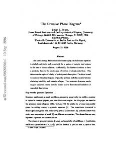
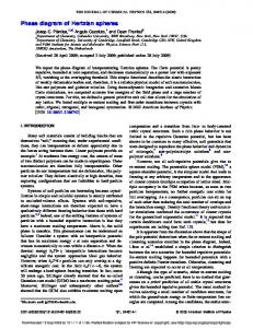
Throughout this paper we present methods and results relevant to the problem of ǫ–1-in-K-SAT with K = 3 only. Generalisation to instances of larger clause length requires, in most cases, only small changes in methodology. In section II and appendices A-B we derive algorithmic and probabilistic bounds, both rigorous, for the SAT/UNSAT threshold in the ǫ–1-in-3-SAT problem. The most remarkable result of those sections is that the bound is tight for ǫ ∈ [0.2726, 1/2], so in that interval the SAT/UNSAT threshold is rigorously known. This generalizes the result of [15] for the symmetric ensemble ǫ = 1/2. In section III we develop the Replica-Symmetric (RS) solution. First we write the replica-symmetric equations III A, then we discuss the zero-temperature limit III B. We analyze the hard-fields solution in III C, and the soft-fields solution in III D. However, as we show in III E, this solution cannot be correct (cease to be stable) above a certain connectivity not larger than the expected SAT/UNSAT transition. At this connectivity the belief propagation algorithm would fail to converge. In fact, there even exists a region in the phase diagram, where the RS solution is not stable, and yet the Short Clause Heuristics (SCH) algorithm is proven to work in on average polynomial time. To our knowledge this does not happen in any of the previously studied models, and is a point worth further investigation. In section IV we work out the one-step–Replica-Symmetry-Breaking (1RSB) solution. In this case we assume the existence of many disconnected clusters of solutions, and many metastable states, which can actually trap most of the traditional algorithms. We write the general equations in section IV A, then we concentrate on the zero-temperature zero-energy case IV B, which leads to the survey propagation equations. The zero-temperature positive-energy case is studied in appendix C. In appendix D we check the local stability of the 1RSB solution. The main result of the 1RSB analysis is the prediction for the SAT/UNSAT threshold, fig. 1. For ǫ < 0.07 the 1RSB approach is stable around the SAT/UNSAT line, so the threshold is likely to be exact. Whereas for 0.07 < ǫ < 0.2726 the 1RSB result is unstable, and a more involved analysis would be required to locate exactly the SAT/UNSAT threshold (the 1RSB result is expected to be an upper bound). The presence of a nontrivial 1RSB solution in the small-ǫ region suggests the presence of a Hard-SAT region. Details of these results are discussed in section IV C. FIG. 1: The phase diagram of ǫ–1-in-3 SAT problem, for what concerns the SAT/UNSAT transition. The parameters ǫ and γ describe the probability of negations and the average variable connectivity. For ǫ > 0.2726, ` ´ the threshold is rigorously γ ∗ (ǫ) = 1/ 4ǫ(1 − ǫ) (drawn as a solid line), since the unit-clause upper bound and short-clause-heuristic lower bound coincide in that region. For ǫ < 0.2726, the dot-dashed, dashed and dotted line denore respectively the SCH lower bound, and the UC and first-moment-method (1MM) upper bounds. The solid line is our one-step replica-symmetry-breaking (1RSB) prediction for the SAT/UNSAT threshold. For 0 ≤ ǫ < 0.07 the 1RSB result is stable (gray shading) and so the threshold is likely to be exact. For 0.07 < ǫ < 0.2726 the 1RSB result is unstable, and so the threshold is just approximate (expected to be an upper bound). γ

UC upper bound 1MM upper bound SCH lower bound 1RSB prediction stable

UNSAT

2.0 1.932 1.8789 1.8

1.639 1.6

Easy UNSAT 1.4

Easy SAT 1.2

1

1 0

0.07 0.1

0.2

0.2726 0.3

0.4

0.5

ǫ

4 II.

RIGOROUS BOUNDS ON THE SAT/UNSAT THRESHOLD A.

Unit-Clause Propagation Analysis

Unit-Clause (UC) algorithms are a class of randomized algorithms for boolean satisfiability problems, which when applied to a specific instance, seek a solution or a certificate of unsatisfiability by assigning variables to ±1 (or “True/False”) whilst maximizing the amount of logical deductions coming from uniquely determined constraints (unit clauses). In the absense of immediate deductions, variables are fixed by some heuristic rule, and these free steps determine a branching process on the space of feasible configurations. Our analysis of unit-clause propagation is elucidated in appendix A, while for a more general description consider [21]. Algorithms based on unit-clause propagation have been already analysed for the problems of symmetric and positive 1-in-K SAT. For the positive ensemble (ǫ = 0) the best known lower bound to the SAT/UNSAT transition is γ = 1.638 [22], and no upper bound is known from unit-clause algorithms. For the symmetric ensemble (ǫ = 1/2), the method allows us to determine that the exact SAT/UNSAT transition is γ = 1 [15]. Here we extend these results to compute the upper bound γuc (ǫ) and the lower bound γsch (ǫ) for general probability of negation, which describe regions that are almost surely (a.s.) Easy SAT or Easy UNSAT for an instance of the ǫ–1-in-3-SAT, sampled from the random (ǫ, γ) ensemble (cfr. section I A). In appendix A 1 we demonstrate the upper bound γuc (ǫ) to the connectivity above which an Easy UNSAT phase exists. Whenever γ > γuc (ǫ), the instance is a.s. proven to be UNSAT by a randomized linear-time decimation algorithm in which one tests, for all variables i, if both fixing si = +1 or si = −1 lead to contradictions through unit-clause implications alone. This line has the analytic form γuc (ǫ) =
1/ 4ǫ(1 − ǫ) . In appendix A 2 we obtain the lower bound γsch (ǫ) to the connectivity below which an Easy SAT phase exists. Now, we perform an extensive number of free choices, and thus we should specify our heuristic rule. It turns out that, among those tested, the Short Clause Heuristics (SCH; assigning a variable in one of the shortest clauses remaining) is the one attaing the best bound on the whole interval of ǫ. If γ < γsch (ǫ), by fixing variables according to SCH one can find a solution with finite probability on any run. Restarting the procedure many times allows us to find a solution in on average linear time. This extends the idea employed for Exact Cover in [22]. At all ǫ we find lower bounds by numerical integration (see above figure), including γsch (0) = 1.639, consistent with the analysis of [22]. Finally in appendix A 3 we prove analytically that on the interval ǫ ∈ [0.2726, 1/2] the curves γuc (ǫ) and γsch (ǫ) coincide. The result includes the symmetric ensemble, for which it was originally proven in [15]. This fact indicates that there exists a region of the phase diagram in which typical instances of the (ǫ, γ) ensemble are easily solved, except at the exactly determined SAT/UNSAT transition line. B.

Upper bounds for small ǫ

For ǫ → 0 we have γuc ∼ ǫ−1 and so we would like to find a better upper bound by some different method. An improvement is obtained through the First Moment Method (1MM) on the 2-core of the graph. Restriction to the 2-core makes the bound tighter, as it reduces instance-to-instance fluctuations. This provides a line γ1mm (ǫ), which is finite everywhere, and thus beats γuc in some interval of small ǫ (details are in appendix B 1). The best known upper bound for the positive ensemble (ǫ = 0) is γ = 1.932, obtained by a refinement of the first moment method [23]. Still, the first moment method is only probabilistic, and does not allow us to find a certificate in polynomial time for a given instance. Such a task is achieved at finite γ, also in the region of small ǫ and ǫ = 0, through the embedding of 1-in-3-SAT into an instance of 3-XOR-SAT. While Ea1-in-3 (s1 , s2 , s3 ) = True on the three configurations (s1 , s2 , s3 ) = (+, −, −), (−, +, −) and (−, −, +), the function Ea3-XOR (s1 , s2 , s3 ) also allows for (s1 , s2 , s3 ) = (+, +, +). So all the constraints are linear relations, and the problem is formally solved by Gaussian elimination. This gives an upper bound for an “Easy-UNSAT” phase, independently of ǫ at γ = 3α∗ = 2.754 where α∗ is the SAT/UNSAT threshold (clause-to-variable ratio) in 3-XOR-SAT [24, 25] (cfr. appendix B 2 for details). Note for comparison that in random 3-SAT at given finite α (however large) in the UNSAT phase, there is no polynomial algorithm which can find a.s. a certificate for a typical instance, and intuition strongly suggests that such an algorithm can not exist [26].

5 III.

RS CAVITY APPROACH

The cavity method is developed within a statistical mechanics formulation. For this purpose we choose an integer-valued “energy function” for a single clause, E{Ja } (s), to be associated to the original booleanbool bool valued function E{J (s) in (1); just as E{Ja } (s) = 0 or 1 respectively if E{J (s) = True or False. We a} a} thus have a Hamiltonian X H(s) = 2E{Ja } (s) , (2) a

which counts (twice) the number of contradictions. The factor 2 is a useful convention, so that all the cavity parameters to be introduced below (cavity fields and biases) will be integer in the “zero-temperature” limit. The introduction of the cost function above allows us to define a Gibbs weight e−βH(s) , where β is some parameter (inverse temperature), so that a single contradiction causes a dump of a factor e−2β in the measure of the configuration. As customary in statistical mechanics, one introduces a partition function X Z(β) = e−βH(s) (3) s

and a set of observables (say, probabilities of having patterns A) X prob(A) := Z −1 e−βH(s) .

(4)

s: A happens

Within this framework the cavity method translates certain obvious recurrence relations for interaction structures on a factorized graph (tree) to approximate self-consistent equations for local expectation values on a graph which is only “locally tree-like” (e.g. a sparse Erd¨ os-R´enyi graph at large N , where loops are expected to arise at lengths of order ln N ). The replica-symmetric (RS) assumption is used at a certain point. It consists in assuming that there is a single pure state describing the equilibrium behaviour of the ensemble. In turns, it will allow to neglect certain connected correlation functions. In this section we develop the cavity method under this hypothesis, while extensions are discussed in later sections. We will not review in detail all the derivations of the equations, instead we just introduce, in section III A, some notations on the “easy” case of interaction on a tree, and give without proof the further formulas which are valid in the various contexts. A heuristic consideration of the complications arising on a random graph with long loops can be found in [3, 4]. A.

RS cavity equations

Consider a problem defined on a factor graph G, such that, for a certain edge (i, a), G is composed of factorized components attached to the vertices in a neighbourhood of radius 1 of (i, a). Call (∂i r a) the set of other clauses, besides a, neighbouring i, and (∂ari) the set of other variables, besides i, neighboring a. This description motivates a factor graph of the form on fig. 2 left, where “gray bubbles” stands for some other parts of the graph, and there are no paths connecting distinct bubbles, except through the explicitly drawn neighborhood of (i, a). For a variable j ∈ (∂ar i), call Zsj→a the quantity Z ·prob(sj = s) on the system consisting of the (graybubble) subgraph attached to vertex j, see fig. 2 right, Z being the partition function of this subsystem. Similarly for a clause b ∈ (∂i r a), call Ysb→i the quantity Z · prob(si = s) on the system consisting on the subgraph attached to node i through edge (b, i), see fig. 2 right. Then we have the composition relations (say ∂a r i = {j, k} for our clause of degree 3) Y = Zsi→a , (5a) Ysb→i i i b∈∂ira

Ysa→i i

=

X

sj ,sk

Zsk→a . e−2βE{Ja } (si ,sj ,sk ) Zsj→a j k

(5b)

6 ∂i r a ∂a r i

j Zsj→a j

b i

j

a

:




fixed to sj

k

b Ysb→i i

i

:




fixed to si FIG. 2: Left: Factor graph representing the 1-in-3 SAT problem, in a neighbourhood of an edge (i, a). Right: Definition of the cavity partition functions.

At this stage we note that, in rewriting the cavity partition sums in terms of probabilities, the belief propagation equations [27, 28], familiar to computer scientists, are attained. As usual in physics we reparametrize the pairs Z+ , Z− as different natural quantities, a free energy F = 1/β ln(Z+ + Z− ) and a magnetic field h = 1/(2β) ln(Z+ /Z− ), the field that, if applied to the variable in substitution of the whole system, would cause the same average magnetization. We define the cavity fields and cavity biases in the following way e2βhi→a :=

i→a Z+ , i→a Z−

e2βua→i :=

Y+a→i . Y−a→i

The recursion equations for h and u then follows from (5) X hi→a = ub→i ,

(6)

(7a)

b∈∂ira

ua→i

  P 1 sj ,sk exp β(hj→a sj + hk→a sk − 2E{Ja } (+1, sj , sk ))  . = ln P 2β sj ,sk exp β(hj→a sj + hk→a sk − 2E{Ja } (−1, sj , sk ))

(7b)

One can think of u’s and h’s as messages being attached to the edges of the graph, and oriented (the u’s towards the variable, the h’s towards the clause). Then, the update functions (7) are represented on the variable- and clause-nodes, as in the figure below. hj→a j ua→i a k

i

hk→a

Similarly, we handle the free energies. First define the accessory quantities Y Y Zi = Y+a→i + Y−a→i , a∈∂i

Ya =

X

(8a)

a∈∂i

Zsk→a . Zsj→a e−2βE{Ja } (si ,sj ,sk ) Zsi→a j i k

(8b)

si ,sj ,sk

Then we write the free-energy shift ∆F a∪∂a after adding a clause a and connecting all its neighbors i ∈ ∂a, and free-energy shift ∆F i after connecting all the components incident on variable i e−β∆F

a∪∂a

e−β∆F

i

Ya , b→i + Y b→i ) − i∈∂a b∈∂ira (Y+    P si ,sj ,sk exp β hi→a si + hj→a sj + hk→a sk − 2E{Ja } (si , sj , sk ) Q Q , = i∈∂a b∈∂ira 2 cosh(βub→i ) P 2 cosh(β a∈∂i ua→i ) Zi Q = Q = . a→i + Y a→i ) − a∈∂i 2 cosh(βua→i ) a∈∂i (Y+

= Q

Q

(9a)

(9b)

7 Finally, for the free energy, F = 1/β ln Z(G), of a tree graph one gets X X (di − 1)∆F i , F (β) = ∆F a∪∂a − a

(10)

i

where di is degree of variable i. Writing this in terms of fields we note the cancellation of the factors 2 cosh(βua→i ) between P the denominators of (9a) and (9b). Furthermore, in the numerator of (9b), the combination hi := a∈∂i ua→i appears. This is the “total field” parameter for the magnetization of variable i in cavity approximation. The free energy as a function of inverse temperature β on a given graph allows us to determine,
by Legendre transform, the number exp S(E) of configurations of given energy E (number of violated clauses). Both S and E are extensive, i.e. of order N , and corrections decreasing with 1/N are understood. ∂(βF (β)) ; ∂β

E(β) =

S(E) = (E − F ) β(E) .

(11)

The main insight here is that we can think of the set of cavity fields as parameterization for the local “magnetizations” of variables i (i.e. probability of being si = +1, for two-state variables), in a system in which the interaction of i with a neighboring clause a has been modified (cavity system). If the clause a has been “switched off”, the nodes in the neighborhood of a now become well-separated on the graph which effectively describes the cost function. An assumption of decorrelation of variables, which is exactly true for variables in disconnected components, and approximatively valid for variables sufficiently far away on the graph, out of a critical temperature and within a pure thermodynamic phase, provides us self-consistent equations for the cavity fields. The equations are exactly the same as those we wrote for factorized graphs and hold in the leading order in the system size N , in particular eq. (10), see [3]. The cavity assumption can be self-consistently checked as we will describe in section III E. B.

The zero-temperature limit: Hard and soft fields

In the limit of zero temperature, β → ∞, the update of cavity biases (7) simplifies significantly to X hi→a = ub→i , (12a) b∈∂ira

ua→i =


1h max hj→a sj + hk→a sk − 2E{Ja } (+1, sj , sk ) 2 sj ,sk


i − max hj→a sj + hk→a sk − 2E{Ja } (−1, sj , sk ) .

(12b)

sj ,sk

It is immediately seen that, as E{Ja } (s) is evaluated over {0, 1}, it is self-consistent to assume that h ∈ Z and u ∈ {−1, 0, +1}. In fact the only characteristic property of E{Ja } (s) we need to have is that E{Ja } (s) = 0 if and only if s satisfies clause a, and that E{Ja } (s1 , s2 , s3 ) − E{Ja } (−s1 , s2 , s3 ) ∈ {−1, 0, +1}, (a kind of discrete “Lipschitz” condition), which clearly holds for our choice of Hamiltonian (2). The only other choice of Hamiltonian for 1-in-3-SAT sharing this property is X ′ H′ (s) = 2 (s) , (13) E{J a} a

Ea′ (s)

where coincides with Ea (s) except that on (+, +, +), where it is valued E ′ = 2 instead of 1 (because 2 flips are required in order to satisfy the clause). The fact that h, u ∈ Z is much more than self-consistent, it is necessary, even for the “true” cavity fields (the ones that we would find from the evaluation of global partition functions, instead of the ones being solution of the cavity equations), and approximatively true in a P whole region of large β (it suffices i→a that β ≫ ln N ). Let us concentrate first on hi→a and say that Z+ = n g+ (n)e−2βn , where the integer coefficients g+ (n) count the configurations with n violated clauses, in the proper cavity system labeled by (i → a). There will be a certain value n+ corresponding to the first non-vanishing coefficient g+ (n). Identical definitions are assumed for + ↔ −. Then we have hi→a =

Z i→a 1 1 g+ (n+ ) −2β ln + ). i→a = (n− − n+ ) + 2β ln g (n ) + O(e 2β Z− − −

(14)

8 So, at all orders in a purely algebraic expansion in powers of 1/β, we only have two terms: a first one, (n− − n+ ), the hard field, is constrained to be integer; and secondly the coefficient in the second term, the soft field, which being the logarithm of the ratio of two (potentially large in N ) integers, is simply taken as a value over R. In particular the ground-state energy, β → ∞ limit of eq. (11), can be computed using only the hard fields. On the other hand, to compute the ground-state entropy the soft fields are necessary (the general relation follows from (11), but is rather lengthy). We will see in the next section that working only with the hard fields has huge computational advantages, however, as they do not contain all the information, we come back to the soft fields in section III D. C.

The hard-fields analysis: Warning Propagation

In this section we return to equations (12), and neglect for this moment the 1/β part of the field. The corresponding equations are called warning propagation, and the discrete set of possible values for the biases takes an interpretation in terms of “kinds of warnings”: ua→i = −1 ua→i = 0 ua→i = +1

Clause a tells to variable i: “I think you should be −1” Clause a tells to variable i: “I can deal with any value you take” Clause a tells to variable i: “I think you should be +1”

The analogous interpretation for fields h is hi→a < 0

Variable i tells to clause a: “I would prefer to be −1”

hi→a = 0

Variable i tells to clause a: “I don’t have any strong preferences”

hi→a > 0

Variable i tells to clause a: “I would prefer to be +1”

From which the prescriptions (12) on how to update the “warnings” over the graph also become intuitive. We now determine statistics over the ensemble of random pairs (G, {Ja }). It turns out that, although fields h can take infinite values, by virtue of the Poisson ensemble the equations are closed under a finite number of parameters: We define probabilities p− /p+ /p0 that cavity fields h are negative/positive/zero, and similar probabilities q− /q+ /q0 that biases u are −1/+1/0. Then, the statistical average of equations (12), seen as defining a dynamics of time evolution for the distributions of the fields, gives the following dynamical map over q = (q+ , q− ) (the auxiliary vector p = (p+ , p− ) is also defined) q = M q′ ; p = M p′ ;

q′ = (p2− , 2p+ − 2p2+ ) ; p′ = (f (γq+ , γq− ), f (γq− , γq+ )) ;

(15a) (15b)

where we recall that γ is the mean degree of variable, while matrix M describes the probability of negations   1−ǫ ǫ (16) M= ǫ 1−ǫ. Finally the function f (r, s) gives the probability that the difference of two Poissonian-distributed integers (resp. with rate r and s) is positive f (r, s) :=

∞ X

∞ X

m=0 n=m+1

Poissr (n)Poisss (m) ;

Poissα (n) := e−α

αn . n!

(17)

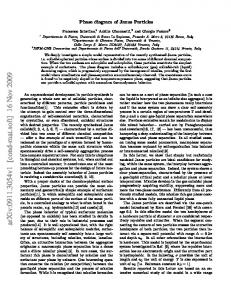
The “paramagnetic” state q
= 0 is everywhere a solution of (15). It is however numerically unstable above the line γuc = 1/ 4ǫ(1 − ǫ) (coinciding with the unit-clause upper bound). A non-paramagnetic q 6= 0 solution appears continuously above this line and is stable. Conversely, for ǫ < ǫ∗ , the non-paramagnetic ∗ solution appears discontinuously at connectivity γRS , and is a stable local attractor. ∗ ∗ ∗ The line γRS (ǫ), and even the “triple point” ǫ at which γRS (ǫ) touches γuc , depend on the choice ′ of Hamiltonian H (2) or H (13), and are plotted in fig. 3. Since the ground-state energy E(β → ∞) ∗ (11) is zero if and only if q = 0 we conclude that the line γRS for ǫ < ǫ∗ , and γUC for ǫ ≥ ǫ∗ is the replica-symmetric prediction for the SAT/UNSAT threshold.

9 FIG. 3: Results of the replica-symmetric cavity analysis and its stability. The continuous curves with no bullets are the rigorous bounds left for comparison. The line with diamonds corresponds to the replica-symmetric prediction for the SAT/UNSAT threshold derived from the Hamiltonian H, with Ea (+, +, +) = 1, while the line with triangles to the one derived from the Hamiltonian H′ , with Ea′ (+, +, +) = 2. The dotted line is the soft-fields instability of the replica-symmetric solution, it is separating the stable region (below) from the unstable one (above). For ǫ > 0.33 ± 0.02 the stability line seems to coincide with the SAT/UNSAT threshold. γ 2.0

0.2429 0.2277 0.2726 0.05

0.1

0.15

0.2

0.25

ǫ 0.3

0.35

0.4

0.45

UNSAT 1.875 (3) 1.861

Easy UNSAT

1.8

RS sat/unsat w. H RS sat/unsat w. H′ RS instability H

1.639 1.6

1.4

1.2

Easy SAT 1

There are striking hints towards the badness of the replica-symmetric solution. For example, the ∗ predicted critical value γRS (ǫ = 0) is different from the numerical one, and even larger than the rigorous upper bound. But there is also an inconsistency internal to the method. It is not possible that the satisfiability line in the phase diagram depends on the finite-temperature Hamiltonian used in the cavity ∗ equations, but the lines γRS coming from H and H′ are different. Another argument comes from the cavity prediction of the ground-state energy Emin = E(β → ∞) (11) which is zero if and only if q = 0. The discontinuous appearance of a new fixed point leads to a discontinuity in γ of Emin (γ, ǫ), but this is impossible, as we have the Lipschitz condition   ∂ Emin (γ, ǫ) ∈ 0, 31 ∂γ

(18)

coming from the fact that adding randomly M ′ clauses to an instance whose minimum energy is Emin can only give an instance with minimum energy in the range [Emin , Emin + M ′ ]. In section III E we will explain in detail why and where exactly the replica-symmetric solution breaks down. D.

The soft-fields analysis

In the region of the phase diagram where the RS hard-fields analysis predicts zero ground-state energy (SAT region) all the hard fields and biases are zero (g+ (0), g− (0) > 0 in the language of equation (14)). We denote with capital letters Ua→i and Hi→a the soft fields, i.e. ua→i = 0 +

Ua→i ; β

hi→a = 0 +

Their update is deduced analyzing the general cavity equations (7) X Hi→a = Ub→i ;

Hi→a . β

(19)

(20)

b∈∂ira


1 Jai Ua→i = − ln e2Jaj Hj→a + e2Jak Hk→a ; 2

(21)

10 Defining q(U ) and p(H) as the probability distributions of U and H over the graph, we have the selfconsistent equations p(H) = (1 − ǫ)˜ p(H) + ǫ p˜(−H) ; Z Y k k ∞  X X    γk Ui ; dUi q(Ui ) δ H − p˜(H) = e−γ k! i=1 i=1

(22) (23)

k=0

being the analogue of (15b), while for the (15a) one has q(U ) = (1 − ǫ)˜ q (U ) + ǫ q˜(−U ) Z 
 1 q˜(U ) = dHj dHk p(Hj ) p(Hk ) δ U + ln e2Hj + e2Hk 2

(24) (25)

These equations are already beyond the possibilities of an analytical treatment, and can be solved only by a population-dynamics technique [3]. In this “paramagnetic” region the expression for the RS ground-state entropy (logarithm of the number of SAT configurations) simplifies. Thus, knowing the distributions q(w) and p(g) we can compute the average entropy. In appendix B 1 we compute the average number of solutions hN i, annealed entropy ln(hN i), whereas the RS computation leads to quenched average of the entropy hln N i. The same quantity may be computed for a given large sparse graph from the message passing procedure (21). However, the result will be valid only in the region where the RS assumption is valid, see section III E. E.

The RS stability

The replica-symmetric solution will turn out to be incorrect if the assumption of having a single pure phase is proven to fail. As we know, a necessary condition for this is that fields incoming to a given node are uncorrelated. This property can be tested on the RS solution: if the spin-glass susceptibility diverges, then all the fields (and in particular the pairs of incoming ones) are strongly co-fluctuating, and the RS assumption is inconsistent. The (nonlinear) spin-glass susceptibility is defined as [29, 30] χSG (G) =

1 N

X

hsi sj i2c ;

χSG =

∞ X

(2γ)d E(hs0 sd i2c ) .

(26)

d=0

i,j∈V (G)

On the left is the definition for a fixed graph G, hsi sj ic is the connected correlation function between nodes i and j. On the right we consider the average over instances, in the thermodynamic limit, where sites s0 and sd are at distance d. The factor (2γ)d stands for the average number of neighbours at distance d, when d ≪ ln N . Assuming that the limit for large d of the summands in (26) exists (with the limit N → ∞ performed first), we relate it to the stability parameter :   d1 λ = lim (2γ) E(hs0 sd i2c ) . d→∞

(27)

Then the series in (26) is essentially geometric, and converges if and only if λ < 1. Using the fluctuation-dissipation theorem we relate the correlation hs0 sd ic to the variation of magnetization in s0 , caused by an infinitesimal magnetic field in sd . Then, one relates this quantity to cavity fields, i.e., up to a factor C independent from d, " 2 # X ∂ua→d 2 E(hs0 sd ic ) = C · E . (28) ∂ub→0 a∈∂d b∈∂0

Finally, using the fact that we perform the large-N limit first, the variation above is dominated by the direct influence through the length-d path between the two nodes, and this induces a “chain” relation: if the path involves the clause and variable nodes (ad , d, ad−1 , d − 1, . . . , a0 , 0) we have " d  2 # Y ∂u a →ℓ ℓ . (29) E(hs0 sd i2c ) = C · E ∂uaℓ−1 →ℓ−1 ℓ=1

11

{b ∈ ∂j r a}

{ub→j } hj→a j

a

k {c ∈ ∂k r a}

ua→i i

hk→a {uc→k }

Inside the paramagnetic phase and in the zero-temperature limit (but keeping soft fields of section III D), from (21), we have for a path like the upper one in the above figure Jai

∂ua→i ∂Ua→i −Jaj e2Jaj Hj→a = Jai = 2Jaj Hj→a . + e2Jak Hk→a ∂ub→j ∂Ub→j e

(30)

Instead of directly computing the stability parameter λ, it is equivalent, and numerically easier, to associate every bias ua→i in the population-dynamics algorithm with a positive number va→i . We update this number together with the fields according to X  ∂ua→i 2 X  ∂ua→i 2 va→i = vb→j + vc→k , (31) ∂ub→j ∂uc→k b∈∂jra

c∈∂kra

(we recall that, when performing population-dynamics technique, the labels “a → i” do not have any spatial meaning: the population is just a collection, and messages are randomly combined at each step). After equilibration, the numbers v will change on average geometrically, with a factor λ. Numerically, we see that for a given ǫ the stability parameter grows with connectivity γ. On fig. 3 we see the line above which the replica-symmetric solution is unstable (i.e. λ > 1). This line coincides with the unit-clause upper bound within the errors from about ǫ > 0.33 ± 0.02. In particular all the region where the RS results are contradictory is unstable. It is furthermore remarkable (and unexpected) that there exist a region in which RS solution is not stable, and yet the short clause heuristics a.s. finds a solution in polynomial time. IV.

1RSB CAVITY APPROACH AND ITS IMPLICATIONS FOR THE PHASE DIAGRAM

The understanding of the role of ergodicity in the validity of the replica-symmetric cavity assumption allows us to recast the cavity method as a more powerful tool, for the case in which there are (exponentially) many phases. The assumptions underlying this process go under the jargon term “1RSB” type of symmetry breaking [3, 4]. In the 1RSB approach we assume that exponentially many pure thermodynamical states (phases) exists, and that the neighbors of a node in absence of this node are uncorrelated only within each of these states. This happens because the cluster property (the small correlation of observables far from each other) holds only within a pure phase. The name replica symmetry breaking is due to historical reasons, since the mechanism was first proposed by Parisi [31], while using the “replica trick” in analysing a spin-glass model. The necessary but conceptually impossible handling of the multiplicity of pure phases may be replaced by a “survey” over these phases. The only memory of the original structure is through the free energies Fα of the various phases α. As the phases have to be weighted with a Boltzmann weight in Fα , a reweighting term has to be introduced in the “survey” equations, as we show in section IV A. In the zero-temperature limit the analysis leads to what are now called survey propagation equations, which are developed fully in section IV B. The solution to these equations is described in section IV C 1, in section IV C 2 are results of the stability analysis of this solution. Checking the validity of the 1RSB cavity assumption (1RSB stability analysis) gives us a hint if this solution could be the final correct one. This has been done for the K-SAT [11, 32] and Coloring problems [12] on random graphs. The results in those cases supported strongly the conclusion that the SAT/UNSAT thresholds computed with the 1RSB cavity method were exact. The 1RSB stability analysis is technically involved, we summarize the main steps in appendix D.

12 A.

General 1RSB cavity equations

We define a complexity function Σ(F ) as the logarithm of number of states, and hence it is computable by Legendre transform ∂Σ(F ) = βm ; ∂F

−βmΦ(m, β) = −βmF (β) + Σ(F ) ;

(32)

where the parameter m plays role of a second temperature, for free energies of states instead of energies of configurations, and is called the Parisi parameter of the replica symmetry breaking. The function Φ(m, β) is called the “replicated free energy”. Instead of one field and one bias on every edge, now we need to keep one field and one bias for every edge and every state. Or equivalently, as we assumed that there is a huge number of states, a distribution of fields and biases on every edge. The self-consistent equation for this distribution is [3, 4] Z Y Z Y −1 P a→i (ua→i ) = Za→i dub→k P b→k (ub→k ) dub→j P b→j (ub→j ) (33) b∈∂kra b∈∂jra
a→i · δ ua→i − F({ub→j }, {ub→j }) · exp(−βm∆F ).

The function F is the single-phase update of biases given by equations (7), and the last term is the reweighting of states, where ∆F a→i is the free-energy shift after adding clause a and all its neighbors except i. Referring to our calculations in equation (9a), this free-energy shift is e−β∆F

a→i

a→i a→i Y+1 + Y−1 Q b→j b→j j∈∂ari b∈∂jra (Y+1 + Y−1 ) 
 P si ,sj ,sk exp β hj→a sj + hk→a sk − E{Ja } (si , sj , sk ) Q Q = . j∈∂ari b∈∂jra (2 cosh βub→j )

= Q

Then, in analogy with (10), the replicated free energy Φ is calculated as X X (di − 1)∆Φi , Φ(m, β) = ∆Φa∪∂a − a

(34)

(35)

i

where di is the degree of the node i. The replicated free-energy shifts are Z Z i −βm∆Φa∪∂a −βm∆F a∪∂a −βm∆Φi e = e ; e = e−βm∆F .

(36)

The integrals are making R an average over Rthe distributions Rof the fields incoming to the cavity, similarly as in equation (33), i.e. f (u1 , . . . , uk ) = du1 P (1) (u1 ) · · · duk P (k) (uk )f (u1 , . . . , uk ). Since we are interested mainly in the ground-state properties of the ǫ–1-in-3 SAT problem, we need to take the zero-temperature limit. There are two standard ways of doing this The energetic T → 0 limit [4]: We take the limit β → ∞, m → 0 with y = βm fixed and finite. Then − yΦ(y) = −yE + Σ(E) .

(37)

Here we neglected the entropic contribution and we can obtain complexity as a function of energy. This is the 1RSB analog of the RS analysis with hard fields (warnings). The entropic T → 0 limit [33]: We take the limit β → ∞ at energy fixed to zero, E = 0. Then ˜ mΦ(m) = mS + Σ(S) ;

(38)

˜ where −βΦ(β, m) → Φ(m). Here we are fixed to zero energy, but on the other hand we can compute complexity (number of states) as a function of the state internal entropy. This is the 1RSB analog of the RS analysis with soft fields (beliefs).

13 In this paper we work out only the simpler energetic limit, the same as in [9] for K-SAT, or in [13] for Coloring. We will see how this analysis alone already gives us a large amount of information about the phase diagram. The reweighting (34) becomes in the zero-temperature energetic limit X X
∆E a→i = − max hj→a sj + hk→a sk − E{Ja } (si , sj , sk ) + |ub→j | + |ub→k | . (39) si ,sj ,sk

b∈∂jra

b∈∂kra

Since the fields h and biases u are integers, by relations (12), ∆E a→i also takes nonnegative integer values. In fact it counts the number of contradictions in one warning-propagation update. We want to determine whether a typical ǫ–1-in-3 SAT instance has any satisfying configuration. We do this in section IV B, by taking the y → ∞ limit. The reweighting term exp (−y∆E a→i ) then guarantees that we keep only the cases without contradictions, ∆E a→i = 0. Conversely, in order to compute the ground-state energy in the UNSAT region, or the complexity at energies higher than zero, we need to keep y finite. We undertake this in appendix C. B.

The zero-energy case, survey propagation

In the limit y → ∞ we fix the energy to be zero. The energy shift ∆E a→i is zero if and only if: • The {ub→j }b∈∂jra are all nonnegative or all nonpositive, • The {ub→k }b∈∂kra are all nonnegative or all nonpositive, P P • The terms Jaj b∈∂jra ub→j and Jak b∈∂kra ub→k are not both positive.

We begin by simplifying the form of eq. (33). In the zero-temperature energetic limit we can write the distribution of fields and biases over states on every edge as a→i a→i P a→i (ua→i ) = q− δ(ua→i + 1) + q+ δ(ua→i − 1) + q0a→i δ(ua→i ) ;

P

i→a

(hi→a ) =

i→a p− µ− (hi→a )

+

i→a p+ µ+ (hi→a )

+

p0i→a δ(hi→a ) ;

(40) (41)

i→a i→a a→i a→i + p0i→a = 1, and µ± (h) are normalized measures with support + p+ + q0a→i = p− + q+ where q− over Z± . So, to every oriented edge we associate a triple of numbers q = (q− , q0 , q+ ) or a triple p = (p− , p0 , p+ ) (resp. if oriented towards the variable or the clause). In analogy with the self-consistent equations (7) for fields and biases we can write self-consistent equations for probabilities (surveys) q and p.

{b ∈ ∂j r a}

q b→j pj→a

q a→i

j

a

k

i

pk→a {c ∈ ∂k r a}

q

c→k

Considering only the combinations with ∆E a→i = 0, the surveys of fields are given by incoming surveys of biases as Y −1 i→a a→i p+ + p0i→a = Ni→a (q+ + q0a→i ) ; (42a) b∈∂ira

i→a p−

+

p0i→a

=

−1 Ni→a

Y

b→i (q− + q0b→i ) ;

(42b)

b∈∂ira −1 p0i→a = Ni→a

Y

b∈∂ira

q0b→i ;

(42c)

14 where Ni→a is the normalization factor (in the update, we have three equations for three independent unknown, p± and N ). And the surveys of biases are given by the incoming surveys of fields −1 k→a = Na→i pj→a qJa→i −Jaj p−Jak ; ai a→i q−J ai

=

−1 Na→i

pj→a Jaj (1

−

(43a)

pk→a Jak )

+ (1 −


k→a pj→a ; Jaj )pJak

j→a −1 k→a q0a→i = Na→i pj→a + pj→a pk→a p0 −Jak + p0 0 −Jaj p0

(43b)


k→a

;

(43c)

where Na→i is the normalization factor, and the lower indexes of q’s and p’s are multiplied by −1 when variable is negated in the clause. These equations describe survey propagation [9], and can be used inside an algorithm to find a solution to a typical instance of ǫ–1-in-3 SAT, hopefully also in a region of parameters (ǫ, γ) where short-clause–like heuristics or belief-propagation methods fail. They might also be used to compute quantities averaged over instances in our random ensemble, particularly the complexity function which determines the SAT/UNSAT transition. In the zero-temperature limit, the replicated free energy (35) becomes Z   X X Z −y∆E i −y∆E a∪∂a (di − 1) ln , (44) − yΦ(y) = ln e − e a

i

where from (9) and (36) we get the energy shifts ∆E a∪∂a = − max

si ,sj ,sk


X X hi→a si + hj→a sj + hk→a sk − E{Ja } (si , sj , sk ) + |ub→i | ;

(45)

i∈∂a b∈∂ira

X X ∆E i = − ua→i + |ua→i | ; a∈∂i

(46)

a∈∂i

again both these energy shifts are non-negative integers. Furthermore in the y → ∞ limit, we distinguish only if ∆E = 0, then exp(−y∆E) = 1, or if ∆E > 0, then exp(−y∆E) = 0. From eq. (44) we get for the complexity at zero energy X
X
Σ(E = 0) = ln prob(∆E a∪∂a = 0) − (di − 1) ln prob(∆E i = 0) , (47) a

where, calling

P0i

:=

i

a→i a∈∂i q0

Q

and

i P±

:=

a→i a∈∂i (q±

Q

+ q0a→i ),

i i prob(∆E i = 0) = P+ + P− − P0i ; Y Y Y i→a i→a prob(∆E a∪∂a = 0) = − P0i→a ) − + P−J (PJi→a − P0i→a ) − (P−J − P0i→a ) (PJi→a ai ai ai ai i∈∂a

−

X

i∈∂a

i→a P−J ai

i∈∂a

Y

(PJj→a aj

−

P0j→a ) .

i∈∂a

(48a)

(48b)

j∈∂ari

The second equation collects the contributions from all combinations of arriving fields except the “contradictory” ones (+, +, +), (−, −, −), (+, +, 0) and (+, +, −) (plus permutations of the latters). Note at this point that all these equations (42)-(48) correctly do not depend on the choice of Hamiltonian (2) or (13). C.

1RSB results for the phase diagram

In this section we give results of 1RSB cavity analysis for the ǫ-1-in-3 SAT problem. In the first two subsections we concetrate on the positive 1-in-3 SAT (ǫ = 0). In the third one IV C 3 we show results for general probability of negation. 1.

Complexity as a function of connectivity

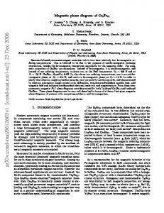
To compute numerically the average value of complexity from eq. (47) we first need to find a fixed point of the survey propagation equations (42) and (43). We do that using the population-dynamics algorithm [3]. The result is in fig. 4.

15 Σ/N 1.8 1.822 1.85 1.879 1.9 0.004

1.992

γ symbol popul. size

0.002

+

0



-0.002 -0.004

1.95

◦ 1.875 1.8789

1.885 0.0005

0.5 × 105 1.0 × 105 2.0 × 105

-0.006 -0.008

0

-0.010 -0.0005 -0.012

FIG. 4: Average complexity density (logarithm of number of states divided by size of the graph) as a function of mean degree γ for the positive 1-in-3 SAT problem. At γsp = 1.822 a nontrivial solution of survey propagation equations appears, with positive complexity. At γ = γ ∗ = 1.8789 ± 0.0002 the complexity becomes negative: this is the SAT/UNSAT transition. At γp = 1.992 the solution at zero energy ceases to exist. The inset magnifies the region where the complexity crosses zero, together with the error bar for the SAT/UNSAT transition.

Below mean degree γsp = 1.822 ± 0.001 the survey propagation equations (42, 43) have only the trivial paramagnetic solution, with p0 = q0 = 1 and q± = p± = 0 for all edges. At γsp a solution of survey propagation equations with positive complexity appears discontinuously. The emergence of this transition far below the numerically known SAT/UNSAT threshold suggests that, in a whole interval of parameters near to the threshold the phase space restricted to solutions is clustered into many pure states, a HardSAT phase [9] exists. Furthermore, in that interval, there are also many metastable states, entropically relevant, and local minima with positive energy cost separated by macroscopic barriers. This means that local algorithms, like decimation heuristics or variants of annealed Monte Carlo, get trapped and are unable to find any ground state in polynomial time. Nonetheless, a decimation procedure based on the stationary distribution of survey propagation equations is expected to work beyond this threshold. Note that γsp is referred to as a “dynamical threshold” in [9, 13], we stress that it is not this point which is connected to a real dynamical transition [34]. Neither is it the point where the local algorithm ceases to work in polynomial time. We come back to comment about this point in the discussion, section V. At mean degree γ ∗ = 1.8789 ± 0.0002 the complexity becomes negative. Instead of having a.s. in each instance an exponential number of clusters which contain at least one solution, the fraction of instances having any cluster which contains at least one solution (i.e. the fraction of SAT instances) becomes exponentially small. So this point identifies the SAT/UNSAT transition. We are aware of two works where results from numerical simulation for this SAT/UNSAT threshold are given. In [22] they conclude the value of threshold is γ ∗ = 1.86 ± 0.03. In [23] they give γ ∗ = 1.875 ± 0.015. In fact, the latter do not give an error bar, so we guessed it from their fig. 4. Our result agrees with these estimations, and as it is based on an analytical method we reduce the error bar by one order of magnitude with a very small numerical effort. At mean degree γp = 1.992 ± 0.001 the solution at zero energy ceases to exist. In the y → ∞ limit the population dynamics converges to a solution which shows a finite fraction of surveys of type (p± , p0 , p∓ ) = (0, 0, 1). Then, with finite probability we would find two such surveys creating a contradiction, the normalization in (43) then would be zero. We call this situation a “hard contradiction”. Note that such a phenomenon does not occur in K-SAT or Coloring problems. Cavity equations deal with the messages incoming to a clause from all neighbours but one. In both K-SAT and Coloring (and in many other problems, like NAE-K-SAT, Vertex Covering, and so on), there is no way of making a clause unsatisfied if one of the neighbouring variables is not restricted, and indeed a γp threshold has never appeared in the cavity analysis for these systems. In order to obtain a non-singular solution above connectivity γp , we need to work with the equations at finite y, which is able to account for the positive energy contributions. The results of the finite y analysis are shown in appendix C 1.

16 2.

ln µII

The stability analysis

γ=1.825

µI 1.04

0.1

1.03

0

γ

1.83

1.85 γ=1.83

−0.1 1.0

1.01

d ln µII (d) 0.5

γ=1.835

1 0.99

0 γ=1.84

0.98

γ=1.845

0.97

−0.5 −1.0

1.02

4

8

12

16

d γ=1.85

0.96

1.93

1.94

1.9475

1.95

1.96

γ

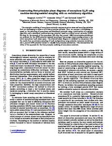
FIG. 5: The stability parameter of the second kind ln(µII (d)) (D3) for positive 1-in-3 SAT for different connectivities as a function of length of the chain d. When the slope is negative, the 1RSB at this connectivity is stable against bug proliferation, and vice versa. This happens for γ > γII = 1.838 ± 0.002. Right: The stability parameter of the first kind µI (D9) as a function of connectivity for positive 1-in-3 SAT. The stability parameter is smaller than 1 for γ < γI = 1.948 ± 0.002, for these connectivities the 1RSB equations are stable against noise propagation.

In appendix D we introduce two stability parameters µI (D9) and µII (D3). Their meaning is analogous to that of the replica-symmetric stability parameter λ (27). The 1RSB solution is stable if and only if both µI < 1 and µII < 1. The results for stability parameter of the second kind µII (D3) for positive 1-in-3 SAT are shown in fig. 5 (left), for finite d. Extrapolation to d → ∞ is done by linear fit, which looks reasonable from the data points. So our criterion is that, if the slope in the logarithmic plot is positive, the limit value µII is larger than 1, and vice versa. We estimate that 1RSB is “type-II” stable for γ > γII = 1.838 ± 0.002. More directly, for the stability parameter of the first kind µI (D9), the results are shown in fig. 5, right. So we get that 1RSB is “type-I” stable for γ < γI = 1.948 ± 0.002 (the generous error estimate is due to potential biases caused by finite population sizes). The 1RSB solution may be correct only if both the stability parameters are smaller than one. For positive 1-in-3 SAT this happens for connectivities in the range 1.838 ≃ γII < γ < γI ≃ 1.948. So, in particular, the SAT/UNSAT threshold γ ∗ is in the range of stability, and its value is to be considered exact. Note that such a situation, in which the SAT/UNSAT threshold falls into a narrow stability region, is quite common, and it has been seen also in K-SAT [11] and Coloring [12]. 3.

1RSB results for general probability of negation

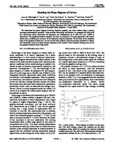
We applied the techniques of section IV C to the problem at finite ǫ. As expected, all the critical connectivities describe curves which are continuous at ǫ = 0. We thus show, in figure 6 (left), the curves γ ∗ (ǫ), γsp (ǫ) and γp (ǫ), and, in the magnification on the right of fig. 6, also γI (ǫ) and γII (ǫ). As ǫ approaches about 0.20, the interesting interval γsp < γ < γp becomes very narrow (fig. 6, right), and the complexity value very small, Σ ≈ 10−5 , three orders of magnitude smaller than the analogous values for ǫ = 0. Above ǫ = 0.20 we do not have sufficient numerical resolution to examine this region at all. ∗ In fig. 6 (right) we plot the four curves γsp (ǫ), γp (ǫ), γI (ǫ) and γII (ǫ), shifted by the
curve γ (ǫ), which
is used as a reference. This allows us to appreciate that the differences γ ∗ − γsp (ǫ) and γp − γ ∗ (ǫ) seem to vanish linearly at about ǫp = 0.21 ± 0.01, these two linear fits extrapolating to the same value of ǫ with reasonable confidence. Above ǫp , as soon as a nontrivial solution of (energetic finite-y) 1RSB cavity equations exists, it has immediately a complexity Σ(E) of the qualitative shape for the connectivities above γp , (for example see fig. 8 in appendix C). We are thus led to conclude that in this interval the line γp (ǫ) should be taken as the 1RSB prediction for the SAT/UNSAT line γ ∗ (ǫ). At about ǫ = 0.26 ± 0.01 the curve γp (ǫ) joints the unit-clause upper bound.

17 We should add that, above ǫ ≃ 0.07, both stability criteria fail along the curve γ ∗ (ǫ) (and then, along γp (ǫ), for ǫ > ǫp ), so that the 1RSB prediction for the SAT/UNSAT transition is not expected to be exact, but only an upper bound, in the range 0.07 < ǫ < 0.2726 [35, 36]. γ − γ ∗ (ǫ)

γ

0.10

2.0 γp =1.992

UNSAT

Easy UNSAT

γ ∗ =1.8789

0.05

γsp =1.822 1.8 0 γsch =1.639 1.6

ǫ

−0.05 0.05

0.10

0.15

0.20

stable 1.4

γ ∗ (ǫ) γp (ǫ) γsp (ǫ)

Easy SAT

1.2 0.05

0.07

0.1

0.15

0.2

0.21

0.25

0.2726

0.3

0.35

ǫ

γI (ǫ) γII (ǫ)

FIG. 6: Left: plot of the three curves γ ∗ (ǫ), γsp (ǫ) and γp (ǫ) described in the text. We left for comparison the SCH lower bound (dot-dashed curve) and the RS instability line (dotted curve with stars data points). Right: The same data, with connectivity plotted with respect to the SAT/UNSAT threshold prediction γ ∗ (ǫ). Also the stability lines γI (ǫ) and γII (ǫ) are shown, and the interval of stability for the SAT/UNSAT curve is ǫ ∈ [0, 0.07 ± 0.01]. In the inset, all the error bars are approximately as big as the point size.

V.

DISCUSSION AND CONCLUSIONS

We studied the average-case behaviour of 1-in-3 SAT in the random ǫ–1-in-3 SAT ensemble, where ǫ ∈ [0, 1/2] is the probability of negation. This generalizes the random (symmetric) 1-in-3 SAT problem (ǫ = 1/2) and random positive 1-in-3 SAT problem (ǫ = 0), which is a special ensemble of Exact Cover. Our main result is the phase diagram in fig. 1, and, magnified, in fig. 6 above. It fills the conceptual gap between the symmetric problem, of polynomial average-case complexity both in the SAT and UNSAT regions, and the positive problem, which shows a Hard-complexity phase around the SAT/UNSAT threshold. Concerning the SAT/UNSAT transition curve, γ ∗ (ǫ), we computed upper bounds coming from unitclause technique (UC), and from first moment method with restriction to the 2-core (1MM), and the lower bound coming from short clause heuristics (SCH). The UC and SCH bounds have been proven to coincide on the interval ǫ ∈ [0.2726, 1/2], and thus determine the corresponding portion of the SAT/UNSAT line rigorously. All the other results are obtained with the non-rigorous cavity method. The results of the replicasymmetric calculations do not give us a better result for the SAT/UNSAT threshold than the UC and SCH bounds, since its prediction have to be rejected above the RS stability line γRS , fig. 3. It is remarkable that a region of the phase diagram exists, where the replica symmetry is broken, while the short clause heuristics is proven to succeed a.s. in polynomial time. For what we know, such a feature has not been proven in any of the previously studied models, while it has been often observed empirically that some local algorithms, e.g. the Walk-SAT [37, 38, 39, 40], works in linear time inside a phase with replica-symmetry breaking. We are tempted to say that this result actually proves that the onset of a non-trivial replica symmetry broken solution does not imply to the onset of computational hardness (unfortunately the cavity results are not rigorous and the term “computational hardness” would have to be defined properly to be allowed to speak about a proof). However, we hope that this could be used to study in a new way the nature of the replica-symmetry-broken phase. On the other hand, and as claimed before, we are persuaded that a stable 1RSB solution suggest an existence of a Hard-SAT phase near to the SAT/UNSAT transition (nearer than the stability threshold). For quantitative study of this point for

18 the coloring problem see [41]. The analysis of [41] should be repeated for 1-in-K SAT problem in future works. Our main insights for the region with ǫ < 0.2726 comes from the one-step–Replica-Symmetry-Breaking (1RSB) calculations by analsis of the energetic zero-temperature limit of the 1RSB cavity equations (33), in which we keep only the weights of the hard fields instead of whole probability distribution. For ǫ < 0.21 we can locate, on the curves for the zero-energy complexity function Σ(γ) fig. 4, the connectivities γ ∗ (ǫ) at which Σ vanishes, this corresponding to the SAT/UNSAT transition. The same computation shows the existence of a nontrivial solution above γsp (ǫ) < γ ∗ (ǫ), thus predicting a whole interval of Hard-SAT phase with many pure states. However for exact location of the “dynamical transition” we would need to keep the information about the soft fields and compute when a nontrivial solution of eq. (33) appears for the entropically dominating clusters, see [34]. Note here also that the inequality γsp < γRS for small ǫ is due to the discontinuity of the transition towards nontrivial 1RSB phase, that can not be seen by the local RS stability analysis. Analysis of [34] would also show that a nontrivial 1RSB solution exists everywhere in the region of γ > γRS . This analysis for 1-in-K SAT might be a direction for future work. Above the line γp (ǫ), fig. 6, the system shows a transition to a phase where the 1RSB solution at zero energy ceases to exists, while it still exists above some value Emin (γ, ǫ). This is due to the presence of hard contradictions, a phenomenon specific of strongly constrained problems, like 1-in-K SAT, and to our knowledge it is a newly observed fact. Interpretation of this transition may be that the SAT formulas start to be subexponentially rare at the connectivity γp . For ǫ > 0.21 the nontrivial 1RSB solution at zero energy never exists, and we can trace only the curve γp . This would be the 1RSB prediction for the SAT/UNSAT transition. This result suggests that for ǫ > 0.21 a Hard-SAT region might actually be absent. Specifying what sort of replica-symmetry-broken solution is connected with the breakdown of local algorithms, like decimation heuristics or variants of annealed Monte Carlo, is an important direction of future research. We have checked the local stability of 1RSB solution towards 2RSB. The result is that 1RSB is stable only in a small region between the lines γI and γII in fig. 6. This means, among other things, that the 1RSB location of the SAT/UNSAT transition for ǫ < 0.07 is likely to be exact. In particular, this is true for the positive 1-in-3 SAT threshold, γ ∗ = 1.8789. For 0.07 < ǫ < 0.2726 the 1RSB result is unstable so the exact location of the SAT/UNSAT transition in that region remains an open question. We can only conjecture that our 1RSB result is an upper bound, in analogy with proofs for other models in [35, 36]. Furthermore, it would be interesting to compare our results with the behaviour of the structurally affine (2 + p)-SAT problem [16, 17] for which the 1RSB analysis is still missing. Finally, as we mentioned in several places above, the 1RSB cavity approach allows for algorithmic implementations. We started studying this aspect also together with Elitza Maneva and Talya Meltzer, and the results will be published elsewhere. Acknowledgments

We thank the organizers of the “Complex Systems” July ’06 Les Houches Summer School (Session 85), where this work has been started. This work has been supported in part by the EU through the network MTR 2002-00319 “STIPCO” and the FP6 IST consortium “EVERGROW”. A.S. also thanks the LPTMS of Orsay – Paris Sud for support and kind hospitality in large stages of the work. We thank also Elitza Maneva and Talya Meltzer for collaboration in some still unpublished algorithmic parts of this work. We appreciated a lot discussions with Florent Krz¸akala, R´emi Monasson and last but not least we thank Marc M´ezard for his precious hints. APPENDIX A: UPPER AND LOWER BOUNDS FROM UNIT-CLAUSE PROPAGATION AND DECIMATION HEURISTICS

Consider an instance drawn from an appropriate ensemble, and subject to a decimation algorithm wherby in each time set a variable is set to ±1. Call X the discrete decimation time (number of variables set, among the N total) and Ci (X) the number of clauses remaining of length i ≥ 2. Thus the initial conditions for the instance are X = 0 and Ci (X) = N γ3 δi,3 . Assume for now these quantities are sufficient to describe the instance in the absence of clauses of “length 1” (unit clauses). If we assume a variable is fixed (decimated) from such an instance, the remaining instance involves a smaller number of literals,

19 so it is simplified in some respect. More importantly, some of the clauses are shortened, and may even be reduced to unit clauses. The unit clauses, being only 1 literal, allows no ambiguity in the values their variables must take in order for the instance to be SAT. The initial fixing of one variable by this process, forces the value of some other variables, which may again propagate, i.e. a branching process. So, a single binary choice could decrease the number of variables by a considerable amount, as a result of a cascade of these unit-clause implications. The justification in considering the instance at all times described by {Ci (X)} and X is the following. For sufficiently simple decimation rules, the distribution of remaining variables within clauses will be uniform and random at all X, and if N is sufficiently large the values of Ci (X) are self-averaging. Furthermore, at fixed clause length, the fraction of clauses with a given number of negations is the one expected
from an independent Bernoulli process: among clauses of length i, at all times there is a fraction hi ǫh (1 − ǫ)i−h of clauses with h negations. All these elements are necessary to allow a sufficiently concise dynamical description to make the progress in the following sections. Among the various possible heuristics – which determine the values set in the absence of unit clauses, one typically is interested in the (suboptimal) subset of heuristics which preserve these decorrelation properties of the Poissonian ensemble, so that a statistical analysis is achievable. It is useful to consider the algorithm as partitioned into rounds, which consist of a single application of the heuristic rule (free step), followed by the cascade of unit-clause propagations (forced steps). In expectation, the number of variables fixed throughout a round of unit-clause propagation is described by a transition matrix depending on the clause distribution {Ci (X)}, which are constant to leading order during any “subcritical” round (defined below). The unit clauses generated in the first free step go on to generate other unit clauses and so forth, this can be described by a geometric series in the transition matrix M(X). Calling p = (pT , pF ) and m = (mT , mF ) respectively the expectations for the numbers of variables fixed to (True, False) at the first level of the cascade (p), and on the whole cascade (m), we have m = p + M(x)p + M2 (x)p + · · · = (I − M(x))−1 p .

(A1)

The matrix inverse above is justified from the fact that, for consistency of the approximations, we require the round to be subcritical, thus we must consider the range of parameters where the modulus of the largest eigenvalue of M is smaller than 1. This is also responsible for the approximation that M(x) remains invariant (up to order N1 ) during the cascade. The transition matrix has two components. A first one comes from K-clauses which are “broken” into a bunch of K − 1 unit-clauses, because the fixed variable already satisfies the original one, and all the other K − 1 variables thus should take the value not satisfying the clause. A second one comes from 2-clauses (if any) which were just “shortened” because although the fixed variables are not satisfying them, the left over variables must, by definition creating unit clauses. Since there are Ci (x) clauses of length i and N − X variables left in the instance, these two terms are combined in the expression " ! !# 2 ǫ(1 − ǫ) ǫ2 ǫ(1 − ǫ) (1 − ǫ)2 M(x) = (C2 (X) + 3C3 (X)) + C2 (X) . (A2) N −X (1 − ǫ)2 ǫ(1 − ǫ) ǫ2 ǫ(1 − ǫ) Here we identify that the unit-clause cascades on a large graph are a simple uncorrelated process, governed by the spectrum of a certain finite-size “transition matrix” (in our case, 2 × 2). If all the eigenvalues have |λi | < 1, the process is subcritical : the typical size of the cascades is ∼ 1/ mini (1 − |λi |), and their average size concentrates. Conversely, when the gap 1 − |λi | vanishes, a single cascade could visit a finite fraction of a graph even in the large N limit, and thus could lead to a contradiction. Also note that both the upper- and lower-bound arguments later derived are complemented by an analysis of the concentration properties of the process [21], and by a non-rigorous argument on the approximate decorrelation of distinct random restarts on a fixed instance. The vulgate version reads: “If a random algorithm succeeds with finite probability p on its first run, after ∼ n independent runs the probability of success will be ∼ 1 − exp(−n ln(1 − p) + · · · )”, where the dots stand for some function of the correlations, small in n/N , caused by working with a fixed finite instance. We do not discuss here these complex technical points. 1.

Upper bound

If, for a variable i selected randomly from the initial instance, both the cascades initiated by s(i) = +1 and s(i) = −1 percolate, there is a finite probability that they result in a certificate of contradiction.

20 Thus the upper bound for the SAT/UNSAT transition comes from the requirement that the cascades are on the edge of criticality already at time X = 0. At this point we have C2 = 0 and C3 = N γ/3, so that we get !

ǫ(1 − ǫ) ǫ2 M(0) = 2γ −→ λ1 , λ2 = 4γ ǫ(1 − ǫ), 0 . (A3) 2 (1 − ǫ) ǫ(1 − ǫ) From this we see that a random instance is a.s. (randomized linear time) provable to be unsatisfiable for γ larger than the percolation threshold γuc (ǫ) =

2.

1 . 4ǫ(1 − ǫ)

(A4)

Lower bound

The differential equations studied here are a generalization of those found by Kalapala and Moore [22] for the case of positive 1-in-K-SAT. The heuristic determines the nature of the free step in our rounds. The two rules examined here in are random heuristic (RH[p]) and short clause heuristic (SCH). In RH[p] a variable is chosen at random, with uniform probability, from the remaining unassigned variables and set to true with probability p. In SCH, a random 2-clause is selected (if any exists) and a random literal set to satisfy the clause (hence the other literal is set to not satisfy it). If at some time no 2-clauses exist, a RH choice is performed, but fact will not be relevant in our statistical analysis: criticality of the cascade process will always arise after a time interval throughout which an extensive number of short-length clauses have been present (except at X = O(1)). If at some time X, pT variables are set to True and pF to False in expectation, then Ci changes accordingly. If an i-clause contains the variable just fixed, it is reduced to an (i − 1)-clause, and similarly an (i + 1)-clause can be reduced to an i-clause. Call ǫ = (ǫ, 1 − ǫ), p = (pT , pF ), and 1 = (1, 1). Still in expectation:  
i i+1 Ci (X + 1 · p) = Ci (X) − aδi,2 (1 − δC2 (X),0 ) 1 − (1 · p) + (ǫ · p) Ci+1 (X) ; (A5) N −X N −X where a = 0 or 1 respectively in the case of RH[p] and SCH. The two heuristics are distinguished in that to initiate the cascades for RH[p] we have pRH[p] = (p, 1 − p), and for SCH we have pSCH = (1, 1). The SCH value can be understood since setting one random literal in a two clause implies setting the other to the opposite value, thus setting variables to either ±1 is equally likely in expectation. A round can be described by incorporating the variables set in the forced steps. Suppose that during a subcritical round mT variables are set to True and mF to False in expectation (including the free step), and call m the vector (mT , mF ). To leading order in N − X the variation is  
i+1 i (1 · m) + (ǫ · m) Ci+1 (X) , (A6) Ci (X + 1 · m) = Ci (X) − aδi,2 (1 − δC2 (X),0 ) 1 − N −X N −X

A final simplification in the clause dynamics is to summarize the behavior by continuous variables x = X/N and ci = Ci /N . In the hypothesis of subcriticality, m/N is infinitesimal, and we attain a differential equation description   Dǫ · mE  d 1  1 + −ici (x) + (i + 1) ci+1 (x) , (A7) ci (x) = −aδi,2 θ(c2 (x)) dx 1·m 1−x 1·m For both RH[p] and SCH rules, the equation for c3 (x) gives c3 (x) =

γ (1 − x)k , 3

(A8)

Instead, for c2 (x) the equation is nonlinear. Indeed we get that hmT i and hmF i are given by the combination of equations (A1, A2, A8), and thus depend on the unknown function c2 (x) (besides, of course, x,

21 FIG. 7: On the left, profiles of λ(x) along decimation time x, for RH[1], at various ǫ and at the corresponding critical value of γ. In all the cases, the functions λ(x) are concave (up to the limit value ǫ = 1/2, where λ(x) = 1 − x). For ǫ larger or smaller than the tricritical value ǫ∗ = 0.272633, the maximum of λ(x) is achieved respectively at x = 0 or at x > 0. On the right, critical curves γsch (ǫ) and γRH[1] (ǫ), obtained through short-clause (SCH) and random heuristic at optimal parameter p = 1 (RH[1]). For a comparison with other values and curves here out of range, cfr. figures 1, and 3. λ(x) 1

γ

0.8 0.6

1.639 1.603

ǫ=0

γsch γuc = γrh[1]

ǫ = ǫ∗

1 4ǫ(1−ǫ)

1.4

ǫ = 0.5 0.4

1.261 1.2

0.2 0.2

0.4

0.6

0.8

1 x

ǫ 0

0.1

0.2

0.3 0.272633

ǫ and γ). Using this expression within (A7) allows us to determine c2 (x) by numerical integration, and thence λmax (x). The best choice for the parameter p in RH[p] is the one which creates the smallest cascades, i.e. the one “more orthogonal” to the principal eigenvalue ǫ = (ǫ, 1 − ǫ), but compatible with the probabilistic interpretation of p. Thus, in the whole interval ǫ ∈ [0, 1/2], the choice p = 1 is optimal. Here we thus show the results for RH[1] and for SCH. The latter is always at least as good as the former, and gives a lower bound of γsch = 1.6393, while RH[1] attains γrh = 1.6031, for the case ǫ = 0. Kalapala and Moore calculated these quantities for positive 1-in-K SAT, with compatible results for the K = 3 case (up to maybe a misprint exchanging RH[p] with RH[1 − p]). 3.

Exact SAT/UNSAT threshold for ǫ > 0.2726

This section proves the coincidence of the curves γsch (ǫ) and γuc (ǫ) for ǫ > 0.2726. It was shown in the previous section that whenever the cascades remain subcritical we are in the Easy-SAT phase. The criteria for the cascades to be subcritical at x = 0 is precisely γ < γuc (ǫ). It thus suffices to show that the maximum (over the decimation time x) of the maxi |λi (x)|, is attained for x = 0. This is indeed what happens in the interval ǫ ∈ [0.2726, 1/2]. Building on the previous section we will see that, for ǫ–1-in-3-SAT and our heuristics, λ(x) is a concave function. So, the interval on which γuc (ǫ) and γsch (ǫ) coincide is the one in which dλ(x; ǫ, γ = γuc (ǫ)) ≤ 0, (A9) dx x=0

the endpoint being determined by the corresponding equality. It is possible to calculate the characteristic polynomial (and differentiate w.r.t. x). The expressions thereby found can, however, only be evaluated exactly at x = 0. At this value we have expressions for ci (x) and there derivatives in terms of the initial conditions and m. As we increase connectivity towards the critical limit, 4γ ǫ(1 − ǫ) = 1, a further simplification is in the eigenvectors of M which become ǫ and its orthogonal, the latter having null eigenvalue. Regardless of p (which must have a component along ǫ in order to have positive components), we have ǫ·m ǫ·ǫ F (x, ǫ) := ; F (0, ǫ) = = 1 − 2ǫ(1 − ǫ) . (A10) 1·m 1·ǫ Finally, the condition (A9) becomes  2 ! ǫ 1−ǫ 1 (1 − 2ǫ(1 − ǫ)) − 2 ≤ 0 . + 1+ 4 1−ǫ ǫ

(A11)

22 So that finally, after the change of variable x = 2ǫ(1 − ǫ), one gets the equation for the endpoint of the interval 2x3 − 2x2 + 3x − 1 = 0 ,

(A12)

whose only real solution gives ǫ = 0.272633, or its symmetric point. To show that the properties at x = 0 are sufficient to determine γsch it is necessary to show that whenever criteria (A11) is met, and λ(0) < 1, the algorithm is subcritical at all x. If we want a true ˆ analytic proof, besides the numerical evidence of figure 7 (left), a method is to find a function λ(x) such that ˆ λ(x) ≤ λ(x) ≤ λ(0) ,

(A13)

hence establishing the result. Since we find that λ(x) is a monotonically increasing function of c2 (x), an upper bound cˆ2 (x) > c2 (x) ˆ implies an upper bound in λ(x) also which we take to be λ(x). The bound function cˆ2 is defined by replacing the complicated function F (x, ǫ) by the constant value F (0, ǫ) in the expression (A7), which are then exactly solvable for all x as
(A14) cˆ2 (x) = γx(1 − x)2 F (0, ǫ) = γx(1 − x)2 1 − 2ǫ(1 − ǫ) .

For RH[ 12 ] and certain other heuristics this approximation can be shown to produce an upper bound for c2 (x), and yet be exact at x = 0 in both absolute value and derivative. ˆ

This then allows an exact expression for dλ(x) dx to be written in terms of x. Though the dependency on x remains complicated it can be established that ˆ dλ(x) 3 the curves are not convex for some ǫ; the gradient at x = 0 may be negative and yet the global maximum in lambda appears at x > 0. On first inspection a rigorous bound appears more challenging to obtain in these cases. APPENDIX B: OTHER BOUNDS 1.

Upper bound from first moment method

Here we obtain the statistical properties of the 2-core of random bipartite graphs, in the Erd¨ os-R´enyi ensemble described in section I A, with K = 3. Assuming γ > 1/2, the percolation transition, we solve self-consistently for the probability that a given branch of the graph is not percolating. We use “giant” or “small” for synonymous of “of size of order N ” or “of size of order 1” respectively. Indeed, for graphs in our ensemble, a.s. there is a single giant 2-core component. Each edge is either attached on both sides to a small tree; is attached to a small tree on one of the two extrema, and to the giant 2-core on the other one (i.e. it is in the leaf-part of the giant component); or is connected to the 2-core through both extrema. Only in this last case is it in the 2-core of the graph. Consider an incoming edge from a clause on the original graph. Call q the probability that the part of the graph “downstream” is a tree. The edge will be attached to a variable, participating in k other clauses (k Poissonian distributed of rate γ). For each clause there will be two incoming edges, which must also be connected to finite trees. Self-consistency will thus require that q=

X k

e−γ

2 γ k 2k q = e−γ(1−q ) . k!

(B1)

The two functions q(γ) and γ(q), inverse of each other, are both monotonic on our domains q ∈ [0, 1], γ ∈ [1/2, +∞). In particular, γ(q) has an algebraic form γ(q) = −

ln q 1 − q2

(B2)

23 so that using q as a parameter instead of γ will simplify our equations. The probability that an incoming branch from a variable is connected to a tree is q 2 , as it is the probability that both outgoing branches from the neighbouring clause are connected to a tree. Thus, the average number of variables of coordination k ≥ 2, hNk i, is proportional to a Poissonian with rate γ(1 − q 2 ) = − ln q. Then, there will be hM3 i = (1 − q)3 M clauses remaining of degree 3, and hM2 i = 3q(1 − q)2 M clauses reducing to 2-sat clauses, all the others are decimated by the leaf removal. The P number of edges is E = k kNk = 3M3 + 2M2 , so on average hEi = N (− ln q)(1 − q). All these averaged quantities are concentrated. Consider the ensemble of configurations s, in “spin” notations as in the rest of the paper. Call xk the fraction of variables of degree k which take value +1: the space of configurations is thus described by the infinite vector {xk }k≥2 , with each x in [0, 1], and a vector {xk } comes with an entropy X Svar (~x) = Nk h(xk ) , (B3) k

where we use the common two-state entropy function h(x) = −x ln x − (1 − x) ln(1 − x). Denote by x the fraction of incoming edges from variables assigned value +1 1 X x= kNk xk , (B4) E k

and by p the fraction of edges (ai) such that Jai si = +1, and hence p = (1 − ǫ)x + ǫ(1 − x) = ǫ + (1 − 2ǫ)x. The probability that a 1-in-3–clause is satisfied is thus 3p(1 − p)2, and the probability that a 2-sat clause is satisfied is 1 − p2 . So we get for the entropy term coming from clauses Scla (p(~x)) = M3 ln(3p(1 − p)2 ) + M2 ln(1 − p2 ) .

(B5)

The upper bound on the SAT/UNSAT transition is achieved by the line, in the (q, ǫ) plane (with range [0, 1] × [0, 1/2]), where the total (intensive) entropy S(q, ǫ) vanishes: S(q, ǫ) = max S(q, ǫ; ~x) ;

S(q, ǫ; ~x) = Svar (~x) + Scla (p(~x)) .

{xk }

(B6)

This variational problem is infinite dimensional, thus at first sight intractable. Instead, stationarity with respect to xk produces   2p xk q (1 − q) 1 − 3p 1 =: y(p) . (B7) = (1 − 2ǫ) ln − k 1 − xk 3(1 + q) p(1 − p) 1 + q 1 − p2 Remarkably, a single parameter y describes the family of possibly stationary vectors {xk }, this being a residue of the original independence of the Poisson ensemble. xk (y) =

1 . 1 + e−ky

(B8)

Then, we can get self-consistently p from y, through the xk ’s p(y) = ǫ + (1 − 2ǫ)

1 q X (− ln q)k 1 1 X = ǫ + (1 − 2ǫ) kNk . −ky −(k+1)y E 1+e 1−q k! 1+e k k

So, the expression for the entropy S(q, ǫ) is given by the function X (− ln q)k  1  (− ln q)(1 − q)
+ (1 − q) ln(3p(1 − p)2 ) + 3q ln(1 − p2 ) , h S(q, ǫ) = q ky k! 1+e 3(1 + q)

(B9)

(B10)

k

where the values of p and y are determined by the (only) solution of the nonlinear system of two equations (B7) and (B9). The set of points (ǫ, γ(q)) where the function S(q, ǫ) vanishes describes a curve which appears in the figures 1 and 3. Finally, we remark that a better upper bound can be achieved if one realizes that a further removal procedure is allowed: if a variable is connected only to 2-sat clauses, and with edges all of the same sign, then one can safely fix it, satisfying all the neighboring clauses. The new reduced instance is SAT if and only if the original one is, but the number of solutions is potentially smaller: as this decreases fluctuations, the bound is improved. For the case ǫ = 0, this program is achieved in [23], although in the restriction to the variational space of xk all equal, and leads in that case to the (better) bound γc ≤ 1.932.

24 2.

Algorithmic upper bound through embedding into 3-XOR-SAT

An instance of 1-in-3-SAT is SAT only if the corresponding 3-XOR-SAT instance is SAT, where 3-XOR clauses allows also for the extra “spurious” configuration (J1 σ1 , J2 σ2 , J3 σ3 ) = (+, +, +). Random Erd¨ os-R´enyi graphs with K = 3 have a finite core (under hypergraph leaf removal: if a variable has degree 1, one removes it together with the incident clause) beyond a “dynamical” threshold αd = 0.818. In a range αd < α < αc = 0.918 there is an exponential number of solutions in the XOR-SAT problem, even if restricted to the core. However, beyond the critical value αc there are no longer solutions (other than the single trivial one, with all σi = +1, in the case of “positive” instances with all Jai = +1). These results can be found, for example, in [24, 25]. The last situation can be detected in polynomial time, by Gaussian elimination on the adjacency matrix: if the rank equals the number of variables (more generally, if it is smaller by at most O(ln N )), the solutions on the core can be checked in polynomial time. As a.s. all the variables are forced to be +1, a fraction of order 1 of the clauses in the core will be proven to be satisfiable only by the “spurious” configuration (+, +, +). This provides a certificate of unsatisfiability for the original instance in the random ǫ–1-in-3SAT ensemble. So, at all ǫ, for γ > 3αc = 2.754, one gets a.s. a certificate of unsatisfiability in randomized cubic time (an upper bound for matrix triangulation). This proves that the Easy-UNSAT phase starts from a finite γ at all ǫ. The method strongly relies on the fact that a XOR-SAT core exists in the instance. Unfortunately, this is not the case for the customary reductions of SAT to ǫ–1-in-K-SAT, even at large α (as the former constraints are much more sloppy than the latter, the reduction makes use of auxiliary leaf structures), so the method does not extend to a randomized polynomial-time algorithm for finding a certificate in large-α 3-SAT instances, in agreement with the widespread conjecture that such an algorithm can not exist [26]. APPENDIX C: 1RSB AT POSITIVE ENERGY (FINITE y)

In this appendix we describe the 1RSB solution in the energetic zero-temperature limit, but at finite value of parameter y. That allows us to compute the dependence of complexity Σ on energy E for a given probability of negation ǫ and connectivity γ. The survey propagation equations (42), (43) at finite y becomes X  X i→a p+ + p0i→a = N −1 e−yr prob(∆E˜ i→a = r, ub→i ≥ 0) ; (C1a) i→a

r

−1 i→a p− + p0i→a = Ni→a

X

b∈∂ira

e−yr prob(∆E˜ i→a = r,

r

−1 p0i→a = Ni→a

X

X

b∈∂ira

e−yr prob(∆E˜ i→a = r,

r

X

b∈∂ira

 ub→i ≤ 0) ;

 ub→i = 0) ;

(C1b) (C1c)

P P ˜ i→a = where Ni→a is the normalization factor, and ∆E b∈∂ira |ub→i | − b∈∂ira ub→i . When using Hamiltonian H as in (2) (as we did), the probabilities of biases are given by the incoming probabilities of fields as −1 k→a = Na→i pj→a qJa→i −Jaj p−Jak ; ai

(C2a)

j→a −1 a→i k→a = Na→i q−J pj→a ; Jaj (1 − pJak ) + (1 − pJaj )pJak ai   j→a k→a j→a k→a j→a k→a
−1 a→i k→a −y q0 = Na→i p−Jaj p0 + p0 p−Jak + p0 p0 ; + pj→a Jaj pJak e


k→a

(C2b) (C2c)

where Na→i is again the normalization. If we were using H′ of equation (13) instead, the last summand in (C2c), proportional to e−y , would have appeared in (C2b). Similarly, for the replicated free energy and energy we have   X X X X e−yr prob(∆E i = r) ; (C3) e−yr prob(∆E a∪∂a = r) − −yΦ(y) = (di − 1) ln ln a

r

i

r

P −yr X P r e−yr prob(∆E a∪∂a = r) X prob(∆E i = r) rre r P −yr P (d − 1) − ; E(y) = i −yr prob(∆E i = r) prob(∆E a∪∂a = r) r e r e a i

(C4)

25

γ 1.850 1.879 1.900 1.935 1.970 2.000 2.050 2.100 2.150 2.200

yex ymax 2.9 3.35 2.1 2.83 1.6 2.64 1.0 2.40 0.6 2.25 0.4 2.09 0.1 2.04 0.1 1.94 0.1 1.86 0.1 1.67

Emax 0.000410 0.000969 0.00143 0.00236 0.00336 0.00428 0.00573 0.00613 0.00766 0.00993

Σmax 0.00414 0.00441 0.00471 0.00480 0.00517 0.00534 0.00611 0.00815 0.0104 0.0126

ygs

5.31 4.31 3.83 3.60 3.27 3.04 2.88 2.72

Egs 0 0 0.000282 0.000939 0.00176 0.00255 0.00406 0.00580 0.00632 0.00674

ymin

Emin

7.37 6.37 5.76 5.27 5.32

0.000149 0.00107 0.00232 0.00377 0.00549

Σmin (+0.00247) (−0.00015) (−0.00215) (−0.00570) (−0.00954) −0.0111 −0.0121 −0.0130 −0.0138 −0.0155

TABLE I: Values at special points in the complexity vs. energy curves of figure 8. The parametrizations E(y) and Σ(y) at various gamma exist for y & yex (γ) (the estimate is an upper bound, being the first value for which a non-paramagnetic RS solution emerged). All energies E and complexities Σ are extensive, and factors 1/N in the table entries are understood. The triplets (y, E, Σ)max and (if any) (y, E, Σ)min are the two turning points, while (y, E, Σ = 0)gs is the point where the complexity vanishes, along the physical branch of the curve. In the column for Σmin , the first 5 values are instead Σ(E = 0), as Emin = 0 without turning point in that case.

The probabilities prob(∆E = r) have to be computed algorithmically (sum over all combinations). We found a closed formulas only when r = 0 (no contradictions), equations (42) and (48). 1.

Complexity as a function of energy

Again with the population-dynamics algorithm we solve eqs. (C1)-(C4) and from the solution obtain the replicated potential Φ(y) (C3). The function Σ(E), plotted in fig. 8, is obtained by fitting function Φ(y) and computing the Legendre transform (37) of the fit:
∂ yΦ(y) ∂Φ(y) E(y) = ; Σ(y) = y 2 . (C5) ∂y ∂y A non-paramagnetic solution of (C1,C2) exists only above a value yex (γ), which decreases monotonically, from its asymptotics yex → +∞ for γ ց γsp to yex → 0 for γ → ∞. The function Σ(E) is parametrically identified from the two Σ(y) and E(y) above. Assuming the latter are regular functions and noting that ∂Σ(E)/∂E = y, one also finds that Σ(E) is regular, and convex or concave respecively if parameter y grows towards right or left, up to (possibly) special points where the curve changes concavity (turning points). Note that only the concave parts have a physical meaning, while the convex parts are the “non-physical” portion of the formal solution. It turns out that, for γsp < γ < γp , there is a single turning point, from convex at small y to concave at large y, the values Emax and ymax labeling the values of E and y at this point. Instead, for γ > γp , a second turning point, from concave to convex, arises at higher values of y, thus defining the values Emin and ymin . The labels of “max” and “min” stand for the fact that there exist phases with energy E (a number approximatively exp(Σ(E)), if Σ(E) > 0, or in a fraction of instances of order exp(Σ(E)), if Σ(E) < 0), only for energies in a range Emin < E < Emax (where Emin = 0 for γ < γp ), while we should interpret that there are no pure phases with energy E out of the range above, up to a subexponential fraction of instances. We find that, for all γ, Σ(Emax ) > 0, while for γ > γp , Σ(Emin ) < 0. An intermediate value Emin < Egs < Emax , corresponding to the one at which the complexity vanishes, exists for all γ > γ ∗ . It is the value of minimum energy of a configuration in a typical instance sampled from the corresponding ensemble, so it is important for the statistical properties of the “optimization” problem in the UNSAT phase. In the table I we show the numerical values of the quantities described above, for a range of relevant γ’s, obtained by population dynamics.

26 1 Σ(E/N ) N 0.006 0.004 0.002

0

0.2

0.4

0.6

0.8

1.0

1.2

×10−2 E/N

−0.002

For curves from left to right:

−0.004

γ=1.850 γ=1.879 ≃ γ ∗

−0.006

γ=1.900 γ=1.935

−0.008

γ=1.970 ······ (γp =1.992) γ=2.000

−0.010

γ=2.050 γ=2.100

−0.012

γ=2.150 γ=2.200

−0.014

−0.016

FIG. 8: Complexity as a function of energy for positive 1-in-3 SAT, for several different connectivities. γ = 1.850 is in the SAT region, γ = 1.879 is near the SAT/UNSAT transition, 1.900 ≤ γ ≤ 1.970 is in the UNSAT region and 2.000 ≤ γ ≤ 2.200 is in the UNSAT region where a solution at zero energy does not exists. E/N 0.014 0.012

Emax (γ) Egs (γ) Emin (γ)

0.010 0.008 0.006 0.004 0.002 0 γsp =1.822 1.9 γ ∗ =1.879

2.0 γp =1.992

2.1

2.2

γ

FIG. 9: The values of Emax (γ), Egs (γ) and Emin (γ), and a quadratic fit which extrapolates to Emax (γsp ) = Egs (γ ∗ ) = Emin (γp ) = 0.

Let us mention that, in our interpretation, the possibility of hard contradictions, peculiar to 1-in-3 SAT and other highly constrained NP-complete problems and absent in the more intensively studied K-SAT and Coloring, is responsible also for the existence of the second turning point, and the second unphysical branch at high values of y, which is indeed a new feature of this system. APPENDIX D: STABILITY OF 1RSB

In this appendix we describe how to check the self-consistency (stability) of the 1RSB solution, with a treatment similar to the one in section III E, for the replica-symmetric solution. We do it only for the solution at zero energy, y → ∞: as we will see, this is sufficient to determine the SAT/UNSAT

27 transition line in an interval of ǫ near ǫ = 0, thus complementing the informations we already have for the neighbourhood of ǫ = 1/2. The stability analysis of the replica-symmetric solution investigates if the replica-symmetric state tends to split into exponentially many states. In the case of 1RSB we have two stability conditions to test this. The type I stability condition determines the tendency of 1RSB states to aggregate, and the type II determines the tendency of the states to split. The names type I and type II comes form [11, 29]. In the case that the 1RSB solution is not stable, i.e. the states tend to split or aggregate, we would deduce instability towards the 2-step of Replica-Symmetry-Breaking (2RSB). However, this is not expected to be the correct picture, while what more probably occurs is what is called full-RSB [31], or something else still unknown. The method for computing these stabilities for models on random graphs was introduced in [29] and applied to K-SAT [11, 32] and later to many other problems. For both types of 1RSB stability there exist several equivalent analyses. For the stability of type II we choose the bug proliferation. This is developed concisely in section D 1 for the 1RSB solution of zero energy (y → ∞). For more theoretical background for this method see papers [29, 30, 32]. For type I instability it is possible to consider the convergence of survey propagation equations (42, 43) on a single graph. However, we choose to consider the noise propagation method, which uses a populationdynamics technique similar to that used for stability of the replica-symmetric solution, eq. (31). Again we give just the formulas and results in section D 2, for general explanation see [29, 30, 32]. 1.

Stability of the second kind, bug proliferation

Suppose that, in a neighbourhood of edge (a, i), with j and k being the other two variables incident on a, an incoming warning ub→j is changed from value u to another value u′ . Assume also that there are n− 1 other clauses c2 , . . . , cn (besides a and b) incoming to node j, the warnings having values respectively u2 , . . . , un , and that there are m other clauses c′1 , . . . , c′m (besides a) incoming to node k, the
warnings having values respectively v1 . . . vm . Conditioned to the existence of the path (bj), (ja), (ai) , the other coordinations m and n − 1 are decorrelated and Poissonian distributed, with rate γ. Denote with the letter J the set of parameters describing the characteristics of the graph in this neighbourhood J = (n − 1, m; Jai , Jaj , Jak ) ;

(D1)

Labels w and w′ will describe the value of the output warning, ua→i , under ub→j = u and u′ respectively: b

u(→ u′ )

c2

w(→ w′ ) a i

j

cn c′1

c′m

Define the six-dimensional transition matrix, in the index pairs (u, u′ ) and (w, w′ ), pairs of distinct elements in {0, ±1}2 PJ (w → w′ |u → u′ ) =

1 N

X

c′ →k

quc22→j · · · qucnn→j qv11

c′ →k

m · · · qvm

u2 ···un ∈{0,±1} v1 ···vm ∈{0,±1}

· δF a→i (u,u2 ...,vm ),w δF a→i (u′ ,u2 ...,vm ),w′ δ∆E a→i (u′ ,u2 ...,vm ),0 . (D2) The quantity P(w → w′ |u → u′ ) is proportional to the probability that the change u → u′ in warning ub→j ′ ′ has induced a change w → w′ in the warning ua→i . Here F a→i (ub→j , uc2 →j . . . , ucn→j , uc1 →k . . . , ucm →k ) implements the cavity equations at zero energy (12), with the appropriate disorder parameters (Jai , Jaj , Jak ), so the delta’s force this value to be equal to ua→i , in the two cases (ub→j = u, ua→i = w)

28 and (ub→j = u′ , ua→i = w′ ). The delta in the energy shift is the residual of the reweightening factor exp(−y∆E a→i ) in the limit y → ∞ (note that it only appears on the pair (u′ , w′ ) of biases along the chain). Normalizations N = Nj→a Nk→a Na→i are those from eqs. (42, 43). The transition matrix defined above determines if a small fluctuation in the equilibrium distribution of the fields is reinforced through the cavity iterations, thus leading to an instability. After d iterations, the modulus of the fluctuation changes on average by some factor (2γ)d TrhPJ1 . . . PJd i, because there are on average (2γ)d chains of length d ending on a given edge, and the trace of a “chain” of transition matrices estimates the influence of changing a bias at an edge at distance d upstream. So we define the (finite-d and d → ∞) type-II stability parameters 1

µII (d) = 2γ TrhPJ1 . . . PJd i d ;

µII = lim µII (d) ; d→∞

(D3)

where the average is over the connectivity distribution and the disorder in negations, i.e. the parameters globally identified above with the letter J . The various J ’s refers to the different segments of the chain, and thus are independent. Again, the stability condition reads µII < 1 .

(D4)

The matrix P for the ǫ–1-in-3 SAT problem is six-dimensional, and we computed it for general realizations of negation and connectivities. It has a block-triangular form (a change 0 → ±1 never induces changes other than 0 → ±1 and a change ±1 → 0 never induces ±1 → ∓1). Moreover two of the three 2 × 2 blocks on the diagonal, B, are equal and have elements always larger than those of the third block B ′ 0→±1 ±1→0 ±1→∓1

P(w → w′ |u → u′ ) :

0→±1

B

0

0

±1→0

∗

B

0

±1→∓1

∗

∗

B′

So in the large-d limit we need to analyze only the 2 × 2 block BJ of elements, propagating the ‘bug’ 0 ↔ ±1. For J = (n − 1, m; Jai , Jaj , Jak ), the block elements take the form " ! !# !" ! !# 1 0 0 1 0 α 1 0 0 1 B = δJaj ,+1 + δJaj ,−1 δJai ,+1 + δJai ,−1 ; (D5) 0 1 1 0 β 0 0 1 1 0 α=

m Y

q0ℓ

ℓ=1

n Y

q0j ;

β=

j=2

m Y

ℓ q0ℓ + q−J ak

ℓ=1

n
Y

q0j ;

(D6)

j=2

e e and triplets (q0e , q− , q+ ) for different edges are independently sampled from the stationary distribution. Results for the type-II stability are presented in figure 5.

2.

Stability of the first kind, the noise propagation

In a similar way to bug proliferation, we write a sort of transfer matrix T a→i Tb→j




σ,τ

=

∂qτa→i ∂qσb→j

σ, τ ∈ {+, −} .

,

(D7)

The dependence of q a→i on q b→j is given by the survey propagation equations (42,43). We perform a population-dynamics analysis, where to every edge in the population is associated a triple for the surveys, (q− , q0 , q+ ), updated with the cavity equations (42,43), and a pair of noise parameters, ~v = (v+ , v− ), which are updated according to X X a→i b→j a→i c→k ~v a→i = Tb→j ~v + Tc→k ~v . (D8) b∈∂jra

c∈∂kra

The motivation is to compute whether a small change in the equilibrated incoming survey q b→j is dumped under cavity iterations.

29 The analysis goes in complete analogy with the one in section III E. We initialize the noise parameters with an arbitrary random
procedure, and wait for equilibration of the distribution, up to a scaling overall, P e e kvkt := e |v+ | + |v− | where t denotes the iteration time, and the sum is over the population. The stability parameter is now, for some time t larger than equilibration,   kvkt+1 , (D9) µI = kvkt and the stability condition is µI < 1.

[1] Cook S, The Complexity of Theorem Proving Procedures, Proc. of the third annual ACM symposium on Theory of computing, (1971), 151-158 [2] Garey M R and Johnson D S Computers and Intractability: A Guide to the Theory of NP-Completeness, WH Freeman & Co. New York, NY, USA, 1979. [3] M´ezard M and Parisi G, The Bethe lattice spin glass revisited, 2001 Eur. Phys. J. B 20 217 [4] M´ezard M and Parisi G, The cavity method at zero temperature, 2003 J. Stat. Phys 111 N. 1-34 [5] Biroli G, Monasson R and Weigt M, A variational description of the ground state structure in random satisfiability problems, 2000 Eur. Phys. J. B 14 551 [6] Theoretical Computer Science 265 (2001), Special Issue on NP Hardness and Phase Transitions. [7] Levin L A, Average case complete problems, 1986 SIAM Journ. on Comp. 15 285-286 [8] M´ezard M, Parisi G and Zecchina R, Analytic and Algorithmic Solution of Random Satisfiability Problems, 2002 Science 297 812. [9] M´ezard M and Zecchina R, The random K-satisfiability problem: from an analytic solution to an efficient algorithm, 2002 Phys. Rev. E 66 056126 [10] M´ezard M, Parisi G and Virasoro M A, Spin-glass Theory and Beyond, vol. 9 of Lecture notes in Physics. World Scientific, Singapore, 1987 [11] Montanari A, Parisi G and Ricci-Tersenghi F, Instability of one-step replica symmetry broken phase in satisfiability problems, 2004 J. Phys. A 37, 2073 [12] Krz¸akala F, Pagnani A and Weigt M, Threshold values, stability analysis and high-q asymptotics for the coloring problem, 2004 Phys. Rev. E 70, 046705 [13] Mulet R, Pagnani A, Weigt M and Zecchina R, Coloring random graphs, 2002 Phys. Rev. Lett. 89 268701 [14] Rosenthal J W, Speckenmeyer R and Kemp R, Exact satisfiability, a natural extension of set partition, and its average case behavior, Annals of Mathematics and Artificial Intelligence, Volume 6, N. 1-3/March, 1992 [15] Achlioptas D, Chtcherba A D, Istrate G and Moore C, The phase transition in 1-in-k SAT and NAE 3-SAT, 2001 SODA, 721-722, [16] Monasson R, Zecchina R, Tricritical Points in Random Combinatorics: the (2+p)-SAT case, 1998 J. Phys. A 31, 9209 [17] Monasson R, Zecchina R, Kirkpatrick S, Selman B and Troyansky L, Determining computational complexity from characteristic ‘phase transitions’, 1999 Nature 400, 133 [18] Achlioptas D, Kirousis L M, Kranakis E and Krinzanc D, Rigorous Results for (2 + p) − SAT , Theoretical Computer Science, 265 (1-2), (2001), 109-129. [19] Walsh T, From P to NP: COL, XOR, NAE, 1-in-k, and Horn SAT, Proceedings of AAAI-2002, 2002. [20] Walsh T, 2+p-COL Proceedings of the Computational Symposium on Graph Coloring and its Generalizations, held alongside CP-2002, Cornell, 2002. [21] Deroulers C and Monasson R, Criticality and Universality in the Unit-Propagation Search Rule, 2006 Eur. Phys. J. B 49 339 [22] Kalapala V and Moore C, The Phase Transition in Exact Cover, cs.CC/0508037 [23] Knysh S, Smelyanskiy V N and Morris E R, Approximating the satisfiability transition by surppresing fluctuations, cond-mat/0403416 [24] Ricci-Tersenghi F, Weigt M and Zecchina R, Simplest random K-satisfiability problem, 2001 Phys. Rev. E 63, 026702 [25] M´ezard M, Ricci-Tersenghi F and Zecchina R, Alternative solutions to diluted p-spin models and XORSAT problems, 2003 J. Stat. Phys. 111 505 [26] Chv´ atal V and Szemer´edi E, Many hard examples for resolution, 1988 Journal of the ACM 35 759 [27] Pearl J, Probabilistic Reasoning in Intelligent Systems: Networks of Plausible Inference (2nd edition). Morgan Kaufmann Publishers, San Francisco, 1988. [28] Yedidia J S, Freeman W T and Weiss Y, Understanding Belief Propagation and Its Generalizations, Exploring Artificial Intelligence in the New Millennium, Chap. 8, pp. 239-269, 2003. [29] Montanari A and Ricci-Tersenghi F, On the nature of the low-temperature phase in discontinuous mean-field spin glasses, 2003 Eur. Phys. J. B 33 339

30 [30] Rivoire O, Biroli G, Martin O C and M´ezard M, Glass models on Bethe lattices, 2004 Eur. Phys. J. B 37 55-78 [31] Parisi G, A sequence of Approximated Solution to the S-K Model for Spin Glasses, 1980 J. Phys. A 13 L115L121 [32] Mertens S, M´ezard M and Zecchina R, Threshold Values of Random K-SAT from the Cavity Method, 2006 Rand. Struct. Alg. 28, 340-373 [33] M´ezard M, Palassini M and Rivoire O, Landscape of solutions in constraint satisfaction problems, 2005 Phys. Rev. Lett. 95, 200202 [34] Krz¸akala F, Montanari A, Ricci-Tersenghi F, Semerjian G and Zdeborov´ a L, Gibbs states and the set of solutions of random constraint satisfaction problems, to be published in PNAS (2007). [35] Franz S and Leone M, Replica bounds for optimization problems and diluted spin systems, 2003 J. Stat. Phys. 111 535 [36] Franz S, Leone M and Toninelli F L, Replica bounds for diluted non-Poissonian spin systems, 2003 J. Phys. A 36 10967 [37] Selman B, Kautz H A and Cohen B, Noise strategies for improving local search, Proc. of the 12th nat. conf. on Artificial Intelligence (vol. 1), p.337-343, Seattle, United States, 1994 [38] Seitz S and Orponen P, An efficient local search method for random 3-satisfiability, Proc. LICS03 Workshop on Typical Case Complexity and Phase Transitions. Electr. Notes in Discr. Math., 16 (2003). [39] Seitz S, Alava M and Orponen P, Focused local search on random 3-Satisfiability, J. Stat. Mech. P06006 (2005) [40] Ardelius J and Aurell E, Behavior of heuristics and state space structure near SAT/UNSAT transition, Phys. Rev. E 74, 037702 (2006). [41] Zdeborov´ a L and Krz¸akala F, Phase transitions in the Coloring of Random Graphs, arXiv:0704.1269v1 [condmat.dis-nn]