The Potential Benefits of Filtering Versus Hyper-Parameter Optimization

arXiv:1403.3342v1 [stat.ML] 13 Mar 2014

The Potential Benefits of Filtering Versus Hyper-Parameter Optimization Michael R. Smith∗, Tony Martinez, and Christophe Giraud-Carrier Department of Computer Science, Brigham Young University, Provo, UT 84602 USA

Abstract

parameters and the quality of the training data T . It is well-known that real-world data sets are often noisy. It is also known that no learning algorithm or hyper-parameter setting is best for all data sets (no free lunch theorem (Wolpert, 1996)). Thus, it is important to consider both the quality of the data and the learning algorithm with its associated hyperparameters when inducing a model of the data. Prior work has shown that hyper-parameter optimization (Bergstra & Bengio, 2012) and improving the quality of the training data (i.e., correcting (Kubica & Moore, 2003), weighting (Rebbapragada & Brodley, 2007), or filtering (Smith & Martinez, 2011) suspected noisy instances) can significantly improve the generalization of an induced model. However, searching the hyperparameter space and improving the quality of the training data have generally been examined in isolation. In this paper, we compare the effects of hyper-parameter optimization and improving the quality of the training data through filtering. We estimate the potential benefit of filtering and hyperparameter optimization by choosing the subset of training instances/hyper-parameters that produce the highest 10-fold cross-validation accuracy for each data set. Maximizing the 10-fold cross validation accuracy, in a sense, overfits the data (although none of the data points in the validation set are used for training). However, maximizing the 10-fold cross-validation accuracy provides more perspective on the magnitude of the potential improvement provided by each method. The results could then be analyzed to determine algorithmically which subset

The quality of an induced model by a learning algorithm is dependent on the quality of the training data and the hyper-parameters supplied to the learning algorithm. Prior work has shown that improving the quality of the training data (i.e., by removing low quality instances) or tuning the learning algorithm hyper-parameters can significantly improve the quality of an induced model. A comparison of the two methods is lacking though. In this paper, we estimate and compare the potential benefits of filtering and hyper-parameter optimization. Estimating the potential benefit gives an overly optimistic estimate but also empirically demonstrates an approximation of the maximum potential benefit of each method. We find that, while both significantly improve the induced model, improving the quality of the training set has a greater potential effect than hyper-parameter optimization.

1

Introduction

The goal of supervised machine learning is to induce an accurate generalizing function (hypothesis) h from a set of input feature vectors X = {x1 , x2 , . . . , xn } and a corresponding set of of label vectors Y = {y1 , y2 , . . . , yn } that maps X 7→ Y given a set of training instances T : hX, Y i. The quality of the induced function h by a learning algorithm is dependent on the values of the learning algorithm’s hyper∗ [email protected]

1

of the training data and/or hyper-parameters to use for a given task and learning algorithm. For filtering, we use an ensemble filter (Brodley & Friedl, 1999) as well as an adaptive ensemble filter. In an ensemble filter, an instance is removed if it is misclassified by n% of the learning algorithms in the ensemble. The adaptive ensemble filter is built by greedily searching for learning algorithms from a set of candidate learning algorithms that results in the highest cross-validation accuracy on the entire data set when it is added to the ensemble filter. For hyper-parameter optimization, we use random hyper-parameter optimization (Bergstra & Bengio, 2012). Given the same amount of time constraints, the authors showed that a random search of the hyper-parameters out performs a grid search. We find that filtering has the potential for a significantly higher increase in classification accuracy than hyper-parameter optimization. On a set of 52 data sets using 6 learning algorithms with default hyper-parameters, the average classification accuracy increases from 79.15% to 87.52% when the training data is filtered. Hyper-parameter optimization for the 6 learning algorithms only increases the average accuracy to 81.61%. The significant improvement in accuracy caused by filtering demonstrates the magnitude of the potential benefit that filtering could have on classification accuracy. These results provide motivation for further research into developing algorithms that improve the quality of the training data.

2

corresponding label vectors Y , and T = {(xi , yi ) : xi ∈ X ∧ yi ∈ Y } is a training set. Generally, there is some overfit avoidance for a learning algorithm to maximize p(h|T ) while also minimizing the expected loss on validation data. The goodness of the induced hypothesis h is then characterized by its empirical error for a specified loss function L on a validation set V: X 1 L(h(xi ), yi ). E(h, V ) = |V | ∈V

In practice, h is induced by a learning algorithm g trained on T with hyper-parameters λ, i.e., h = g(T, λ). Characterizing the success of a learning algorithm at the data set level (e.g., accuracy or precision) optimizes p(h|T ) over the entire training set and marginalizes the impact of a single training instance on an induced model. Some instances can be more beneficial than other instances for inducing a model of the data and some instances can even be detrimental. By detrimental instances, we mean instances that have a negative impact on the model induced by a learning algorithm. For example, outliers or mislabeled instances are not as beneficial as border instances and are detrimental in many cases. In addition, other instances can be detrimental for inducing a model of the data even if they are labeled correctly and are not outliers. Formally, a detrimental instance hxd , yd i is an instance that, when it is used for training, increases the empirical error: E(g(T, λ), V ) > E(g(T − hxd , yd i, λ), V ). The effects of training with detrimental instances is demonstrated in the hypothetical two-dimensional data set shown in Figure 1. Instances A and B represent detrimental instances. The solid line represents the “actual” classification boundary and the dashed line represents a potential induced classification boundary. Instances A and B adversely affect the induced classification boundary because they “pull” the classification boundary and cause several other instances to be misclassified that otherwise would have been classified correctly even though the induced classification boundary (the dashed line) may maximize p(h|T ).

Preliminaries

In this section, we establish the preliminaries and notation that will be used to discuss hyper-parameter optimization and the quality of the training data. Given that in most cases, all that is known about a task is contained in the set of training instances, at least initially, the instances in a data set are generally considered equally. Therefore, with most machine learning algorithms, one is concerned with maximizing p(h|T ), where h : X → Y is a hypothesis or function mapping input feature vectors X to their 2

A

A

B

B

a b Figure 1: Hypothetical 2-dimensional data set that shows the effects of detrimental instances in the train- Figure 2: Hypothetical data set that shows the effects of suppressing detrimental instances in the training ing data on a learning algorithm. data on a learning algorithm with a) hyper-parameter optimization and b) filtering. Mathematically, the effect of each instance on the induced hypothesis can be found through a decomposition of Bayes’ theorem: the ramp-loss function which limits the penalty on instances that are too far from the decision boundp(T |h)p(h) ary (Collobert et al., 2006). Suppressing the effects p(h|T ) = p(T ) of the detrimental instances improves the induced Q|T | p(hx , y i|h)p(h) model, but does not change the fact that detrimeni i . (1) = i tal instances still affect the model. This is shown p(T ) graphically in Figure 2a using the same hypothetical Despite having a mechanism to avoid overfitting 2-dimensional data set in Figure 1. The original indetrimental instances (often denoted as p(h)), the duced hypothesis without hyper-parameter optimizapresence of detrimental instances still affects the in- tion is shown as the gray dashed line. The new induced model for most learning algorithms. Detrimen- duced hypothesis is represented as the bold dashed tal instances have the most significant impact during line. The effect of instance A and instance B may the early stages of training where it is difficult to be reduced but instance A and instance B still affect identify detrimental instances and undo the negative the induced hypothesis. As shown mathematically in effects caused by them (Elman, 1993). Equation 1, each instance is still considered during In the sections that follow, we discuss how a) the learning process. hyper-parameter optimization and b) improving the quality of the data handle detrimental instances.

2.2

2.1

Hyper-parameter Optimization

Improving Quality

the

Training

Data

The quality of an induced model also depends on the quality of the training data. Low quality training data results in lower quality induced models. The quality of each training instance is generally not considered when searching for the most probable hypothesis given the training data other than overfit argmin E(g(T, λ), V ). (2) avoidance. Thus, the learning process could also seek λ∈Λ to improve the quality of the training data–such as The hyper-parameters can have a significant effect on searching for a subset of the training data that results suppressing detrimental instances and inducing bet- in lower empirical error: ter models in general. For example, the loss funcargmin E(g(t, λ), V ) tion in a support vector machine could be set to use t∈P(T ) The quality of an induced model by a learning algorithm depends in part on the learning algorithm’s hyper-parameters. With hyper-parameter optimization, the hyper-parameter space Λ is searched to minimize the empirical error on V :

3

where t is a subset of T and P(T ) is the power set of T . The effects of training on only a subset of the training data is shown in Figure 2b. The detrimental instances A and B are removed from the data set and obviously have no effect on the induced model. Mathematically, it is readily apparent that the removed instances have no effect on the induced model as they are not included in the product in Equation 1.

Recently, Smith et al. (2013) investigated the presence of instances that are likely to be misclassified in commonly used data sets as well as their characteristics. We follow their procedure of using a set of diverse learning algorithms to estimate p(yi |xi , h). The dependence of (pi |xi , h) on h can be lessened by summing over the space of all possible hypotheses: X p(yi |xi ) = p(yi |xi , h)p(h|T ). (3) h∈H

3

Practically, to sum over H, one would have to sum over the complete set of hypotheses, or, since h = g(T, λ), over the complete set of learning algorithms and hyper-parameters associated with each algorithm. This, of course, is not feasible. In practice, p(yi |xi ) can be estimated by restricting attention to a diverse set of representative algorithms (and hyperparameters). Also, it is important to estimate p(h|T ) because if all hypotheses were equally likely, then all instances would have the same p(yi |xi ) under the no free lunch theorem (Wolpert, 1996). A natural way to approximate the unknown distribution p(h|T ) is to weight a set of representative learning algorithms, and their associated hyper-parameters, L, a priori with an equal, non-zero probability while treating all other learning algorithms as having zero probability. Given such a set L of learning algorithms, we can then approximate Equation 3 to the following:

Identifying Detrimental Instances

Recognizing that some instances are detrimental for inducing a classification function leads to the question of how to identify which instances are detrimental. Identifying detrimental instances is a non-trivial task. Fully searching the space of subsets of training instances generates 2N subsets of training instances where N is the number of training instances. Even for small data sets, it is computationally infeasible to induce 2N models to determine which instances are detrimental. There is no known way to determine how a single instance will affect the induced classification function without inducing a classification function with the investigated instance removed from the training set. As previously discussed, most learning algorithms |L| 1 X induce the most probable classification function given p(yi |xi , gj (T, λ)) (4) p(yi |xi ) ≈ |L| j=1 the training data. For classification problems, we are interested in maximizing the probability of a class 1 and gj is the label given a set of input features: p(yi |xi , h). Using where p(h|T ) is approximated as |L| the chain rule, p(hxi , yi i|h) from Equation 1 can be jth learning algorithm from L. The distribution substituted with p(yi |xi , h)p(xi |h): p(yi |xi , gj (T, λ)) is estimated using the indicator function with 5 by 10-fold cross-validation (running Q|T | 10-fold cross validation 5 times, each time with a difi p(yi |xi , h)p(xi |h)p(h) p(h|T ) = . ferent seed to partition the data) since not all learning p(T ) algorithms produce probabilistic outputs. To get a good representation of H, and hence Each instance contributes to p(h|T ) as the quantity p(yi |xi , h)p(xi |h). Previous work in noise handling a reasonable estimate of p(yi |xi ), we select a dihas shown that class noise is more detrimental than verse set of learning algorithms using unsuperattribute noise (Zhu & Wu, 2004; Nettleton et al., vised metalearning (UML) (Lee & Giraud-Carrier, UML uses Classifier Output Difference 2010). Thus, searching for detrimental instances that 2011). (COD) (Peterson & Martinez, 2005) to measure the have a low p(yi |xi , h) is a natural place to start. 4

LWL Functional Tree Logistic SMV MLP NB RBF Network 1-NN 5-NN NNge C4.5 PART LADTree NBTree RandForest Ridor

BayesNet DecTable RIPPER SimpleCart

0.10 0.15 0.20 0.25 0.30

Classifier Output Difference

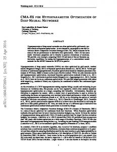
Figure 3: Dendrogram of the considered learning algorithms clustered using unsupervised metalearning based on their classifier output difference. The dashed line represents the cut-point of 0.18 COD value used to create the clusters from which the learning algorithms were selected. diversity between learning algorithms. COD meaTable 1: Set of learning algorithms L used to estimate sures the distance between two learning algorithms p(yi |xi ). as the probability that the learning algorithms make Learning Algorithms different predictions. UML then clusters the learning * Multilayer Perceptron trained with Back algorithms based on their COD scores with hierarchiPropagation (MLP) cal agglomerative clustering. Here, we considered 20 commonly used learning algorithms with their default * Decision Tree (C4.5) hyper-parameters as set in Weka (Hall et al., 2009). * Locally Weighted Learning (LWL) The resulting dendrogram is shown in Figure 3, where * 5-Nearest Neighbors (5-NN) the height of the line connecting two clusters corre- * Nearest Neighbor with generalization (NNge) sponds to the distance (COD value) between them. * Na¨ıve Bayes (NB) A cut-point of 0.18 was chosen and a representative * RIpple DOwn Rule learner (RIDOR) algorithm from each cluster was used to create L as * Random Forest (RandForest) * Repeated Incremental Pruning to Produce Error shown in Table 1. Reduction (RIPPER) In addition to using the entire set L of learning algorithms in the ensemble filter (the L-filter), we also dynamically create the ensemble filter from L using a greedy algorithm. This allows us to find a specific set of learning algorithms that are best for filtering a given data set and learning algorithm combination. Algorithm 1 outlines our approach. The adaptive ensemble filter F is constructed by iteratively adding the learning algorithm g from L that produces the highest cross-validation classification accuracy when g is added to the ensemble filter. Because we are using the probability that an instance will be mis-

classified rather than a binary yes/no, we also use a threshold φ to determine which instances to examine as being detrimental. Instances with a p(yi |xi ) less than φ are discarded from the training set. A constant threshold value for φ is set to filter the instances in runLA(F ) for all iterations. The baseline accuracy for the adaptive approach is the accuracy of the learning algorithm without filtering (line 3). The search stops once adding one of the remaining learning algorithms to the ensemble filter does not 5

4

Algorithm 1 Adaptively identifying detrimental instances. 1: Let F be the set of learning algorithms used for filtering, L be the set of candidate learning algorithms for F , and φ be the threshold such that instances with a p(yi |xi ) less than φ are filtered from the training set. 2: Initialize F to the empty set: F ← {} 3: Initialize current accuracy to the accuracy without filtering: currAcc ← runLA({}). runLA(F ) returns the cross-validation accuracy from a learning algorithm trained on a data set filtered with F . 4: while L 6= {} do 5: bestAcc ← currAcc; bestLA ← null; 6: for all g ∈ L do 7: tempF ← F + g; acc ← runLA(tempF ); 8: if acc > bestAcc then 9: bestAcc ← acc; bestLA ← g; 10: end if 11: end for 12: if bestAcc > currAcc then 13: L ← L − bestLA; F ← F + bestLA; currAcc ← bestAcc; 14: else 15: break; 16: end if 17: end while

Filtering Versus HyperParameter Optimization

In this section, we empirically compare the potential effects of filtering detrimental instances with those of hyper-parameter optimization. When comparing two learning algorithms, statistical significance is determined using the Wilcoxon signed-ranks test (Demˇsar, 2006) with an alpha value of 0.05. In addition to reporting the average classification accuracy, we also report two relative measures–the average percentage of reduction in error and the average percentage of reduction in accuracy, calculated as: %reductionerr = %reductionacc =

g(d)−bl(d) 100−bl(d) , g(d)−bl(d) , bl(d)

if g(d) ≥ bl(d) if g(d) < bl(d)

where bl(d) returns the baseline accuracy on data set d and g(d) returns the accuracy on data set d of the algorithm that we are interested in (i.e., filtering or hyper-parameter optimization). The percent reduction in error captures the fact that increasing the accuracy from 98% to 99% is more difficult than increasing the accuracy from 50% to 51%, which is not expressed in the average accuracy. Likewise, the percent reduction in accuracy captures the relative difference in loss of accuracy for the investigated method. We also show the number of times that g(d) is greater than, equal to, or less than bl(d) (count ). Together, the count, the percent reduction in error, and the percent reduction in accuracy show the potential benefit of the using an algorithm and also the variance of an algorithm. For example, an algorithm has more variance than another if it increases the percent reduction in error but also increases the percent reduction in accuracy compared to an algorithm that may not increase the percent reduction in error as much but also does not increase the percent reduction in accuracy. The average accuracy for each algorithm on a data set is determined using 5 by 10fold cross-validation. Hyper-parameter optimization uses 10 random searches of the hyper-parameter space. Random hyper-parameter selection was chosen based on the work by (Bergstra & Bengio, 2012). The premise of random hyper-parameter optimization is that most

increase accuracy, or all of the learning algorithms in L have been added to the ensemble filter. The adaptive filtering approach overfits the data since the cross validation accuracy is maximized (all detrimental instances are included for evaluation). This allows us to find those instances that are actually detrimental in order to examine the effects that they can have on an induced model. Of course, this is not feasible in practical settings, but provides insight into the potential improvement gained from improving the quality of the training data. 6

machine learning algorithms have very few hyperparameters that considerably affect the final model while most of the other hyper-parameters have little to no effect on the final model. Random search provides a greater variety of the hyper-parameters that considerably affect the model, thus allowing for better selection of these hyper-parameters. Given the same amount of time constraints, random search has been shown to out perform a grid search. For reproducibility, the exact process of hyper-parameter optimization for the learning algorithms is provided in the supplementary material. The accuracy from the hyper-parameters that resulted in the highest crossvalidation accuracy for each data set is reported. For filtering using the ensemble (L-filter) and adaptive filtering, we use thresholds φ of 0.5, 0.3, and 0.1 to identify detrimental instances. The L-filter estimates p(yi |xi ) using all of the learning algorithms in the set L (Table 1). The adaptive filter greedily constructs an ensemble to estimate p(yi |xi ) for a specific data set/learning algorithm combination. The accuracy from the φ that produced the highest accuracy for each data set is reported. To show the effect of filtering detrimental instances and hyper-parameter optimization on an induced model, we examine filtering and hyper-parameter optimization in six commonly used learning algorithms: MLP, C4.5, IBk, NB, Random Forest, and RIPPER. The LWL, NNge, and Ridor learning algorithms are not used for analysis because they do not scale well with the larger data sets–not finishing due to memory overflow or large amounts of running time with many hyper-parameter settings.1 The results comparing the accuracy of the default hyper-parameters set in weka (Hall et al., 2009) with the L-filter and hyper-parameter optimization (HPO) are shown in Table 2. The increases in accuracy that are statistically significant are in bold. Not surprisingly, both the L-filter and hyper-parameter optimization significantly increase the classification accuracy for all of the investigated learning algorithms. The magnitude of the increase in average

Table 2: A comparison of the effects of an ensemble filter and of hyper-parameter optimization on the performance of a learning algorithm. Orig L-filter %rederr %redacc count HPO %rederr %redacc count

MLP 80.74 83.53 16.01 -0.64 44,1,7 83.14 20.24 -2.83 47,0,5

C4.5 80.11 82.57 12.43 -1.23 45,1,6 81.93 12.73 -1.11 39,0,13

IBk 79.03 82.90 18.28 -1.08 44,2,6 82.15 20.02 -0.32 41,2,9

NB 75.68 78.51 14.92 -0.47 42,0,10 79.63 22.77 -0.67 42,1,9

RF 81.59 83.79 14.65 -0.70 38,3,11 82.75 19.81 -2.13 37,2,13

RIP 77.83 81.37 14.96 -0.64 50,0,2 80.04 12.59 -0.48 47,1,4

accuracy is similar for both approaches. However, hyper-parameter optimization shows more variance than filtering as demonstrated by larger percent reduction in error and in a larger percent reduction in accuracy. The L-filter also generally increases the accuracy on more data sets than hyper-parameter optimization. Table 3 compares the hyper-parameter optimized learning algorithms with filtering. L-Forig and LFHPO represent using the L-filter where the learning algorithms in L have default hyper-parameter settings and where the hyper-parameters of the learning algorithms in L have been optimized. Likewise, AHPO and Aorig represent the results from the adaptive filtering algorithm when the ensemble filter is built from L with and without hyper-parameter optimization. Compared with hyper-parameter optimization, the L-filter without hyper-parameter optimization significantly increases the classification accuracy for the C4.5, random forest and RIPPER learning algorithms. However, if the L-filter is composed of hyper-parameter optimized learning algorithms, then the increase in accuracy is significant for all of the considered learning algorithms. The accuracy increases on more data sets for all of the examined learning algorithms when L is composed of hyperparameter optimized learning algorithms. Thus, in combination, hyper-parameter optimization can result in more significant gains in classification accuracy and exhibits less variance.

1 For the data sets on which the learning algorithms did finish, the effects of hyper-parameter optimization and filtering on LWL, NNge, and Ridor are consistent with the other learning algorithms.

7

Table 3: A comparison of the effects of filtering with Table 4: The frequency of selecting a learning algohyper-parameter optimization on the performance of rithm when adaptively constructing a filter set. Each a learning algorithm. row gives the percentage of cases that the learning algorithm was included in the filter set for the learning MLP C4.5 IBk NB RF RIP algorithm in the column. HPO 83.14 81.93 82.15 79.63 82.75 80.04 ALL MLP C4.5 IB5 NB RF RIP L-Forig 83.53 82.57 82.90 78.51 83.79 81.37 %rederr 10.31 9.43 8.26 13.14 12.33 11.98 None 5.36 2.69 2.95 3.08 5.64 5.77 1.60 %redacc -2.11 -2.45 -1.94 -5.65 -1.64 -2.57 MLP 18.33 16.67 15.77 20.00 25.26 23.72 16.36 count 27,3,22 33,4,15 30,2,20 22,2,28 27,1,24 34,1,17 C4.5 17.17 17.82 15.26 22.82 14.49 13.33 20.74 L-FHPO 84.50 83.08 83.83 81.05 85.22 82.85 IB5 12.59 11.92 14.23 1.28 10.00 17.18 16.89 %rederr 11.26 9.24 9.39 8.33 12.34 12.60 LWL 6.12 3.59 3.85 4.36 23.72 3.33 3.59 7.84 5.77 6.54 8.08 5.13 10.26 4.92 %redacc -0.39 -0.13 -0.89 -0.39 -0.06 -0.20 NB count 35,4,13 39,5,8 43,2,7 43,2,7 45,1,6 45,5,2 NNge 19.49 26.67 21.15 21.03 11.15 24.74 23.40 Aorig 88.24 87.39 90.08 81.91 90.17 87.34 RF 21.14 22.95 26.54 23.33 15.77 15.13 24.20 %rederr 37.87 35.22 48.41 22.93 47.02 37.98 Rid 14.69 14.87 16.79 18.33 11.92 16.54 12.77 %redacc -1.41 -0.47 -0.41 -4.69 -1.47 -1.42 RIP 8.89 7.82 7.69 8.85 13.08 7.44 4.39 count 45,0,7 48,2,2 51,0,1 34,0,18 46,0,6 48,0,4 AHPO 85.78 84.45 84.87 82.25 86.57 84.24 random forest, and RIPPER learning algorithms. %rederr 19.23 17.67 16.26 14.66 22.67 21.43 There is no one learning algorithm that is the opti%redacc 0.00 0.00 -0.90 -0.23 0.00 NA mal filter for all learning algorithms and/or data sets. count 50,1,1 47,3,2 49,1,2 49,0,3 50,1,1 50,1,0 Table 4 shows the frequency for which a learning algorithm with default hyper-parameters was selected for filtering by the adaptive filter. The greatest percentage of cases a learning algorithm is selected for filtering for each learning algorithm is in bold. The column “ALL” refers to the average from all of the learning algorithms as the base learner. No instances are filtered in 5.36% of the cases. Thus, filtering to some extent increases the classification accuracy in about 95% of the cases. Furthermore, the random forest, NNge, MLP, and C4.5 learning algorithms are the most commonly chosen algorithms for filtering. However, no one learning algorithm is selected in more than 27% of the cases. The filtering algorithm that is most appropriate is dependent on the data set and the learning algorithm. Previously, S´ aez et al. (2013) examined when filtering is most beneficial for the nearest neighbor classifier. They found that the efficacy of noise filtering is dependent on the characteristics of the data set and provided a rule set to determine when filtering will be most beneficial. Future work includes better understanding the efficacy of noise filtering for each learning algorithm and determining which filtering approach to use for a given

The adaptive filter also significantly improves classification accuracy over hyper-parameter optimization and provides a greater increase in accuracy than the L-filter with hyper-parameter optimization. The results from the adaptive filters show the potential gain in filtering if a filtering algorithm could more accurately identify detrimental instances for each data set and learning algorithm combination. With and without hyper-parameter optimization, the adaptive filter results in significant gains in generalization accuracy for each learning algorithm. These results show the impact of choosing an appropriate subset of the training data and provide motivation for improving filtering algorithms. Building an adaptive filter from the set of learning algorithms without hyper-parameter optimization provides higher average classification accuracy but also exhibits more variance. However, the adaptive filter composed of hyper-parameter optimized learning algorithms increases the accuracy on more data sets than the adaptive filter composed of learning algorithms with their default hyper-parameters for the MLP, na¨ıve Bayes, 8

data set.

5

seeks to clean or correct instances that are noisy or possibly corrupted (Kubica & Moore, 2003). However, this could artificially corrupt valid instances. Weighting, on the other hand, weights suspected detrimental instances rather than discarding them (Rebbapragada & Brodley, 2007; Smith & Martinez, 2014b). Weighting the instances allows for an instance to be considered on a continuum of detrimentality rather than making a binary decision of an instance’s detrimentality. These approaches have the advantage that data is not discarded which is especially beneficial when data is scarce. Much of the previous work has artificially inserted noise and/or corrupted instances into the initial data set to determine how well an approach would work in the presence of noisy or mislabeled instances. In some cases, a given approach only has a significant impact when there are large degrees of artificial noise. We show that correctly labeled, non-noisy instances can also be detrimental for inducing a model of the data and that properly handling them can result in significant gains in classification accuracy. Thus, in contrast to much previous work, we did not artificially corrupt a data set to create detrimental instances. Rather, we sought to identify the detrimental instances that are already contained in a data set. The grid search and manual search are the most common types of hyper-parameter optimization techniques in machine learning. A combination of the two approaches are commonly used (Larochelle et al., 2007). Bayesian optimization has also been used to search the hyper-parameter space (Snoek et al., 2012; Hutter et al., 2011) as an alternative approach. Further, Bergstra & Bengio (2012) proposed to use a random search of the hyper-parameter space as discussed previously.

Related Work

To our knowledge, this is the first work that examines both filtering and hyper-parameter optimization in handling detrimental instances and compares their effects. Our work was motivated in part by Smith et al. (2013) who examined the existence of and characterization of instances that are hard to classify correctly. They found that a significant number of instances are hard to classify correctly and that the hardness of each instance is dependent on its relationship with the other instances in the training set as well as the learning algorithm used to induce a model of the data. Thus, there is a need for improving the way detrimental instances are handled during training as they affect the classification of the other instances in the data set. Other previous work has examined improving the quality of the training data and hyper-parameter optimization in isolation. Fr´enay & Verleysen (2014) provide a survey of the current approaches for dealing with label noise in classification problems which often take the approach of improving the quality of the data. Improving the quality of the training data has typically fallen into three approaches: filtering, cleaning, and instance weighting. Each technique within an approach differs in how detrimental instances are identified. A common technique for filtering removes instances from a data set that are misclassified by a learning algorithm (Tomek, 1976) or an ensemble of learning algorithms (Brodley & Friedl, 1999). Removing the training instances that are suspected to be noise and/or outliers prior to training has the advantage that they do not influence the induced model and generally increase classification accuracy (Smith & Martinez, 2011). Training on a subset of the training data has also been observed to increase accuracy in active learning (Schohn & Cohn, 2000). A negative side-effect of filtering is that beneficial instances can also be discarded and produce a worse model than if all of the training data had been used (Smith & Martinez, 2014a). Rather than discarding the instances from a training set, one approach

6

Conclusions

In this paper we compared the potential benefits of filtering with hyper-parameter optimization both mathematically and empirically. Mathematically, hyper-parameter optimization may reduce the effects of detrimental instances on an induced model but the detrimental instances are still considered in the 9

learning process. Filtering, on the other hand, fully removes the detrimental instances–completely eliminating the effects of the detrimental instances on the induced model. Empirically, we estimated the potential benefits of each method by maximizing the 10-fold crossvalidation accuracy of each data set. For the adaptive filter, we also chose a set of learning algorithms for an ensemble filter by maximizing the 10fold cross-validation accuracy. Both filtering and hyper-parameter optimization significantly increase the classification accuracy for all of the considered learning algorithms. On average, a learning algorithm increases in classification accuracy from 79.15% to 87.52% by removing the detrimental instances on the observed data sets using the adaptive filter. On the other hand, hyper-parameter optimization only increases the average classification accuracy to 81.61%. Filtering with hyper-parameter optimized learning algorithms produces more stable results (i.e. consistent increases in classification accuracy and low decreases in classification accuracy) than filtering or hyper-parameter optimization in isolation. One of the reasons that instance subset selection is overlooked is due to the fact that there is a large computational requirement to observe the relationship of an instance on the other instances in a data set. As such, determining which instances to filter is non-trivial. We hope that the results presented in this paper will provide motivation for furthering the work in improving the quality of the training data.

References

Demˇsar, Janez. Statistical comparisons of classifiers over multiple data sets. Journal of Machine Learning Research, 7:1–30, 2006. Elman, Jeffery L. Learning and development in neural networks: The importance of starting small. Cognition, 48:71–99, 1993. Fr´enay, Benoit and Verleysen, Michel. Classification in the presence of label noise: a survey. IEEE Transactions on Neural Networks and Learning Systems, pp. in press, 25 pages, 2014. Hall, Mark, Frank, Eibe, Holmes, Geoffrey, Pfahringer, Bernhard, Reutemann, Peter, and Witten, Ian H. The weka data mining software: an update. SIGKDD Explorations Newsletter, 11 (1):10–18, 2009. Hutter, Frank, Hoos, Holger H., and Leyton-Brown, Kevin. Sequential model-based optimization for general algorithm configuration. In Proceedings of the International Learning and Intelligent Optimization Conference, pp. 507–523, 2011. Kubica, Jeremy and Moore, Andrew. Probabilistic noise identification and data cleaning. In Proceedings of the 3rd IEEE International Conference on Data Mining, pp. 131–138, 2003. Larochelle, Hugo, Erhan, Dumitru, Courville, Aaron, Bergstra, James, and Bengio, Yoshua. An empirical evaluation of deep architectures on problems with many factors of variation. In Proceedings of the 24th International Conference on Machine Learning, pp. 473–480, 2007.

Bergstra, James and Bengio, Yoshua. Random search Lee, Jun and Giraud-Carrier, Christophe. A metfor hyper-parameter optimization. Journal of Maric for unsupervised metalearning. Intelligent Data chine Learning Research, 13:281–305, 2012. Analysis, 15(6):827–841, 2011. Brodley, Carla E. and Friedl, Mark A. Identifying Nettleton, David F., Orriols-Puig, Albert, and Formislabeled training data. Journal of Artificial Innells, Albert. A study of the effect of different telligence Research, 11:131–167, 1999. types of noise on the precision of supervised learning techniques. Artificial Intelligence Review, 33 Collobert, Ronan, Sinz, Fabian, Weston, Jason, and (4):275–306, 2010. Bottou, L´eon. Trading convexity for scalability. In Proceedings of the 23rd International Conference Peterson, Adam H. and Martinez, Tony R. Estimating the potential for combining learning models. on Machine learning, pp. 201–208, 2006. 10

In Proceedings of the ICML Workshop on MetaLearning, pp. 68–75, 2005.

Wolpert, David H. The lack of a priori distinctions between learning algorithms. Neural Computation, 8(7):1341–1390, 1996.

Rebbapragada, Umaa and Brodley, Carla E. Class noise mitigation through instance weighting. In Zhu, Xingquan and Wu, Xindong. Class noise vs. attribute noise: a quantitative study of their imProceedings of the 18th European Conference on pacts. Artificial Intelligence Review, 22:177–210, Machine Learning, pp. 708–715, 2007. November 2004. S´ aez, Jos´e A., Luengo, Juli´ an, and Herrera, Francisco. Predicting noise filtering efficacy with data complexity measures for nearest neighbor classification. Pattern Recognition, 46(1):355–364, 2013. Schohn, Greg and Cohn, David. Less is more: Active learning with support vector machines. In Proceedings of the 17th International Conference on Machine Learning, pp. 839–846, 2000. Smith, Michael R. and Martinez, Tony. Improving classification accuracy by identifying and removing instances that should be misclassified. In Proceedings of the IEEE International Joint Conference on Neural Networks, pp. 2690–2697, 2011. Smith, Michael R. and Martinez, Tony. An extensive evaluation of filtering misclassified instances in supervised classification tasks. In submission, 2014a. URL http://arxiv.org/abs/1312.3970. Smith, Michael R. and Martinez, Tony. Becoming more robust to label noise with classifier diversity. In Submission, 2014b. URL http://arxiv.org/abs/1403.1893. Smith, Michael R., Martinez, Tony, and GiraudCarrier, Christophe. An instance level analysis of data complexity. Machine Learning, pp. in press, 32 pages, 2013. doi: 10.1007/s10994-013-5422-z. Snoek, Jasper, Larochelle, Hugo, and Adams, Ryan. Practical bayesian optimization of machine learning algorithms. In Advances in Neural Information Processing Systems 25, pp. 2960–2968. 2012. Tomek, Ivan. An experiment with the edited nearestneighbor rule. IEEE Transactions on Systems, Man, and Cybernetics, 6:448–452, 1976. 11