The Proceeding.pdf - School of Computer Science

ISSN 1858 -1633 Proceeding of Annual International Conference

Information and Communication Technology Seminar Volume 1, Number 1, August 2005 Executive Board Rector of ITS Dean of Information Technology Faculty (FTIF) ITS Head of Informatics Department FTIF ITS Editorial Board Achmad Benny Mutiara Gunadharma University, Indonesia

Marco J Patrick V-SAT Company, Portugal

Agus Zainal Sepuluh Nopember Institute of Technology, Indonesia

Mauridhi Hery Purnomo Sepuluh Nopember Institute of Technology, Indonesia

Akira Asano Hiroshima University, Japan

Muchammad Husni Sepuluh Nopember Institute of Technology, Indonesia

Archi Delphinanto Eindhoven University of Technology, The Netherlands

Nanik Suciati Sepuluh Nopember Institute of Technology, Indonesia

Arif Djunaidy Sepuluh Nopember Institute of Technology, Indonesia

Riyanarto Sarno Sepuluh Nopember Institute of Technology, Indonesia

Daniel Siahaan Sepuluh Nopember Institute of Technology, Indonesia

Rothkrantz Delft University of Technology, Indonesia

Handayani Tjandrasa Sepuluh Nopember Institute of Technology

Retantyo Wardoyo Gajah Mada University, Indonesia

Happy Tobing Cendrawasih University, Indonesia

Siska Fitriana Delft University of Technology, The Netherlands

Hideto Ikeda Ritsumeikan University, Japan

Supeno Djanali Sepuluh Nopember Institute of Technology, Indonesia

Johny Moningka Indonesia University, Indonesia

Zainal Hasibuan Indonesia University, Indonesia

Joko Lianto Sepuluh Nopember Institute of Technology, Indonesia

Yudhi Purwananto Sepuluh Nopember Institute of Technology, Indonesia

Kridanto Surendro Bndung Institute of Technology, Indonesia

i

ISSN 1858 -1633

Editor-in-Chief Umi Laili Yuhana Sepuluh Nopember Institute of Technology, Indonesia

Contact Address Informatics Department FTIF, ITS Gedung Teknik Informatika ITS, Jl. Raya ITS, Sukolilo Surabaya 60111, INDONESIA Telp. (031) 5939214 Fax (031) 5913804 Homepage: http://if.its.ac.id/icts email:[email protected]

ii

ISSN 1858 -1633

PREFACE This proceedings contain sorted papers from Information and Communication Technology Seminar (ICTS) 2005. ICTS 2005 is the first annual international event from Informatics Department, Faculty of Information Technology, ITS. This event is a forum for computer science, information and communication technology community for discussing and exchanging the information and knowledge in their areas of interest. It aims to promote activities in research, development, and application on computer science, information and communication technology. This year, the seminar is held to celebrate the 20th Anniversary of Informatics Department, Faculty of Information Technology, ITS. There are 41 papers accepted and finally 36 papers are fit and proper to be presented. The topics of those papers are: (1) Artificial Intelligence (2) Image Processing (3) Computing (4) Computer Network and Security (5) Software Engineering and (6) Mobile Computing. We would like to thank to the keynote speakers, the authors, the participants, and all parties for the success of ICTS 2005. Editorial Team

iii

ISSN 1858 -1633

Proceeding of Annual International Conference

Information and Communication Technology Seminar Volume 1, Number 1, August 2005 Table of Content Mathematical Morphology And Its Applications ...................................................................1-9 Akira Asano Molecular Dynamics Simulation On A Metallic Glass-System: Non-Ergodicity Parameter ...............................................................................................................................10-16 Achmad Benny Mutiara Tomographic Imaging Using Infra Red Sensors.................................................................17-19 Dr. Sallehuddin Ibrahim and Md. Amri Md. Yunus Mammographic Density Classification Using Multiresolution Histogram Technique ...20-23 Izzati Muhimmah, Erika R.E. Denton, and Reyer Zwiggelaar Ann Soft Sensor To Predict Quality Of Product Based On Temperature Or Flow Rate Correlation..............................................................................................................................24-28 Totok R. Biyanto Application Of Soft Classification Techniques For Forest Cover Mapping ....................29-36 Arief Wijaya Managing Internet Bandwidth: Experience In Faculty Of Industrial Technology, Islamic University Of Indonesia.........................................................................................................37-40 Mukhammad Andri Setiawan Mue: Multi User Uml Editor.................................................................................................41-45 Suhadi Lili, Sutarsa, and Siti Rochhimah Designing Secure Communication Protocol For Smart Card System, Study Case: E-Purse Application..............................................................................................................................46-48 Daniel Siahaan, and I Made Agus Fuzzy Logics Incorporated To Extended Weighted-Tree Similarity Algorithm For Agent Matching In Virtual Market .................................................................................................49-54 Sholeh Hadi Setyawan and Riyanarto Sarno Shape Matching Using Thin-Plate Splines Incorporated To Extended Weighted-Tree Similarity Algorithm For Agent Matching In Virtual Market..........................................55-61 Budianto and Riyanarto Sarno Text-To-Video Text To Facial Animation Video Convertion ............................................62-67 Hamdani Winoto, Hadi Suwastio, and Iwan Iwut T.

iv

ISSN 1858 -1633

Share-It: A UPnP Application For Content Sharing..........................................................68-71 Daniel Siahaan Modified Bayesian Optimization Algorithm For Nurse Scheduling .................................72-75 I N. Sutapa, I. H. Sahputra, and V. M. Kuswanto Politeness In Phoning By Using Wap And Web ..................................................................76-80 Amaliah Bilqis, and Husni Muhammad Impelementation Of Hierarchy Color Image Segmentation For Content Based Image Retrieval System.....................................................................................................................81-85 Nanik Suciati and Shanti Dewi Decision Support System For Stock Investment On Mobile Device.................................86-90 Ivan Satria and Dedi Trisnawarman Fuzzy Logic Approach To Quantify Preference Type Based On Myers Briggs Type Indicator (MBTI)....................................................................................................................91-93 Hindriyanto Dwi Purnomo, Srie Yulianto Joko Prasetyo Security Concern Refactoring.............................................................................................94-100 Putu Ashintya Widhiartha, and Katsuhisa Maruyama A Parallel Road Traffic Simulator Core ..........................................................................101-104 Dwi Handoko, Wahju Sediono, and Made Gunawan C/I Performance Comparison Of An Adaptive And Switched Beam In The Gsm Systems Employing Smart Antenna................................................................................................105-110 Tito Yuwono, Mahamod Ismail, and Zuraidah bt Zainuddin Identification Of Solvent Vapors Using Neural Network Coupled Sio2 Resonator Array.................................................................................................................111-114 Muhammad Rivai, Ami Suwandi JS , and Mauridhi Hery Purnomo Comfortable Dialog For Object Detection .......................................................................115-122 Rahmadi Kurnia A Social Informatics Overview Of E-Government Implementation: Its Social Economics And Restructuring Impact ................................................................................................123-129 Irwan Sembiring and Krismiyati Agent Based Programming For Computer Network Monitoring .................................130-134 Adang Suhendra Computer Assisted Diagnosis System Using Morphology Watershed For Breast Carcinoma Tumor..................................................................................................................................135-139 Sri Yulianto and Hindriyanto

v

ISSN 1858 -1633

Evaluation Of Information Distribution Algorithms Of A Mobile Agent-Based DemandOriented Information Service System.............................................................................140-144 I. Ahmed and M J. Sadiq Online Mobile Tracking On Geographics Information System Using Pocket Pc........145-150 M. Endi Nugroho and Riyanarto Sarno A Simple Queuing System To Model The Traffic Flow At The Toll-Gate: Preliminary Results .................................................................................................................................151-153 Wahju Sediono, Dwi Handoko Multimodal-Eliza Perceives And Responds To Emotion ...............................................154-158 S. Fitrianie and L.J.M. Rothkrantz Motor Dc Position Control Based On Moving Speed Controlled By Set Point Changing Using Fuzzy Logics Control System ................................................................................159-166 Andino Maseleno, Fajar Hayyin, Hendra, Rahmawati Lestari, Slamet Fardyanto, and Yuddy Krisna Sudirman A Variable-Centered Intelligent Rule System .................................................................167-174 Irfan Subakti Multiple Null Values Estimating In Generating Weighted Fuzzy Rules Using Genetic Simulated Annealing..........................................................................................................175-180 Irfan Subakti Genetic Simulated Annealing For Null Values Estimating In Generating Weighted Fuzzy Rules From Relational Database Systems ......................................................................181-188 Irfan Subakti Image Thresholding By Measuring The Fuzzy Sets Similarity .....................................189-194 Agus Zainal Arifin and Akira Asano Development Of Scheduler For Linux Virtual Server In Ipv6 Platform Using Round Robin Adaptive Algorithm, Study Case: Web Server ...............................................................195-198 Royyana Muslim Ijtihadie and Febriliyan Samopa

vi

Information and Communication Technology Seminar, Vol. 1 No. 1, August 2005

1

MATHEMATICAL MORPHOLOGY AND ITS APPLICATIONS Akira Asano Division of Mathematical and Information Sciences, Faculty of Integrated Arts and Sciences, Hiroshima University Kagamiyama 1-7-1, Higashi-Hiroshima, Hiroshima 739-8521, JAPAN email: [email protected]

ABSTRACT This invited talk presents the concept of mathematical morphology, which is a mathematical framework of quantitative image manipulations. The basic operations of mathematical morphology, the relationship to image processing filters, the idea of size distribution and its application to texture analysis are explained.

1. INTRODUCTION Mathematical morphology treats an effect on an image as an effect on the shape and size of objects contained in the image. Mathematical morphology is a mathematical system to handle such effects quantitatively based on set operations [1–5].The word stem “morpho-” originates in a Greek word meaning “shape,” and it appears in the word “morphing,” which is a technique of modifying an image into another image smoothly. The founders of mathematical morphology, G. Mathéron and J. Serra, were researchers of l ´ Ecole Nationale Supérieure des Mines de Paris in France, and had an idea of mathematical morphology as a method of evaluating geometrical characteristics of minerals in ores [6]. Mathéron is also the founder of the random closed set theory, which is a fundamental theory of treating random shapes, and kriging, which is a statistical method of estimating a spatial distribution of mineral deposits from trial diggings. Mathematical morphology has relationships to these theories and has been developed as a theoretical framework of treating spatial shapes and sizes of objects. The International Symposium on Mathematical Morphology (ISMM), which is the topical international symposium focusing on mathematical morphology only, has been organized almost every two years, and its seventh symposium was held in April 2005 in Paris as a cerebration of 40 years anniversary of mathematical morphology [7]. The paper explains the framework of mathematical morphology, especially opening, which is the fundamental operation of describing operations on shapes and sizes of objects quantitatively, in Sec. 2. Section 3. proves “filter theorem,” which guarantees that all practical image processing filters can be constructed by combinations of morphological operations. Examples of expressing median filters and average filters by combinations of morphological operations are also shown in this section. Section 4.

explains granulometry, which is a method of measuring the distribution of sizes of objects in an image, and shows an application to texture analysis by the author.

2. BASIC OPERATIONS OF MATHEMATICAL MORPHOLOGY The fundamental operation of mathematical morphology is “opening,” which discriminates and extracts object shapes with respect to the size of objects. We explain opening on binary images at first, and basic operations to describe opening.

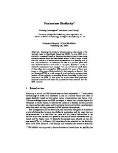
2.1 Opening In the context of mathematical morphology, an object in a binary image is regarded as a set of vectors corresponding to the points composing the object. In the case of usual digital images, a binary image is expressed as a set of white pixels or pixels of value one. Another image set expressing an effect to the above image set is considered, and called structuring element. The structuring element corresponds to the window of an image processing filter, and is considered to be much smaller than the target image to be processed. Let the target image set be X, and the structuring element be B. Opening of X by B has a property as follows: where Bz indicates the translation of B by z, defined as follows: This property indicates that the opening of X with respect to B indicates the locus of B itself sweeping all the interior of X, and removes smaller white regions than the structuring element, as illustrated in Fig. 1. Since opening eliminates smaller structures and smaller bright peaks than the structuring element, it has a quantitative smoothing ability.

ISSN 1858-1633 @2005 ICTS


2

Fig. 1. Effect of opening.

2.2.

Fig. 2. opening composed of fundamental operations.

Fundamental Operations Mathematical Morphology

of

Although the property of opening in E. (1) is intuitively understandable, this is not a pixelwise operation. Thus opening is defined by a composition of simpler pixelwise operations. In order to define opening, Minkowski set subtraction and addition are defined as the fundamental operations of mathematical morphology.

Minkowski set subtraction has the following property: It follows from x ∈ Xb that x − b ∈ X. Thus the definition of Minkowski set subtraction in Eq. (3) can be rewritten to the following pixelwise operation: The reflection of B, denoted ˇB , is defined as follows:

Using the above expressions, Minkowski set subtraction is expressed as follows: Since we get from the definition of reflection in Eq. (6) that

, it follows

. We get the that relationship in Eq. (7) by substituting it into Eq. (5).This relationship indicates that

It indicates that is composed by pasting a copy of B at every point within X. Using the above operations, erosion and dilation of X with respect to B are defined as and . respectively. We get from Eq. (7) that It indicates that is the locus of the origin of B when B sweeps all the interior of X. The opening XB is then defined using the above fundamental operations as follows: The above definition of opening is illustrated in Fig. 2. A black dot indicates a pixel composing an image object in this figure. As shown in the above, the erosion of X by B is the locus of the origin of B when B sweeps all the inside of X. Thus the erosion in the first step of opening produces every point where a copy of B included in X can be located. The Minkowski addition in the second step locates a copy of B at every point within . Thus the opening of X with respect to B indicates the locus of B itself sweeping all the interior of X, as described at the beginning of this section. In other words, the opening removes regions of X which are too small to include a copy of B and preserves the others. The counterpart of opening is called closing, defined as follows: The closing of X with respect to B is equivalent to the opening of the background, and removes smaller spots than the structuring element within image objects. This is because the following relationship between opening and closing holds:

is the

when sweeps all the locus of the origin of interior of X. For Minkowski set addition, it follows that

where Xc indicate the complement of X and defined as The relationship of Eq. (13) is called duality of opening and closing1. 1

Thus we get

There is another notation system which denotes opening as X ◦ B and closing as X • B.

ISSN 1858-1633 @2005 ICTS

Mathematical Morphology and Its Application – Akira Asano

Figure 3 summarizes the illustration of the effects of basic morphological operations2.

Fig. 3. Effects of erosion, dilation, opening, and closing

3

where w(g) is the support of g. These equations indicate that the logical AND and OR operations in the definition for binary images are replaced with the infimum and supremum operations (equivalent to minimum and maximum in the case of digital images), respectively. Expanding the idea, mathematical morphological operations can be defined for sets where the infimum and supremum among the elements are defined in some sense. For example, morphological operations for color images cannot be defined straightforwardly from the above classical definitions, since a color pixel value is defined by a vector and the infimum and supremum are not trivially defined. The operations can be defined if the infimum and supremum among colors are defined [8, 9]. Such set is called lattice, and mathematical morphology is generally defined as operations on a lattice [10].

3. MATHEMATICAL MORPHOLOGY AND IMAGE PROCESSING FILTER 3.1. Morphological filter

Fig. 4. Umbra. The spatial axis x is illustrated one-dimensional for simplicity.

2.3. In the Case of Gray Scale Images In the case of gray scale image, an image object is defined by the umbra set. If the pixel value distribution of an image object is denoted as f(x), where is a pixel position, its umbra U[f(x)] is defined as follows: Consequently, when we assume a “solid” whose support is the same as a gray scale image object and whose height at each pixel position is the same as the pixel value at this position, the umbra is equivalent to this solid and the whole volume below this solid within the support, as illustrated in Fig. 4. A gray scale structuring element is also defined in the same manner. Let f(x) be the gray scale pixel value at pixel position x and g(y) be that of the structuring element. Erosion of f by g is defined for the umbrae similarly to the binary case, and reduced to the following operation [4, 5]: Dilation is also reduced to 2 There is another definition of morphological operations which denotes the erosion in the text as X _ B and call the Minkowski set addition in the text “dilation.” The erosion and dilation are not dual in this definition,

Image processing filter is generally an operation at each pixel by applying a calculation to the pixel and the pixels in its neighborhood and replacing the pixel value with the result of calculation, for the purposes of noise removal, etc. Morphological filter in broader sense is restricted to translation-invariant and increasing one. An operation Ψ on a set (image) X is translation-invariant if In other words, it indicates that the effect of the operation is invariant wherever the operation is applied. An operation Ψ is increasing if In other words, the relationship of inclusion is preserved before and after applying the operation. Let us consider a noise removing filter for example; Since noise objects in an image should be removed wherever it is located, the translationinvariance is naturally required for noise removing filters. An increasing operation can express an operation that removes smaller objects and preserves larger objects, but cannot express an operation that removes larger and preserves smaller. Noise objects are, however, usually smaller than meaningful objects. Thus it is also natural to consider increasing operations only3. Morphological filter in narrower sense is all translation-invariant, increasing, and idempotent operations. The filter Ψ is idempotent if 3

Edge detecting filter is not increasing, since it removes all parts of objects

ISSN 1858-1633 @2005 ICTS


4

Consequently, iterative operations of Ψ is equivalent to one operation of Ψ . The opening and closing are the most basic morphological filters in narrower sense.

and

is satisfied if

,

we get

. By denoting

by

, we get Consequently,

. there exists

element

3.2. Filter theorem The filter theorem states that all morphological filters (in broader sense) can be expressed by OR of erosions and AND of dilations. It guarantees that almost all practical filters can be expressed by morphological operations, i. e. mathematical morphology is really a fundamental operation set of image object manipulations. Let Ψ(X) be a filter on the image X. The theorem states that there exists for all Ψ(X) a set family Ker[Ψ] satisfying the following.

a

structuring

such

that

, i. e. any pixel in Ψ(X) can be included in

by using a

certain structuring element

. Thus

From the above discussion, it holds that

3.3. Morphological expressions of median filter and average filter It also states that there exists for all Ψ(X) a set family Ker[Ψ] satisfying the following.

Here the set family Ker[Ψ] is called kernel of filter Ψ, defined as follows: where “0” indicates the origin of X. The proof of the filter theorem in Eq. (20) is presented in the following. A more general proof is found in Chap. 4 of [10]. Let us consider an arbitrary vector (pixel) for .

a

From

structuring the

element

definition

of

. Consequently, Since Ψ is increasing, the relationship B ⊆ X−h is invariant by filter Ψ. Thus we get translation-invariant,

. we

Since

Ψ

is get translating

by

. From the above discussion, for all structuring element

.

an arbitrary vector translation-invariant,

Thus

The filter theorem guarantees that all translationinvariant increasing filters can be constructed by morphological operations. However, the kernel is generally redundant and each practical filter is often expressed by morphological operations with fewer numbers of structuring elements. In this subsection, morphological expressions of median filter and average filter are shown with examples. These filters are usually applied to gray scale images, morphological operations and logical operations are reduced to minimum and maximum operations. Details of the proof are found in [11, 12]. 3.3.1. Median filter: The median filter whose window size is n pixel is expressed as follows: the minimum of maximum ( or the maximum of minimum) in every possible subwindow of [n/2 + 1] pixels in the window. The operations deriving the maximum and minimum in each subwindow at every pixel are the set addition and set subtraction using the subwindow as the structuring element, respectively. Since the maximum and minimum operations are extensions of logical OR and AND operations based on fuzzy logic, respectively, the median filter is expressed by the combination of morphological and logical operations, as shown in Figs. 5 and 6.

. Let us consider . Since Ψ is . Thus we get

.

Since ,

ISSN 1858-1633 @2005 ICTS


5

Fig. 7. Average expressed by the maximum and minimum.

4. GRANULOMETRY AND TEXTURE ANALYSIS

Fig. 5. Subwindows of [n/2 + 1] pixels.

3.3.2. Average filter: The simplest average filter operation, that is, the average of two pixel values x and y, is expressed by the minimum and the supremum, as follows:

Texture is an image composed by repetitive appearance of small structures, for example surfaces of textiles, microscopic images of ores, etc. Texture analysis is a fundamental application of mathematical morphology, since it was developed for the analysis of minerals in ores. In this section, the concept of size in the sense of mathematical morphology and the idea of granulometry for measuring granularity of image objects are explained. An example of texture analysis applying granulometry by the author is also presented.

4.1. Granulometry and size distribution or

as shown in Fig. 7.

Fig. 6. Median expressed by the maximum and minimum.

Opening of image X with respect to structuring element B means residue of X obtained by removing smaller structures than B. It indicates that opening works as a filter to distinguish object structures by their sizes. Let 2B, 3B, . . . , be homothetic magnifications of the basic structuring element B. We then perform opening of X with respect to the homothetic structuring elements, and obtain the image sequence XB, X2B, X3B, . . . . In this sequence, XB is obtained by removing the regions smaller than B, X2B is obtained by removing the regions smaller than X2B, X3B is obtained by removing the regions smaller than 3B, . . . . If B is convex, it holds that X XB X2B X3B . . . . The size of rB is defined as r, and this sequence of opening is called granulometry [10]. We then calculate the ratio of the area (for binary case) or the sum of pixel values (for gray scale case) of XrB to that of the original X at each r. The area of an image is defined by the area occupied by an image object, i. e. the number of pixels composing an image object in the case of discrete images. The function from a size r to the corresponding ratio is monotonically decreasing, and unity when the size is zero. This function is called size distribution function. The size distribution function of size r indicates the area ratio of the regions whose sizes are greater than or equal to r.

ISSN 1858-1633 @2005 ICTS

6


Fig. 8. Granulometry and size density function

The r-times magnification of B, denoted rB, is usually defined in the context of mathematical morphology as follows:

where {0} denotes a single dot at the origin. Let us consider a differentiation of the size distribution function. In the case of discrete sizes, it is equivalent to the area differences of the image pairs corresponding to adjacent sizes in XB, X2B, X3B, .... For example, the area difference between X2B and X3B corresponds to the part included inX2B but excluded fromX3B, that is, the part whose size is exactly 2. The sequence of the areas corresponding to each size exactly, derived as the above, is called pattern spectrum [13], and the sequence of the areas relative to the area of the original object is called size density function [14]. An example of granulometry and size density function is illustrated in Fig. 8. Size distribution function and size density function have similar properties to probability distribution function and probability density function, respectively, so that such names are given to these functions. Similarly to probability distributions, the average and the variance of size of objects in an image can be considered. Higher moments of a size distribution can be also defined, which are called granulometric moments, and image objects can be characterized using these moments [14–16].

4.2. Application to texture analysis As described in Sec. 2., morphological opening is a regeneration of an image by arranging the structuring element, and removes smaller white regions in binary case or smaller regions composed of brighter pixels than its neighborhood in gray scale case than the

structuring element. Thus opening is effective for eliminating noisy pixels that are brighter than its neighborhood. Since opening generates the resultant image by an arrangement of the structuring element, the hape and pixel value distribution of the structuring element directly appear in the resultant image. It causes artifacts if the shape and pixel value distribution are not related to the original image. This artifact can be suppressed by using a structuring element resembling the shape and pixel value distribution contained in the original image. Such structuring element cannot be defined generally, but can be estimated for texture images, since texture is composed an arrangement of small objects appearing repetitively in the texture. We explain in this subsection a method of developing the optimal artifact-free opening for noise removal in texture images [17]. This method estimates the structuring element which resembles small objects appearing repetitively in the target texture. This is achieved based on Primitive, Grain, and Point Configuration (PGPC) texture model, which we have proposed to describe a texture, and an optimization method with respect to the size distribution function. The optimal opening of suppressing the artifacts is achieved by using the estimated structuring element. In the case of noise removal, the primitive cannot be estimated by the target image itself, since the original uncorrupted image corresponding to the target image is unknown. This problem is similar to that of the image processing by learning, which estimates the optimal filter parameters by giving an example of corrupted image and its ideal output to a learning mechanism [18–20]. In the case of texture image, however, if a sample uncorrupted part of the texture similar to the target corrupted image is available, the primitive can be estimated from this sample, since the sample and the target image are different realization but have common textural characteristics. 4.2.1. PGPC texture model and estimation of the optimal structuring element: The PGPC texture model regards a texture as an image composed by a regular or irregular arrangement of objects that are much smaller than the size of image and resemble each other. The objects arranged in a texture are called grains, and the grains are regarded to be derived from one or a few typical objects called primitives. We assume here that the grains are derived from one primitive by homothetic magnification.We also assume that the primitive is expressed by a structuring element B, and let X be the target texture image. In this case, XrB is regarded as the texture image composed by the arrangement of rB only. It follows that rB − (r + 1)B indicates the region included in the arrangement of rB but not included in that of (r+1)B. Consequently, XrB −X(r+1)B is the region where r-size grains are arranged if X is expressed by employing an

ISSN 1858-1633 @2005 ICTS


arrangement of grains which are preferably large magnifications of the primitive. The sequence X − XB, XB − X2B, . . . , XrB − X(r+1)B, . . . , is the decomposition of the target texture to the arrangement of the grains of each size. Since the sequence can be derived by using any structuring element, it is necessary to estimate the appropriate primitive that is a really typical representative of the grains. We employ an idea that the structuring element yielding the simplest grain arrangement is the best estimate of the primitive, similarly to the principle of minimum description length (MDL). The simple arrangement locates a few number of large magnifications for the expression of a large part of the texture image, contrarily to the arrangement of a large number of small-size magnifications. We derive the estimate by finding the structuring element minimizing the integral of 1 − F(r), where F(r) is the size distribution function with respect to size r. The function 1 − F(r) is 0 for r = 0 and monotonically increasing, and 1 for the maximum size required to compose the texture by the magnification of this size. Consequently, if the integral of 1−F(r) is minimized as illustrated in Fig. 9, the sizes of employed magnifications concentrate to relatively large sizes, and the structuring element in this case expresses the texture using the largest possible magnifications. We regard this structuring element as the estimate of primitive. We estimate the gray scale structuring element in two steps: the shape of structuring element is estimated by the above method in the first step, and the gray scale value at each pixel in the primitive estimated in the first step is then estimated. However, if the above method is applied to the gray scale estimation, the estimate often has a small number of high-value pixel and other pixels whose values are almost zero. This is because the umbra of any object can be composed by arranging the umbra of one-pixel structuring element, as illustrated in Fig. 10. This is absolutely not a desired estimate. Thus we modify the above method, and minimize 1 − F(1), i. e. the residual area of XB instead of the above method. In this case, the composition by this structuring element and its magnification is the most admissible when the residual area is the minimum, since the residual region cannot be composed of even the smallest magnification. The exploration of the structuring element can be performed by the simulated annealing, which iterates a modification of the structuring element and find the best estimate minimizing the evaluation function described in the above [21].

7

Fig. 9. Function 1 − F(r). Size r is actually discrete for digital images.(a)Function and its integral. (b) Minimization of the integral.

Fig. 10. Any object can be composed by arranging one-pixel structuring element.

4.2.2. Experimental results: Figures 11 and 12 show the example experimental results of noise removal using the estimated primitives as the structuring elements. All images contains 64×64 8-bit gray scale pixels. In each example, the gray scale primitive shown in (b) is estimated for the example image (a). Each small square in (b) corresponds to one pixel in the primitive, and the shape is expressed by the arrangement of white squares. The primitive is explored from connected figures of nine pixels within 5 × 5-pixel square. The gray scale value is explored by setting the initial pixel value to 50 and modifying the value in the range of 0 to 100. The opening using the primitive (b) as the structuring element is performed on the corrupted image (c). This image is generated by adding a uniformly distributed random value, which is in the range between 0 and 255, to 1000 randomly selected pixels of an image extracted from an image which is a different realization of the same texture as (a). Opening eliminates brighter peaks of small extent, so that this kind of noise is employed for this experiment.

ISSN 1858-1633 @2005 ICTS

8


The result using the estimate primitive is shown in (d), that using the flat structuring element whose shape is the same as (b) is shown in (e), and that using the 3 × 3-pixel square flat structuring element is shown in (f). The “MSE” attached to each resultant image is defined as the sum of pixelwise difference between each image and the original uncorrupted image of (c), which is not shown here, divided by the number of pixels in the image.

In these examples, the assumptions that the grains are derived from one primitive by homothetic magnification and the primitive is expressed by one structuring element are not exactly satisfied. However, the results indicate that our method is applicable to these cases practically.

5. CONCLUSIONS This invited talk has explained the fundamental concept of mathematical morphology, the filter theorem and the relationship to image processing filters, and the concept of size distribution and its application to texture analysis, which is one of the author’s research topics. The importance of mathematical morphology is that it gives a “mathematical” framework based on set operations to operations on shapes and sizes of image objects. Mathematical morphology has its origin in the research of minerals; If the researchers of mathematical morphology had concentrated to practical problems only and had not made efforts of mathematical formalization, mathematical morphology could not have been extended to general image processing or spatial statistics. It suggests that researches on any topic considering general frameworks is always important.

Fig. 11. Experimental results (1).

The results (d) show high effectiveness of our method in noise removal and detail preservation. The results using the square structuring element contain artifacts since the square shape appears directly in the results, and the results using the binary primitives yield regions of unnaturally uniform pixel values. The comparison of (d) and (e) indicates that the optimization of binary structuring elements is insufficient and the grayscale optimization is necessary.

Fig. 12. Experimental results (2).

Acknowledgements The author would like to thank Dr. Daniel Siahaan, the Organizing Committee Chairman, and all the Committee members, for this opportunity of the invited talk in ICTS2005.

REFERENCES [1] J. Serra, Image analysis and mathematical morphology, Academic Press, 1982. ISBN012-637242-X [2] J. Serra, ed., Image analysis and mathematical morphology Volume 2, Technical advances, Academic Press, 1988. ISBN0-12-637241-1 [3] P. Soille, Morphological Image Analysis, 2nd Ed., Springer, 2003. [4] P. Maragos, Tutorial on advances in morphological image processing and analysis, Optical Engineering, 26, 1987, 623–632. [5] R. M. Haralick, S. R. Sternberg, and X. Zhuang, Image Analysis Using Mathematical Morphology, IEEE Trans. Pattern Anal. Machine Intell., PAMI-9, 1987, 532–550. [6] G. Matheron, J. Serra, The birth of mathematical morphology, Proc. 6th International Symposium on Mathematical Morphology, 1–16, CSIRO Publishing 2002. ISBN0-643-06804-X [7] International Symposium on Mathematical Morphology, 40 years on (http://ismm05.esiee.fr).

ISSN 1858-1633 @2005 ICTS


[8] M. L. Corner and E. J. Delp, Morphological operations for color image processing, Journal of Electronic Imaging, 8(3), 1999, 279–289. [9] G. Louverdis, M. I. Vardavoulia, I. Andreadis, and Ph. Tsalides, A new approach to morphological color image processing, Pattern Recognition, 35, 2002, 1733–1741. [10] H. J. A. M. Heijmans, Morphological Image Operators, Academic Press (1994). ISBN0-12014599-5 [11] P. Maragos and R. W. Schafer, Morphological Filters- Part I, Their Set-Theorectic Analysis and Relations to Linear Shift-Invariant Filters, IEEE Trans. Acoust., Speech, Signal Processing, ASSP-35(8), 1987, 1153–1169 . [12] P. Maragos and R. W. Schafer, Morphological Filters- Part II, Their Relations to Median, Order-Statistic, and Stack Filters, IEEE Trans. Acoust., Speech, Signal Processing, ASSP35(8), 1987, 1170–1184 . [13] P. Maragos, Pattern spectrum and multiscale shape representation, IEEE Trans. Pattern Anal. Machine Intell., 11, 1989, 701–716. [14] E. R. Dougherty, J. T. Newell, and J. B. Pelz, Morphological texturebased maximumllikelihood pixel classification based on local granulometric moments, Pattern Recognition, 25, 1992, 1181–1198. [15] F. Sand and E. R. Dougherty, Asymptotic granulometric mixing theorem, morphological estimation of sizing parameters and mixture

9

[16] [17]

[18]

[19]

[20]

[21]

proportions, Pattern Recognition, 31, 1998, 53–61. F. Sand and E. R. Dougherty, Robustness of granulometric moments, Pattern Recognition, 32, 1999, 1657–1665. A. Asano, Y. Kobayashi, C. Muraki, and M. Muneyasu, Optimization of gray scale morphological opening for noise removal in texture images, Proc. 47th IEEE International Midwest Symposium on Circuits and Systems, 1, 2004, 313–316. A. Asano, T. Yamashita, and S. Yokozeki, Learning optimization of morphological filters with grayscale structuring elements, Optical Engineering, 35(8), 1986, 2203–2213. N. R. Harvey and S. Marshall, The use of genetic algorithms in morphological filter design, Signal Processing, Image Communication, 8, 1996, 55–71. N. S. T. Hirata, E. R. Dougherty, and J. Barrera, Iterative Design of Morphological Binary Image Operators, Optical Engineering, 39(12), 2000, 3106–3123. A. Asano, T. Ohkubo, M. Muneyasu, and T. Hinamoto, Primitive and Point Configuration texture model and primitive estimation using mathematical morphology, Proc. 13th Scandinavian Conf. on Image Analysis, Göteborg, Sweden; Springer LNCS 2749, 2003, 178–185.

ISSN 1858-1633 @2005 ICTS


10

MOLECULAR DYNAMICS SIMULATION ON A METALLIC GLASS-SYSTEM: NON-ERGODICITY PARAMETER Achmad Benny Mutiara Dept. of Informatics Engineering, Faculty of Industrial Technology, Gunadarma University Jl.Margonda Raya No.100, Depok 16424, West-Java Indonesia E-mail: [email protected]

ABSTRACT At the present paper we have computed nonergodicity paramater from Molecular Dynamics (MD) Simulation data after the mode-coupling theory (MCT) for a glass transition. MCT of dense liquids marks the dynamic glass-transition through a critical temperature Tc that is reflected in the temperaturedependence of various physical quantities. Here, molecular dynamics simulations data of a model adapted to Ni0.2Zr0.8 are analyzed to deduce Tc from the temperature-dependence of corresponding quantities and to check the consistency of the statements. Analyzed is the diffusion coefficients. The resulting values agree well with the critical temperature of the non-vanisihing non-ergodicity parameter determined from the structure factors in the asymptoticsolution of the mode-coupling theory with memorykernels in “One-Loop” approximation. Keywords: Glass Transition, Molecular Dynamics Simulation, MCT

1. INTRODUCTION The transition from a liquid to an amorphous solid that sometimes occurs upon cooling remains one of the largely unresolved problems of statistical physics [1,2]. At the experimental level, the so-called glass transition is generally associated with a sharp increase in the characteristic relaxation times of the system, and a concomitant departure of laboratory measurements from equilibrium. At the theoretical level, it has been proposed that the transition from a liquid to a glassy state is triggered by an underlying thermodynamic (equilibrium) transition [3]; in that view, an “ideal” glass transition is believed to occur at the so-called Kauzmann temperature, TK. At TK, it is proposed that only one minimum-energy basin of attraction is accessible to the system. One of the first arguments of this type is due to Gibbs and diMarzio [4], but more recent studies using replica methods have yielded evidence in support of such a transition in Lennard-Jones glass formers [3,5,6]. These observations have been called into question by experimental data and recent results of simulations of polydisperse hard-core disks, which have failed to detect any evidence of a thermodynamic transition up to extremely high packing fractions [7]. Oneof the questions that arises is therefore whether the discrepancies between the reported simulated behavior

of hard-disk and soft-sphere systems is due to fundamental differences in the models, or whether they are a consequence of inappropriate sampling at low temperatures and high densities. Different, alternative theoretical considerations have attempted to establish a connection between glass transition phenomena and the rapid increase in relaxation times that arises in the vicinity of a theoretical critical temperature (the so-called “modecoupling” temperature, Tc), thereby giving rise to a “kinetic” or “dynamic” transition [8]. In recent years, both viewpoints have received some support from molecular simulations. Many of these simulations have been conducted in the context of models introduced by Stillinger andWeber and by Kob and Andersen [9]; such models have been employed in a number of studies that have helped shape our current views about the glass transition [5,10–14]. In the full MCT, the remainders of the transition and the value of Tc have to be evaluated, e.g., from the approach of the undercooled melt towards the idealized arrested state, either by analyzing the time and temperature dependence in the β-regime of the structural fluctuation dynamics [15–17] or by evaluating the temperature dependence of the socalled gm-parameter [18,19]. There are further posibilities to estimates Tc, e.g., from the temperature dependence of the diffusion coefficients or the relaxation time of the final α-decay in the melt, as these quantities for T > Tc display a critical behaviour |T − Tc|±γ. However, only crude estimates of Tc can be obtained from these quantities, since near Tc the critical behaviour is masked by the effects of transversale currents and thermally activated matter transport, as mentioned above. On the other hand, as emphasized and applied in [20–22], the value of Tc predicted by the idealized MCT can be calculated once the partial structure factors of the system and their temperature dependence are sufficiently well known. Besides temperature and particle concentration, the partial structure factors are the only significant quantities which enter the equations of the so-called nonergodicity parameters of the system. The latter vanish identically for temperatures above Tc and their calculation thus allows a rather precise determination of the critical temperature predicted by the idealized theory. At this stage it is tempting to consider how well the estimates of Tc from different approaches fit

ISSN 1858-1633 @2005 ICTS

Molecular Dynamics Simulation on A Metallic Glass-System: Non-Ergodicity Parameter – Achmad Benny Mutiara together and whether the Tc estimate from the nonergodicity parameters of the idealized MCT compares to the values from the full MCT. Regarding this, we here investigate a molecular dynamics (MD) simulation model adapted to the glass-forming Ni0.2Zr0.8 transition metal system. The NixZr1−xsystem is well studied by experiments [23,24] and by MD-simulations [25–29], as it is a rather interesting system whose components are important constituents of a number of multi-component ’massive’ metallic glasses. In the present contribution we consider, in particular, the x = 0.2 compositions and concentrate on the determination of Tc from evaluating and analyzing the non-ergodicity parameter and the diffusion coefficients. In the literature, similar comparison of Tc estimates already exist [20–22] for two systems. The studies come, however, to rather different conclusions. From Mdsimulations for a soft spheres model, Barrat et.al. [20] find an agreement between the different Tc estimates within about 15%. On the other hand, for a binary Lennard-Jones system, Nauroth and Kob [22] get from their MD simulations a significant deviation between the Tc estimates by about a factor of 2. Regarding this, the present investigation is aimed at clarifying the situation for at least one of the important metallic glass systems. Our paper is organized as follows: In Section II, we present the model and give some details of the computations. Section III gives a brief discussion of some aspects of the mode coupling theory as used here. Results of our MD-simulations and their analysis are then presented and discussed in Section IV.

2. SIMULATIONS The present simulations are carried out as state-oftheart isothermal-isobaric (N, T, p) calculations. The Newtonian equations of N = 648 atoms (130 Ni and 518 Zr) are numerically integrated by a fifth order predictorcorrector algorithm with time step ∆t = 2.5x10−15s in a cubic volume with periodic boundary conditions and variable box length L. With regard to the electron theoretical description of the interatomic potentials in transition metal alloys by Hausleitner and Hafner [30], we model the interatomic couplings as in [26] by a volume dependent electron-gas term Evol(V ) and pair potentials φ(r) adapted to the equilibrium distance, depth, width, and zero of the HausleitnerHafner potentials [30] for Ni0.2Zr0.8 [31]. For this model simulations were started through heating a starting configuration up to 2000 K which leads to a homogeneous liquid state. The system then is cooled continuously to various annealing temperatures with cooling rate −∂tT = 1.5x1012 K/s. Afterwards the obtained configurations at various annealing temperatures (here 1500-800 K) are relaxed by carrying out additional isothermal annealing run at the selected temperature. Finally the time evolution of

11

these relaxed configurations is modelled and analyzed. More details of the simulations are given in [31].

3. THEORY In this section we provide some basic formulae that permit calculation of Tc and the non-ergodicity parameters fij(q) for our system. A more detailed presentation may be found in Refs. [20–22,32,33]. The central object of the MCT are the partial intermediate scattering functions which are defined for a binary system by [34]

where

is a Fourier component of the microscopic density of species i. The diagonal terms α = β are denoted as the incoherent intermediate scattering function

The normalized partial- and intermediate scattering functions are given by

incoherent

where the Sij(q) = Fij(q, t = 0) are the partial static structure factors. The basic equations of the MCT are the set of nonlinear matrix integrodifferential equations given by

where F is the 2×2 matrix consisting of the partial intermediate scattering functions Fij(q, t), and the frequency matrix Ω2 is given by

S(q) denotes the 2 × 2 matrix of the partial structure factors Sij(q), xi = Ni/N and mi means the atomic mass of the species i. The MCT for the idealized glass transition predicts [8] that the memory kern M can be expressed at long times by

ISSN 1858-1633 @2005 ICTS

12


where ρ = N/V is the particle density and the vertex Viαβ(q, k) is given by

and the matrix of the direct correlation function is defined by

The equation of motion for Fs i (q; t) has a similar form as eq.(6), but the memory function for the incoherent intermediate scattering function is given by:

This iterative procedure, indeed, has two type of solutions, nontrivial ones with f (q) > 0 and trivial solutions f (q) = 0. The incoherent non-ergodicity parameter fs i (q) can be evaluated by the following iterative procedure:

As indicated by eq.(20), computation of the incoherent non-ergodicity parameter fs i (q) demands that the coherent non-ergodicity parameters are determined in advance.

4. RESULTS AND DISCUSSIONS 4.1 Partial structure factors and intermediate scattering functions In order to characterize the long time behaviour of the intermediate scattering function, the nonergodicity parameters f (q) are introduced as

These parameters are the solution of eqs. (6)-(10) at long times. The meaning of these parameters is the following: if fij(q) = 0, then the system is in a liquid state with density fluctuation correlations decaying at long times. If fij(q) > 0, the system is in an arrested, nonergodic state, where density fluctuation correlations are stable for all times. In order to compute fij(q), one can use the following iterative procedure [22]:

where the matrix A(q), B(q),C(q), D(q), N(q) is given by

First we show the results of our simulations concerning the static properties of the system in terms of the partial structure factors Sij(q) and partial correlation functions gij(r). To compute the partial structure factors Sij(q) for a binary system we use the following definition [35]

where

are the partial pair correlation functions. The MD simulations yield a periodic repetition of the atomic distributions with periodicity length L. Truncation of the Fourier integral in Eq.(21) leads to an oscillatory behavior of the partial structure factors at small q. In order to reduce the effects of this truncation, we compute from Eq.(22) the partial pair correlation functions for distance r up to Rc = 3=2L. For numerical evaluation of eq.(21), a Gaussian type damping term is included

ISSN 1858-1633 @2005 ICTS

Molecular Dynamics Simulation on A Metallic Glass-System: Non-Ergodicity Parameter – Achmad Benny Mutiara

13

FIG. 2. Comparison between our MD-simulations and experimental results [23] of the total Faber-Ziman structure factor SFZ tot (q) and the partial Faber-Ziman structur factors aij(q) for Ni0:2Zr0:8.

FIG. 1. Partial structure factors at T = 1400 K, 1300 K, 1200 K, 1100 K, 1000 K, 900 K and 800 K (from top to bottom); a) Ni-Nipart, the curves are vertically shifted by 0.05 relative to each other; b) Ni-Zr-part, the curves are vertically shifted by 0.1 relative to each other; and c) Zr-Zr-part, the curves are vertically shifted by 0.5 relative to each other.

with R = Rc=3. Fig.1 shows the partial structure factors Sij(q) versus q for all temperatures investigated. The figure indicates that the shape of Sij(q) depends weakly on temperature only and that, in particular, the positions of the first maximum and the first minimum in Sij(q) are more or less temperature independent. In order to compare our calculated structure factors with experimental ones, we have determined the Faber- Ziman partial structure factors aij(q) [37]

and the Faber-Ziman total structure factor SFZ tot (q) [36]. For a binary system with coherent scattering length bi of species i the following relationship holds:

In the evaluation of aij(q), we applied the same algorithm as for Sij(q). By using aij(q) and with aids of the experimental data of the average scattering

ISSN 1858-1633 @2005 ICTS

14


length b one can compute the total structure factor. Here we take bi from the experimental data of Kuschke [23]. b for natural Ni is 1.03 (10¡12 cm) and for Zr 0.716 (10¡12 cm). Fig.2 compares the results of our simulations with the experimental results by Kuschke [23] for the same alloy system at 1000 K. There is a good agreement between the experimental and the simulations results which demonstrates that our model is able to reproduce the steric relations of the considered system and the chemical order, as far is visible in the partial structure factors.

4.2 Non-ergodicity parameters The non-ergodicity parameters are defined over Eq.(13) as a non-vanishing asymptotic solution of the MCT-eq.(6). Phenomenologically, they can be estimated by creating a master curve from the intermediate scattering functions with fixed scattering vector q at different temperatures. The master curves are obtained by plotting the scattering functions ©(q; t) as function of the normalized time t=¿®. Fig. 3 presents the estimated q-dependent nonergodicity parameters from the coherent scattering functions of Ni and Zr, Fig. 4 those from the incoherent scattering functions. In Fig. 3 and 4 are also included the deduced Kohlrausch-Williams-Watts amplitudes A(q) from the master curves and from the intermediate scattering functions at T=1100 K. (The further fitparameters can be found in [31].) In order to compute the non-ergodicity parameters fij(q) analytically, we followed for our binary system the self-consistent method as formulated by Nauroth and Kob [22] and as sketched in Section III.A. Input data for our iterative determination of fij(q) = Fij(q;1) are the temperature dependent partial structure factors Sij(q) from the previous subsection. The iteration is started by arbitrarily setting FNi¡Ni(q;1)(0) = 0:5SNi¡Ni(q), FZr¡Zr(q;1)(0) = 0:5SZr¡Zr(q), FNi¡Zr(q;1)(0) = 0.

FIG. 3. Non-ergodicity parameter fcij for the coherent intermediate scattering functions as solutions of eqs. (7) and (8)(solid line), KWW-parameter A(q) of the master curves (diamond), Von Schweidler-parameter fc(q) of the master curves (square), and KWW-parameter A(q) for ©ij(q) at 1100 K (triangle up); a) Ni-Nipart and b) Zr-Zr-part.

ISSN 1858-1633 @2005 ICTS

Molecular Dynamics Simulation on A Metallic Glass-System: Non-Ergodicity Parameter – Achmad Benny Mutiara

15

1102 K . Fig. 4 presents our results for so calculated fs ci(q). Like Fig. 3 for the coherent non-ergodicity parameters, Fig. 4 demonstrates for the fs ci(q) that they agree well with the estimates from the incoherent scattering functions master curve and, in particular, with the deduced Kohlrausch-Williams-Watts amplitudes A(q) at 1100 K.

4.3 Diffusion-coeffient From the simulated atomic motions in the computer experiments, the diffusion coefficients of the Ni and Zr species can be determined as the slope of the atomic mean square displacements in the asymptotic long-time limit

FIG. 4. The same as fig.3 but for the incoherent intermediate scattering function; a) Ni-part and b) Zr-part.

For T > 1200 K we always obtain the trivial solution fij(q) = 0 while at T = 1100 K and below we get stable non-vanishing fij(q) > 0. The stability of the non-vanishing solutions was tested for more than 3000 iteration steps. From this results we expect that Tc for our system lies between 1100 and 1200 K. To estimate Tc more precisely, we interpolated Sij(q) from our MD data for temperatures between 1100 and 1200 K by use of the algorithm of Press et.al. [39]. We observe that at T = 1102 K a non-trivial solution of fij(q) can be found, but not at T = 1105 K and above. It means that the critical temperature Tc for our system is around 1102 K. The non-trivial solutions fij(q) for this temperature shall be denoted the critical nonergodicity parameters fcij(q). They are included in Fig. 3. As can be seen from Fig. 3, the absolute values and the q-dependence of the calculated fcij(q) agree rather well with the estimates from the scattering functions master curve and, in particular, with the deduced Kohlrausch-Williams-Watts amplitudes A(q) at 1100 K. By use of the critical non-ergodicity parameters fcij(q), the computational procedure was run to determine the critical non-ergodicity parameters fs ci(q) for the incoherent scattering functions at T =

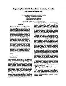
FIG. 5. Diffusion coefficients Di as a function of 1000=T . Symbols are MD results for Ni (square) and Zr (diamond); the full line are a power-law approximation for Ni and for Zr. resp..

Fig. 5 shows the thus calculated diffusion coefficients of our Ni0:2Zr0:8 model for the temperature range between 800 and 2000 K. At temperatures above approximately 1250 K, the diffusion coefficients for both species run parallel with temperature in the Arrhenius plot, indicating a fixed ratio DNi=DZr ¼ 2:5 in this temperature regime. At lower temperatures, the Zr atoms have a lower mobility than the Ni atoms, yielding around 900 K a value of about 10 for DNi=DZr. That means, here the Ni atoms carry out a rather rapid motion within a relative immobile Zr matrix. According to the MCT, above Tc the diffusion coefficients follow a critical power law with non-universal exponent ° [9,38]. In order to estimate Tc from this relationship, we have adapted the critical power law by a least mean squares fit to the

ISSN 1858-1633 @2005 ICTS

16


simulated diffusion data for 1050 K and above. The results of the fit are included in Fig. 5 by dashed lines. According to this fit, the system has a critical temperature of 950 K. The parameters ° turn out as 1.8 for the Ni subsystem and 2.0 for the Zr system.

5. CONCLUSION The results of our MD-simulations show that our system behave so as predicted by MCT in the sense that the diffusion coefficients follow the critical power law. After analizing this coefficient we found that the system has critical temperature of 950 K. diffusionprocesses. Our analysis of the ergodic region ( T > Tc ) and of the non-ergodic region ( T < Tc ) lead to Tcestimations which agree each other within 10 %. These Tc-estimations are also in acceptable compliance with the Tc-estimation from the dynamic phenomenons. Within the scope of the precision of our analysis, the critical temperatur Tc of our system is about 1000 K.

REFERENCES [1]

W. Götze and M. Sperl, J. Phys.: Condens. Matter 16, 4807 (2004); W. Götze and M. Sperl, Phys.Rev.Lett. 92, 105701 (2004) [2] P. G. Debenedetti and F.H. Stillinger, Nature 410(6825), 259 (2001). [3] M. Mezard and G. Parisi, Phys.Rev.Lett. 82(4), 747 (1999). [4] J.H. Gibbs and E. A. DiMarzio, J.Chem.Phys. 28(3), 373 (1958). [5] B.Colluzi, G.Parisi, and P.Verrochio, Phys.Rev.Lett.84(2), 306(2000). [6] T. S. Grigera and G. Parisi, Phys. Rev. E 63, 045102(R) (2001). [7] L. Santen and W. Krauth, Nature 405(6786), 550 (2000). [8] W. Götze and L. Sjögren, Rep. Prog. Phys. 55(3), 241 (1992) [9] W. Kob und H.C. Andersen, Phys. Rev. E 51(5), 4626 (1995). [10] S. Sastry, P. G. Debendetti and F. H. Stillinger, Nature 393(6685), 554 (1998). [11] F. Sciortino, W. Kob, and P. Tartaglia, Phys. Rev. Lett. 83(16), 3214 (1999). [12] C. Donati, S. C. Glotzer, P. H. Poole, W. Kob, and S. J. Plimpton, Phys.Rev. E 60(3), 3107 (1999) [13] B. Colluzi, G. Parisi, and P. Verrochio, Phys. Rev. Lett. 112(6), 2933 (2000). [14] R. Yamamoto and W. Kob, Phys.Rev. E 61(5), 5473 (2000) [15] T. Gleim and W. Kob, Eur. Phys. J. B 13, 83 (2000).

[16] A. Meyer, R. Busch, and H. Schober, Phys. Rev. Lett. 83, 5027 (1999); A. Meyer, J. Wuttke, W. Petry, O.G. Randl, and H. Schober, Phys. Rev. Lett. 80, 4454 (1998). [17] H.Z. Cummins, J. Phys.Cond.Mat. 11, A95 (1999). [18] H. Teichler, Phys. Rev. Lett. 76, 62(1996). [19] H. Teichler, Phys. Rev. E 53, 4287 (1996). [20] J.L. Barrat und A. Latz, J. Phys. Cond. Matt. 2, 4289 (1990). [21] M. Fuchs, Thesis, TU-Muenchen (1993); M. Fuchs und A. Latz, Physica A 201, 1 (1993). [22] M. Nauroth and W. Kob, Phys. Rev. E 55, 657 (1997). [23] M. Kuschke, Thesis, Universität Stuttgart (1991). [24] Yan Yu, W.B. Muir und Z. Altounian, Phys. Rev. B 50, 9098 (1994). [25] B. Böddekker, Thesis, Universität Göttingen (1999); Böddekker and H. Teichler, Phys. Rev. E 59, 1948 (1999) [26] H. Teichler, phys. stat. sol. (b) 172, 325 (1992) [27] H. Teichler, in: Defect and Diffusion Forum 143-147, 717 (1997) [28] H. Teichler, in: Simulationstechniken in der Materialwissenschaft, edited by P. Klimanek and M. Seefeldt (TU Bergakadamie, Freiberg, 1999). [29] H. Teichler, Phys. Rev. B 59, 8473 (1999). [30] Ch. Hausleitner and Hafner, Phys. Rev. B 45, 128 (1992). [31] A.B. Mutiara, Thesis, Universität Göttingen (2000). [32] W. Götze, Z. Phys. B 60, 195 (1985). [33] J. Bosse und J.S. Thakur, Phys. Rev. Lett. 59, 998(1987). [34] B. Bernu, J.-P. Hansen, G. Pastore, and Y. Hiwatari, Phys. Rev A 36, 4891 (1987); ibid. 38, 454 (1988). [35] J.P. Hansen and I.R. McDonald, Theory of Simple Liquids, 2nd Ed. ( Academic Press, London, 1986). [36] T.E. Faber und J.M. Ziman, Phil. Mag. 11, 153 (1965). [37] Y. Waseda, The Structure of Non-Crystalline Materials, (McGraw-Hill, New York, 1980). [38] J.-P. Hansen and S. Yip, Transp. Theory Stat. Phys. 24, 1149 (1995). [39] W.H. Press, B.P. Flannery, S.A. Teukolsky und W.T. Vetterling, Numerical Recipes, 2nd.Edition (University Press, Cambrigde, New York, 1992)

ISSN 1858-1633 @2005 ICTS


17

TOMOGRAPHIC IMAGING USING INFRA RED SENSORS Sallehuddin Ibrahim & Md. Amri Md. Yunus Department of Control and Instrumentation Engineering Faculty of Electrical Engineering, Universiti Teknologi Malaysia 81310 UTM Skudai, Johor, Malaysia [email protected]

ABSTRAK This paper is concerned with the development of a tomographic imaging system in order to measure a two-phase flow involving solid particles flowing in air. The general principle underlying a tomography system is to attach a number of non-intrusive transducers in plane formation to the vessel to be investigated and recover from those sensors an image of the corresponding cross section through the vessel. The method made use of infra red sensors. The sensors were configured as a combination of two orthogonal and two rectilinear light projection system. It has the ability to accurately visualize concentration profiles in a pipeline. The imaging is carried out online without invading the fluids. The system used a combination of two orthogonal and two rectilinear infra-red projections. The sensors were installed around a vertical transparent flow pipe. Several results are presented in this paper showing the capability of the system to visualize the concentration profiles of solids flowing in air. Keywords: Infra red, imaging, tomography, sensor.

1. INTRODUCTION Flow imaging is gaining importance in process industries. As such suitable systems must be developed for this purpose. Flow measurements belong to the most difficult ones because the medium being measured can occur in various physical states, which complicate the measuring procedure. They are, namely, temperature, density, viscosity, pressure, multi-component media (liquid-gas, solid-gas), the type of flow, etc. The choice of the method is further directed by specific requirements for the flowmeter, e.g. the measuring range, minimum loss of pressure, the shortest possible recovery section, a sensor without moving parts, continuous operation of the sensor, etc. Tomography methods have been developed rapidly for visualizing two-phase flow of various industrial processes, e.g. gas/oil flows in oil pipelines [1], gas/solid flows in pneumatic conveyors [2], and separation/mixing processes in chemical vessels [3]. Infra red tomography involves the measurement of light attenuation detected by various infra red sensors installed around a flow pipe, and the reconstruction of cross-sectional images using the measured data and a suitable algorithm.

Tomography began to be considered seriously as it can be used to directly analyze the internal characteristics of process flow so that resources will be utilized in a more efficient manner and in order to meet the demand and regulations for product quality. The use of tomography to analyze the flow regime began in the late 1980s. Besides, concern about environmental pollution enhanced the need to find alternative methods of reducing industrial emission and waste. In those applications, the system must be robust and does not disturb the flow in pipelines. It should be able to operate in aggressive and fast moving fluids. This is where tomography can play an important role as it can unravel the complexities of flow without invading it. Tomography can be combined with the characteristics of infra red sensors to explore the internal characteristics of a process flow. Infra red tomography is conceptually straightforward and inexpensive. It has a dynamic response and can be more portable compared to other types of radiationbased tomography system. The image reconstruction by an infra red tomography system should be directly associated to visual images observed in transparent sections of the pipelines. It has other advantages such as negligible response time relative to process variations, high resolution, and immunity to electrical noise and interference. This paper will explain how such a system can be designed and constructed to measure the distribution of solids in air flowing in a pipeline.

2. IMAGE RECONSTRUCTION The projection of infra red beam from the emitter towards the detector can be illustrated mathematically in Figure 1. The coordinate system can be utilized to describe line integrals and projections. The object of interest is represented by a two-dimensional function f(x,y) and each line integral is represented by the (Ø, x’) parameters. Line AB can be expressed as x cosφ + y sinφ = x' (1) where

⎡ x'⎤ ⎡ cos φ ⎢ y '⎥ = ⎢− sin φ ⎣ ⎦ ⎣

sin φ ⎤ ⎡ x ⎤ cos φ ⎥⎦ ⎢⎣ y ⎥⎦

(2) which resulted in the following line integral

ISSN 1858-1633 @2005 ICTS


18

∫ f ( x, y)dx

pφ ( x' ) =

(3)

(φ , x ') line

Using a delta function, this can be rewritten as

pφ ( x ' ) =

M −1

⎡ N −1

M =0

N =0

∑ ⎢⎣ ∑

⎤ f ( x , y ) ∂ ( x cos φ + y sin φ ) ∆ x ⎥ ∆ y ⎦

(4) where N = total number of horizontal cells/pixel M = total number of vertical cells/pixel The algorithm for reconstruction is performed by approximating the density at a point by summing all the ray sum of the ray through the point. This has been termed the discrete back projection method and can be formulated mathematically as

1 fˆ ( x, y ) = M

⎡

⎤

M −1 N −1

∑ ⎢⎣∑ p(φ , x')∂( x cos φ + y sin φ − x' )∆x'⎥⎦∆φ

m = 0 n =0

(5) (5) Projections

x’

pφ ( x1 ' )

A y’

y

of the flow. The flow pipe has an external diameter of 80 mm and an internal diameter of 78mm. Since the infra red sensors are the critical part, the selection of infra red transmitters and receivers are considered carefully. The sensors should be arranged such that they cover the whole pipe. In tomography, the more number of sensors used means higher resolution is achieved. Another set of sensors were constructed 100mm downstream to measure velocity using the cross-correlation method. The sensors used must be of high performance, compact, require minimum maintenance or calibration and be intrinsically safe. For this purpose, the emitter SFH 4510 and detector SFH 2500 was chosen due to its low cost and fast switching time. The infra red emitters and detectors are arranged in pairs. They are linked to the measurement section through optical fibers. Each receiver circuit consists of a photodiode, pre-amplification, amplification and a filter. The receiver circuits are connected to a data acquisition card manufactured by Keithley. The card is of the type DAS-1800. Light generated by the emitters passed to flow pipe and is attenuated if it hits an object. The light reaches the receiver and is then converted by a photodiode into current by the receiving circuit. The signal is processed by a signal conditioning circuit. Data then entered the data acquisition system and is converted into a digital form prior to entering the computer. A linear back projection algorithm was developed which processed the digitized signal and displayed the concentration profile of the solids flowing in air. The algorithm is programmed in the Visual C++ language which is a powerful tool for such purpose.

X’

φ°

f ( x, y)

x B

Figure 1. Infra red path from emitter to detector

3. SYSTEM DESIGN The measurement system composed of four subsystems: (1) sensor, (2) signal conditioning, (3) data acquisition system, and (4) image reconstruction and display. Figure 2 depicts the measurement section around the flow pipe which contains 64 pairs of infra red sensors configured in a combination of orthogonal and rectilinear projection. A similar number of sensors are installed downstream. The output of the downstream sensors should be a replica of the output from the upstream sensors but experienced a time delay. Both signals can be cross-correlated to obtain the velocity

Figure 2. Tomographic measurement section

The solid particles consisting of plastic beads were dropped onto a gravity flow rig shown in Figure 3. The rig costing about RM100,000 was supplied by Optosensor. The beads were filled into a hopper and a rotary valve controls the amount of beads flowing into the rig. Thus user can set various flow rates. The measurement section was installed around the flow rig.

ISSN 1858-1633 @2005 ICTS

Tomographic Imaging Using Infra Red Sensors – Sallehuddin Ibrahim & Md. Amri Md. Yunus

19

Hopper

Pipeline Figure 5(c). Concentration profile at a flow rate of 71 g/s

4. RESULT Various experiments were carried out using various algorithms and at various flow rates. The regression graph is shown in Figure 4. The concentration profiles at various flow rates are shown in Figures 5(a) to 5(c). Figure 4 shows that the output from upstream sensors have similar values to that of the downstream sensors and the sensors output is proportional to the mass flow rates. Figures 5(a) to 5(c) show that the infra red tomographic system is able to locate the position of the beads inside the flow pipe. At higher flow rates, the flow rig released more plastic beads that at lower flow rates. As such more pixels are occupied in Figures 5(b) and 5(c) compared to Figure 5(a).

Tank Figure 3. Gravity fvlow rig

5. CONCLUSION Figure 4. The regression line of sensors output versus measured mass flow rates

A tomographic imaging system using infra red sensors has been designed. The system is capable of producing tomographic images for two-phase flow. The spatial resolution and measurement accuracy can be enhanced by adding more sensors. However, there must be a compromise between the spatial resolution, accuracy and real-time capability of the system. The system has the potential of being applied in various process industries.

REFERENCES Figure 5(a). Concentration profile at a flow rate of 27 g/s

[1] S. Ibrahim and M. A. Md. Yunus , Preliminary Result for Infrared Tomography, Elektrika., 6 (1), 2004, 1 – 4. [2] S. McKee, T. Dyakowski, R.A. Williams, T.A. Bell and T. Allen,Solids flow imaging and attrition studies in a pneumatic conveyor, Powder Technology, 82, 1995, 105 – 113. [3] F. Dickin, Electrical resistance tomography for process applications, Meas. Sci. Technol., 7(3), 1996, 247-260.

Figure 5(b). Concentration profile at a flow rate of 49 g/s

ISSN 1858-1633 @2005 ICTS


20

MAMMOGRAPHIC DENSITY CLASSIFICATION USING MULTIRESOLUTION HISTOGRAM TECHNIQUE Izzati Muhimmah1, Erika R.E. Denton2, Reyer Zwiggelaar3 Jurusan Teknik Informatika, FTI, Universitas Islam Indonesia, Yogyakarta 55584, Indonesia, 2 Department of Breast Imaging, Norwich and Norfolk University Hospital, Norwich NR2 7UY, UK, 3 Department of Computer Science, University of Wales Aberystwyth, Aberystwyth SY23 1LB, UK 1

ABSTRACT Mammographic density is known to be an important indicator of breast cancer risk. Some quantitative estimation approaches have been developed and among of them based on histogram measurement. We implemented multi-resolution histogram technique to classify density of mammographic images. The results showed an agreement of 38,33% (78:33% when minor classification was allowed) compare to an expert radiologist rating using SCC given in EPIC database. This agreement is lower than the existing methods, and some limitations are discussed. Keywords : density classification, mammographic, breast cancer, medical imaging, multi-resolution histogram

1. INTRODUCTION Mammographic images are 2D projections of the x-ray attenuation properties of the 3D breast tissues along the path of the x-rays. The connective and epitheal tissues attenuate harder than fatty tissues, which would 'burn' more silver grains on mammograpic films. This phenomenon can be interpreted that brighter area on the mammograms films represents glandular tissues, whereas the dark area represent fatty tissues. Mammographic parenchymal patterns provide a strong indicator of the risk of developing breast cancer. The first attempt to relate them was introduced by Wolfe[11]. This method subdivides breast parenchymal pattern into four classes, which are N1, P1, P2, and DY. The classification solely based on visual assessment whether or not there are prominent duct patterns and their severities as seen by mammography, in other word, this approach gives considerable heterogeneity in risk estimates reported. The study of Boyd et. al [1] gives an alternative approach to estimate breast cancer risk for given mammograms. It is based on proportion of breast occupied by densities (i.e, relative areas) to subdivide mammogram into six class categories (SCC), which the highest class indicates the highest risk, see Figure 1. This classification method can be seen as a quantitative approach to estimate breast cancer risk, so as can be implemented for computer-assisted methods. As be mentioned earlier, mammographic densities

correlates with brighter appearance on mammograms. In image analysis point of view, it can be seen as correspondence between mammographic densities and image intensities. Many studies have been done on (semi-) automatic breast density segmentation and/or classification, for example: Byng et al. proposed an interactive threshold technique [2]. Karssemeijer proposed to use the skewness, rather than the standard deviation, of histograms of local breast areas [6]. Sivaramakhrisna et al. introduced variation images to enhance the contrast between dense and fatty area, and subsequently Kittler's optimal threshold was used to segment the densities [9]. Zhou et al. suggested an adaptive dynamic range compression technique [12]. Masek et.al presented results based on the comparison of four histogram distance measures [7]. In general, the described histogram based approaches for automatic density estimation produce robust and reliable results.

(a)

(b)

(c)

(d)

(e)

(f)

Figure 1. Example mammograms, where the SCC classification is (a) 0%, (b) 0-10%, (c) 11-25%, (d) 26-50%, (e) 51-75%, and (f) >75%.

Histogram is a simple representation of an image. Moreover, the study by Zhou et al. [12] showed that there were some typical histogram patterns for each density class. Yet, due to statistical nature but not spatial related feature of histogram, they also pointed out that there are similar histograms that represent

ISSN 1858-1633 @2005 ICTS

Mammographic Density Classification Using Multiresolution Histogram Technique – Izzati Muhimmah, Erika R.E. Denton, Reyer Zwiggelaar different risks. On the other hand, a recently published paper by Hadjidemetriou et al. showed that different generic texture images with similar histograms can be discriminated by a multi-resolution approach [5]. Based on these findings, our aim was to investigate whether it is possible to automatically classify mammographic density using a multi-resolution histogram technique. The remainder of this paper is outlined as follows: the proposed multi-resolution histogram features are described in Section 2. Data to validate this methodology are explained in Section 3 and its statistical analysis method is described in Section 4. Section 5 gives results of the proposed method and discussion on our findings. Finally, conclusions appear in Section 6.

(b)

2. MULTI-RESOLUTION HISTOGRAM TECHNIQUE The main aim is to obtain feature vectors which can be used to discriminate between the various mammographic density classes. A feature vector representing a mammogram is derived from a set of histograms {h0, h1, h2, h3}, see Figure 2(b). h0 is obtained from the original mammogram, and histograms h1, h2 and h3 are obtained after Gaussian Filtering the mammogram by 5x5 kernels and scaling in three stages. For all four histograms only grey level information from the breast area (ignoring the pectoral muscle and background areas) is used and the histograms are normalized with respect to this area. For increasing scales this shows the general shift to lower grey-level values and the narrowing of the peaks in the histogram data. It should be noted that these histograms deviate significantly from those described by Hadjidemetriou et al. [5] which start with delta function peaks which broaden on smoothing. Subsequently, the set of histograms are transformed into a set of cumulative histograms {c0, c1, c2, c3}, see Figure 2(c). The feature vector for each mammogram is constructed from the difference between subsequent cumulative histograms: {c0 – c1, c1 - c2, c2- c3}. See Fig. 2(d) for an example. Between scales this shows a shift to lower grey-level values, but the overall shape of the data remains more or less constant. The dimensionality of the resulting feature space is equal to 768.

21

(c)

(d) Figure 2. Illustration of features selection process: (a) Example of ROI (m29592L), (b) Histograms of (a) and its consecutive multiresolution images, (c) Cumulative histogram of (b), and (d) Difference of consecutive cumulative histogram (c) form the classification features

3. DATA The above technique was evaluated on the dataset comprised sixty post 1998 mammograms from the UK NHS breast screening programme (EPIC database), randomly selected representing the Boyd's SCC [1] as classified by an expert radiologist. All mammograms are Fuji UMMA film/screen combinations, mediolateral views, and digitized using mobile-phone-CCD scanner with 8 bit per pixel accuracy. The breast areas are segmented using threshold and morphological operations, see Figure 2 (a) for an example. It should be noted that these images are pair mammograms (L/R) from thirty patients.

4. VALIDATION STRATEGY

(a)

For classification, an automatic method is built based on the feature vectors in combination with a knearest neighbor approach. Here we have used three neighbors, an Euclidean distance (in [5] a L1 norm was used) and Bayesian probability. However, it is known that mammographic intensities vary with exposure levels and film characteristics [3, 4]. And, an imaging session, a woman likely had the mammogram

ISSN 1858-1633 @2005 ICTS

22


captured using similar films and/or exposure levels. Hence, to minimize bias, we used a leave-one-womanout strategy in training. The result is shown in a form of confusion matrices.

5. RESULTS AND DISCUSSION The result is presented in a confusion matrix as in Table 1. The results showed an agreement of 38.33% in comparison with expert assessment and 78.33% when minor classifications deviation is allowed. The low rate of agreement is below the reported state of the art, which comes partially as a surprise as some of the state of the art work relies on information extracted from single histograms. Table 1. Comparison between automatic, histogram based, and expert classification. Within the tables the proportion of dense tissue is represented as 1: 0%, 2: 0-10%, 3: 11-25%, 4: 26-50%, 5: 5175%, and 6: 76-100%.

Despite that multi-resolution histogram technique is claimed to be robust to match either synthetic, Brodatz, or CUReT textures [5], our results could not confirm its application in mammographic density classification. We would like to investigate whether this is caused by nature of the mammographic texture patterns and/or imaging system effects. Thus, additional pre-processing to enhance the contrast between fatty and dense tissue, or to incorporate the X-ray imaging protocol information, are areas of future research.

6. CONCLUSION We have presented an approach to mammographic density classification, which uses multi-resolution histogram information. It was shown that the approach was insufficient when compared to the gold standard provided by an expert radiologist, but when minor classifications errors are allowed it provides a performance of 78.33%. Future work will include texture information.

ACKNOWLEDGMENT We gratefully acknowledge Dr. Lilian Blot of School of Computing, University of East Anglia, UK for automatic detection of breast boundary tools. Instead of taking all six classes into account, for mammographic risk assessment it might be more appropriate to just take high and low density estimation classes into consideration, which means that the lower and higher three SCC classes are grouped together. Using such an approach the developed techniques shows an agreement of 80% with the expert assessment. We had applied this methodology into MIAS database [10], and an agreement of 55.17% for SCC and 61.56% for triple MIAS categories were achieved [8]. The latest was similar to those reported by Masek et al. [7], i.e 62.42% when using an Euclidean distance. Their method is based on direct distance measures of average histogram of original images for each density class. It should be noted that we used less data for training due to leave-one-woman-out strategy. Moreover, this is inline with our own single histogram (h0) results, which were 61,99% for triple MIAS classification and 57,14% for SCC based classification. These results might indicate there is little benefit in using the multi-resolution histogram approach. It should be noted that our methodology slightly deviated from Hadjidemetriou et al [5]. Their implementation of the multi-scale approach includes a subsampling step which makes a second normalization essential. In our case, we only using smoothing stage of the multi-scale approach without the subsampling. As such the second normalization step is not used.

REFERENCE [1] NF Boyd, JW Byng, RA Jong, EK Fishell, LE Little, AB Miller, GA Lockwood, DL Tritchler, and Martin J. Yaffe. Quantitative classification of mammographic densities and breast cancer risk: results from the Canadian national breast screening study. Journal of the National Cancer Institute, 87(9):670.675, May 1995. [2] JW Byng, NF Boyd, E Fishell, RA Jong, and Martin J. Yaffe. The quantitative analysis of mammographic densities. Physics in Medicine and Biology, 39:1629.1638, 1994. [3] FUJIFILM. The fundamentals of medical radiography. In FUJIFILM Technical Handbook: Medical X-ray System. Fuji Photo Film Co., Ltd, 2003. [4] FUJIFILM. Fundamentals of sensitized materials for radiography. In FUJIFILM Technical Handbook: Medical X-ray System. Fuji Photo Film Co., Ltd, 2003. [5] Efstathios Hadjidemetriou, Michael D. Grossberg, and Shree K. Nayar. Multiresolution histograms and their use for recognition. IEEE Transactions on Pattern Analysis and Machine Intelligence, 26(7):831847, July 2004. [6] Nico Karssemeijer. Automated classification of parenchymal patterns in mammograms.

ISSN 1858-1633 @2005 ICTS

Mammographic Density Classification Using Multiresolution Histogram Technique – Izzati Muhimmah, Erika R.E. Denton, Reyer Zwiggelaar Physics in Medicine and Biology, 43:365-378, 1998. [7] M Masek, SM Kwok, CJS deSilva, and Y Attikiouzel. Classification of mammographic density using histogram distance measures. CD-ROM Proceedings of the World Congress on Medical Physics and Biomedical Engineering, page 1, August 2003. [8] Izzati Muhimmah, Erika R.E Denton, and Reyer Zwiggelaar. Histograms in breast density classification: Are 4 better than 1? Seminar Nasional Aplikasi Teknologi Informasi 2005, pages D13-D15, June 2005. [9] Radhika Sivaramakhrishna, N. A. Obuchowski, W. A. Chilcote, and K. A. Powell. Automatic segmentation of mammographic density. Academic Radiology, 8(3):250-256, March 2001.

[10] J Suckling, J Parker, D Dance, S Astley, I Hutt, C Boggis, I Ricketts, E Stamatakis, N Cerneaz, S Kok, P Taylor, D Betal, and J Savage. The mammographic images analysis society digital mammogram database. Exerpta Medica. International Congress Series, 1069:375-378, 1994. [11] John N. Wolfe. Risk for breast cancer development determined by mammographic parenchymal pattern. Cancer, 37:2486-2492, 1976. [12] Chuan Zhou, Heang-Ping Chan, Nicholas Petrick, Mark A. Helvie, Mitchell M. Goodsitt, Berkman Sahiner, and Lubomir M Hadjiiski. Computerized image analysis: Estimation of breast density on mammograms. Med Phys, 28(6):1056-1069, June 2001.

ISSN 1858-1633 @2005 ICTS

23


24

ANN SOFT SENSOR TO PREDICT QUALITY OF PRODUCT BASED ON TEMPERATURE OR FLOW RATE CORRELATION Totok R. Biyanto Engineering Physic Dept. - FTI – ITS Surabaya Kampus ITS Keputih, Sukolilo, Surabaya 60111 Tell: 62 31 5947188 Fax: 62 31 5923626 Email: [email protected]

ABSTRACT Analizer has slow respon performance, lack of reliability, and expensive, then inferensial measurement by using temperature measurement, reflux flow rate and reboiler steam flow rate are usualy the best way to predict it. This paper will describe Artificial Neural Network (ANN) soft sensor capability to predict mole fraction Distillate (Xd) and mole fraction bottom product (Xb) at binary distillation column. Inferensial measurement could built by using reflux flowrate and reboiler steam flowrate at LV structure, by using smart positioner feedback signal, or by measuring tray temperature. Soft sensor which using tray temperature correlation or flow rate correlation have good Root Mean Square Error (RMSE). So, the conclusion is application of ANN soft sensor can build using temperature or flow rate correlation, depend on control strategy or sensor availability. Key-words: ANN soft sensor, composition prediction, temperature and flow rate.

1. INTRODUCTION ANN soft sensor was developed for a batch distillation column, in order to estimate product compositions using available temperature measurements [10], and a non linear soft sensor was developed using temperature top tray correlation for ternary batch distillation column using Hysys plant and Matlab [9]. The others researches are using some flow rate and fuel gas burner pressure to predict oxygen content at stack of boiler [3]. Composition measurement and control at binary distillation column often use inferential measurement and control, because analizer has slow respon performance, lack of reliability, and expensive. [4,10] Mole fraction distillate and bottom product could predicted by using correlation between temperature and mole fraction at certain trays. Inferential composition measurement by using temperature correlation usually use single or multi thermocouple at certain place.

Another way to predict mole fraction distillate is using reflux flow rate and to predict mole fraction bottom product is using stream flow rate at reboiler.[1] Relation between temperature and mole fraction are non liner and influenced by pressure of distillation column, mole fraction feed, flow feed, flow steam of re-boiler, condenser level, etc. So, soft sensor must have capability to predict composition product without influenced by the others, non linier, easy to build, and no need special instrumentations. This paper will shown that ANN with the same MLP structure, 6 history lengths, 13 hidden nodes and trained for 200 times computer iteration, applied to predict mole fraction composition distillate and bottom product at methanol-water binary distillation column by using temperature or flow rate correlation.

2. DISTILATION COLUMN AND ARTIFICIAL NEURAL NETWORK A single feed stream is feed as saturated liquid onto the feed tray NF. Feed flow rate is F (mole/hour) and composition XF (mole fraction more volatile component). The overhead vapor totally condensed in a condenser and flows into the reflux drum, whose holdup of liquid is MD (moles). The content of the drum is at its bubble point. Reflux is pumped back to the top tray (NT) of column at a rate L. Overhead distillate product is removed at a rate D. (Figure 1)

ISSN 1858-1633 @2005 ICTS

Fig. 1. Binary Distillation Column

25

Ann Soft Sensor to Predict Quality of Product Based on Temperature or Flow Rate Correlation – Totok R. Biyanto At the base of the column, liquid bottoms product is removed at a rate B and with composition XB. Vapor boil up is generated in thermosiphon reboiler at rate V. Liquid circulates from the bottom of the column through the tubes in the vertical tube-in shell reboiler because of the smaller density of the vapor liquid mixture in the reboiler tubes. We will assume that the liquids in the reboiler and in the base of the column are perfectly mixed together and have the same composition XB and total holdup MB (moles). The composition of the vapor leaving the base of the column and entering tray 1st is yB. It is equilibrium with the liquid with composition XB. The column contains a total of NT theoretical trays. The liquid hold up on each tray including the downcomer is MN. The liquid on each tray is assumed to be perfectly mixed with composition XN. [3]

dM n = L1 − V RB − B ….…..…………….(10) dt Component mass balance: d ( M n xn ) = Ln +1 x n +1 − Ln x n + Vn −1 y n −1 − Vn y n .(11) dt

Energy balance: d ( M n hn ) = Ln +1hn +1 − Ln hn + Vn −1 H n −1 − Vn H n .(12) dt

2.2 Artificial Neural Network There are many reasons to apply artificial neural network as followed : • Self-learning ability • Non-linear mapping • Massively parallel distributed processing

2.1 Rigorous Modeling of Distillation Column

∑

Condensor and reflux drum Mass balance:

dM D = V NT − L NT +1 − D ……………….(1) dt Component mass balance: d (M D x D ) = V NT y NT − ( L NT +1 + D) x D ….(2) dt Energy balance: d ( M D hD ) =V H −L H − Dh + Q ...(3) dt

NT

NT +1

NT

NT +1

D

Reboiler and base column Mass balance:

dM n = L1 − V RB − B ……………………(4) dt Component mass balance:

d (M B x B ) = L1 x1 − V RB y B − Bxb …….(5) dt Energy balance: d ( M B hB ) = L1h1 − V RB H B − Bhb + Qb ..........(6) dt Feed tray (n = NF) Mass balance: dM NF = L NF +1 − L NF + F + V NF −1 − V NF ..(7) dt Component mass balance: d(MNFxNF) = LNF+1xNF+1 − LNFxNF +VNF−1yNF−1 −VNFyNF + Fz .(8) dt Energy balance: d ( M NF hNF ) .(9) =L h − L h +V H − V H + Fh dt

NF +1 NF +1

Nth tray Mass balance:

NF NF

NF −1

NF −1

NF

NF

F

Fig. 2. Neuron

Levenberg Marquard Learning Algorithm Levenberg Marquardt algorithm can be described as followed : [6] 1. Choose initial weight vector w(0) and initial value of λ(0). Whereas w is matrix weight and λ search direction. 2. Find out the right direction

[ R ( w (i ) + λ(i ) I )] f (i ) = −G ( w (i ) ) ……(13) then obtain f and substitute it to:

w = arg min V N ( w, Z N ) w

if VN(w(i) + f(i) ,ZN) < VN (w(i) ,ZN) then fulfill w(i+1) = w(i) + f(i) as new iteration, so, λ(i+1) = λ(i). If w(i+1) = w(i) + f(i) not fulfill then find out new r

r (i ) =

V N ( w (i ) , Z N ) − V N ( w (i ) + f (i ) , Z N ) ..(14) V N ( w (i ) , Z N ) − L(i ) ( w (i ) + f ( i ) )

If r(i) > 0,75 then λ(i) = λ(i) /2 If r(i) < 0,25 then λ(i) = 2λ(i) Whereas: L( i ) ( w ( i ) + f ( i ) ) = ( λ( i ) f ( i )T f ( i ) ) − ( f ( i )T G ) ..(15) 3. If criteria is reached, calculation will stop. If criteria is not reached, back to step 2.

ISSN 1858-1633 @2005 ICTS


26

3.2 Using Temperature Correlation 3. RESULTS 3.1 Soft sensor Methodology to build soft sensor is begin from design APRBS (Amplitude Pseudo Random Binary Signal)[5], generate data set for training, train ANN soft sensor and validate it. Soft sensor built by ANN with Multi layer Percepton (MLP), Neural Network AutoRegresive, eXternal input structure (NNARX) [2], forward model has 6 history lengths and 13 hidden nodes, which trained by using Levenberg Marquard learning algorithm for 200 times computer iteration is the best ANN structure to produce good RMSE.

The strongest relation with XD is 14th tray temperature, and the strongest relation with Xb is 1st tray temperature. So, temperature sensor must be place only on tray 1st tray and 14th tray.

Qc

LC

PC L

D TT

F, Xr

Xd

R CT

TT TT

Temperature Measurement

V

LC

Qr

B

CT

Xb

Fig. 5. Temperature Sensor of Distillation Column

Output Layer

Fig. 3. ANN Architecture based temperature correlation

Main TS - Stage Temperature (14__Main TS)

Main TS - Stage Temperature (1__Main TS) 110

65.2

105 100

65.1 65

95

temp [C]

Hidden layer

temp [C]

Input layer

In fact, temperature sensor usually available on each tray but only temperature sensor on tray 1st tray and 14th tray that will be used by soft sensor.(Figure 5). Figure 6 is data set temperature and product composition of distillation column, which use for training data.

90 85 80 75

64.7 64.5

1

tgh

64.8 64.6

70

Xd (k)

64.9

245 489 733 977 1221 1465 1709 1953 2197 2441 2685 2929

1

248 495 742 989 1236 1483 1730 1977 2224 2471 2718 2965

waktu (menit)

waktu (menit)

Xd (k-1) B - Comp Mole Frac (Methanol)

% methanol

tgh L (k) Xd (k ) L (k-1)

tgh

Lin

0.18 0.16 0.14 0.12 0.1 0.08 0.06 0.04 0.02 0

% methanol

Xd (k-5)

D - Comp Mole Frac (Methanol)

1

248 495 742 989 1236 1483 1730 1977 2224 2471 2718 2965

0.997 0.995 0.993 0.991 0.989 0.987 0.985 0.983 0.981 0.979 1

252 503 754 1005 1256 1507 1758 2009 2260 2511 2762 3013

waktu (menit)

waktu (menit)

L (k-5)

Fig. 6. Data set for training ANN soft sensor based temperature correlation

tgh Qr (k)

Qr (k-1 )

Xd (output #2) 1

tgh Qr (k-5 )

Solid : process output Dash : model output

Xb (k)

tgh

Xb (k)

Lin

0.995

Xb (k-1)

Xb (k-5)

tgh

1

tgh = tangen hiperbolik Lin = linier

0.99

1

Input layer

Hidden layer

Output Layer

Fig. 4. ANN architecture based flow rate correlation

Figure 3 is ANN soft sensor structure based temperature correlation and Figure 4 is ANN soft sensor structure based flow rate correlation

0.985

0.98

0

500

1000

1500

2000

2500

3000

3500

Fig. 7. Xd process and ANN based temperature output comparation

ISSN 1858-1633 @2005 ICTS

Ann Soft Sensor to Predict Quality of Product Based on Temperature or Flow Rate Correlation – Totok R. Biyanto

Reflux flow rate (L) and steam flow rate at reboiler (Qr) usually use for controlling mole fraction distillate (Xd) and mole fraction bottom product (Xb) at binary distillation column, especially for LV control strategy is the best pairing composition control to keep composition product (Figure 9). It is mean that flow rate of reflux (L) has strongest correlation with Xd and steam flow rate at reboiler (Qr) has strongest correlation with Xb. Respect to this correlation, ANN soft sensor built by training ANN soft sensor using L-Xd and Qr-Xb data sets. (Figure 10)

Xb (output #1) 0.18 Solid : process output Dash : model output

0.16

27

0.14 0.12 0.1 0.08 0.06 0.04 0.02 0 -0.02

0

500

1000

1500

2000

2500

3000

3500

Fig. 8. Xb process and ANN output based temperature

comparation ANN Soft sensor based temperature correlation has Root Mean Square Error (RMSE) which equal with 5,9908 x 10-5 for the mole fraction of distillate and RMSE is equal with 1,2686 x 10-4 for the mole fraction of bottom. (Figure 7 and 8)

3.3. Using Flow Rate Correlation Fig. 11. Xd process and ANN based flow rate output comparation

.

Fig. 9. LV control strategy

Fig. 12. Xb process and ANN based flow rate output comparation

Fig. 10. Data set for training ANN soft sensor based flow rate correlation

Soft sensor which using correlation between reflux flow rate (L) and mole fraction of distillate (Xd) has Root Mean Square Error (RMSE) which equal with 6,6589x10-5 and soft sensor which using correlation with steam flow rate at reboiler (Qr) has RMSE is equal with 1,98100x10-4 for the mole fraction of bottom (Xb) (Figure 11 & 12). Soft sensor has fast respon performance, better of reliability because of temperature and flow rate measurement instrumentation have better reliability compare to analyzer reliability, cheaper, low operational and maintenance cost.

ISSN 1858-1633 @2005 ICTS


28

4. CONCLUSION ANN soft sensor is easy to build, no special instrumentations, and has good Root Mean Square Error (RMSE). So, the conclusion is application of ANN soft sensor can build using temperature or flow rate correlation, depend on control strategy or sensor availability.

REFERENCE [1]

Biyanto, TR., Santosa, HH, Modeling of methanol-water binary distillation column using a Neural Network, Journal Instrumentasi Vol 28 No1, Instrumentation Society of Indonesia, Jakarta, January – June 2004

[2] Cybenko G, , Approximation by Super-position of A Sigmoid Function, Mathematics of Control, Signal, and Systems, Vol. 2(4), 303-314, 1989 [3] Luyben, W.L., Process Modeling, Simulation, and Control for Chemical Engineers, McGrawHill Inc. Singapore, 1990 [4] Luyben, W. L. Bjorn D. Tyreus, Michael L. Luyben, Plant wide Process Control, Mc Graw – Hill, New York, 1998. [5] Nelles O, Isermann R, Basis Function Networks for Interpolation of Local Linear Models, Proc.of 35 th Conference on Decision and Control, Kobe, Japan, December,1996. [6] Norgaard, M,.Ravn, O., Poulsen, N.K., and Hansen L.K., Nopember 1999, Neural Network for Modelling and Control of Dynamic Systems, Springer London.

ISSN 1858-1633 @2005 ICTS


29

APPLICATION OF SOFT CLASSIFICATION TECHNIQUES FOR FOREST COVER MAPPING Arief Wijaya Department of Natural Resource Management International Institute for Geo-Information Science and Earth Observation (ITC) Hengelosesstraat 99, 7500 AA Enschede, The Netherlands email : [email protected]

ABSTRACT Forest cover mapping is necessary to monitor forest cover changes in order to support sustainable forest management. One of the most important factors that cause deforestation comes from Illegal logging. Illegal loggers were cutting trees selectively, based on tree-diameter and tree-species. Remote sensing is a promising tool, which can be used for detecting this type of logging and deforestation the tropical forest. This study applied two different soft classification techniques, i.e. fuzzy c-means classification and neural network method to classify forest cover as well as to detect illegal logging in a form of single tree felling. The classification results were accurately compared to the result of conventional maximum likelihood classification using confusion matrix. This study found that neural network method resulted in a more accurate detection of single tree felling, followed by maximum likelihood technique. Fuzzy c-means technique gave less satisfactorily result due to a strong overlapping between single tree felling and high density forest training classes. Keywords : illegal logging, soft classification, fuzzy cmeans, neural network, remote sensing

1. INTRODUCTION One important part of the provision of environmental information by remotely sensed data is achieved through image classification [1]. This image classification relies on the assumptions that the study area are structured by a number of unique, internally homogeneous classes and that classification analysis based on reflectance data and ancillary data can be used to identify these unique classes with the aid of ground data. Several recent studies related to image classification were done in the tropical forest, detecting forests cover changes due to forests harvesting [2-7]. These studies used Landsat images as main input data to perform image classification. One of studies made use of ancillary data, e.g. slope and elevation, in the classification [4]. Another study used combination of optical satellite data and radar data [6].

Different image classification techniques were applied to detect degradation and deforestation on a tropical forest. Fauzi [6] studied on the detection of logged-over forest using neural network method and compared the result with those of maximum likelihood method. Bhandari [7] detected loggedover forest using sub-pixel classifier and forest canopy density mapping and again, compared the classification result with fused image of maximum likelihood classification. Recently, Atmopawiro [3] was able to detect illegal logging by means of sub pixel classification with a reasonable accuracy.

2. DETECTION OF SINGLE TREE FELLING WITH SOFT CLASSIFICATION TECHNIQUES In his study, Elias [8] mentioned that the opening area caused by a single tree felling ranged between 285 to 512 m2, with an average of 396 m2. Using Landsat 7 ETM+ data with 30 meters resolution, one pixel covers 900 m2 of the area. Identification of an object which has size less than a single pixel is not recommended using hard (or conventional) classifier, such as maximum likelihood [9-13]. Detection of single tree felling by means of conventional classifier can not give satisfactorily results, as reported by several recent studies [2, 4-7]. Maximum likelihood method is developed for the classification of classes with the assumption that each pixel is pure and the object of interest is considered to be discrete and mutually exclusive [10, 13]. In the maximum likelihood, pixels are labeled to the class which has the highest posterior probability of membership [1]. This technique is often incapable to perform satisfactorily in the presence of mixed pixels, in which each pixel is occupied by more than one category [11]. Another assumption in maximum likelihood method is that the spectral intensities of the classes follow a normal distribution. Limitations of the algorithm may be one of the reasons, which can reduce the performance of such technique. Single tree felling, occupying less than one pixel size, may be identified as mixed pixels, so-called fuzzy pixels. Fuzziness often occurs due to the presence of mixed pixels (particularly for coarse spatial resolution remotely sensed imagery) which are

ISSN 1858-1633 @2005 ICTS

30


not completely occupied by a single, homogenous category [14]. So-called “soft” classifier is a technique that certainly can improve the classification of mixed pixels [10, 15, 16]. There are two “soft” classification methods that are widely used for image classification, namely fuzzy classification [10, 13, 17] and neural network [10, 18]. Fuzzy classifier works based on membership function and membership value [19]. On the other hand, neural network method works based on interconnected network of processing elements in order to find the optimal result [18, 20-22]. This study applied soft classification method of supervised fuzzy classification that is based on fuzzy c-means clustering algorithm [11, 13, 14, 23, 24] and neural network classification method, which can be applied in any type of data distribution as this method does not need normality assumption of data distribution [21].

The supervised fuzzy c-means classification is based on the fuzzy c-means clustering algorithm [19]. Let X = {x1, x2,…, xn} be a sample of n observations (pixels) in an s-dimensional Euclidian space (s is a number of spectral bands in the image). A fuzzy clustering is represented by a fuzzy set {Uc x n | µik ε [0.0,1.0]} with reference to n pixels and c clusters or classes. The interpretation is that U is a real c × n matrix consisting of elements denoted by µik, and µik is the fuzzy membership value of an observation xk for the ith cluster. The fuzzy membership values range from 0.0 and 1.0 and are positively related to the strength of membership of a pixel to a specified class. Various algorithms are available that aim to derive an optimal fuzzy c-means clustering. One widely used method operates by minimizing a generalized least squared error function, called Jm,

3. METHOD 3.1. Datasets This study considered a forest concession area in Berau District, East Kalimantan, Indonesia. The forest area has a size of about 83,000 hectare and has a type of natural production forest. This study used seven bands of Landsat 7 ETM images with 30×30 meters of pixel size, acquired on 31st of May 2003. The Landsat datasets were geometrically corrected and registered to a WGS 84 datum and UTM projection with an RMS error less than 1.0 pixel. A subset of Labanan concession area with size of 521 x 501 pixels was used for the classification in order to optimize effort and time for forest cover classification. Fieldwork was carried out in the study area for five weeks from early September until mid October 2004 for collecting ground truth data. Field data recording illegal logging points and other forest classes were divided into two datasets. There were 424 sample data used in order to train the classification. Another 192 independent data were collected separately as test data in order to assess accuracy of the classification results.

3.2. Supervised Fuzzy c-means Method Fuzzy c-means (FCM) method used in the study was proposed by Cannon [15]. In general, this method subdivides a dataset into c-clusters or classes. It begins by assigning pixels randomly to classes and by iterative operations, it moves pixels to other classes to minimize the generalized leastsquared-error [10]. For fuzzy supervised classification as performed in this study, we may change the algorithm that is used to derive an unsupervised classification. For doing this, the class centroids are determined from the training data giving the result of fuzzy membership value for a single pixel in each land cover class.

where m is the weighting exponent that controls the degree of fuzziness (increasing m tends to increase fuzziness usually, the value of m is set between 1.5 and 3.0), d2ik is a measure of the distance between each observation (xk) and a fuzzy cluster center (νi) [19]. Often, the Mahalanobis distance algorithm is used for pixels clustering. This distance is calculated with

where C is the covariance matrix of the sample x, and superscript T indicates transposition of a matrix. The Euclidian distance from pixel i to cluster center k is calculated with

And the centroids cj are computed as

This is simply a weighted average (with the elements u being the weights) of all pixels with respect to center (1 ≤ j ≤ p). The term xil is the measurement of the i-th pixel (1 ≤ i ≤ n) on the l-th spectral band or feature. Each of the membership grade values uij is updated according to its Euclidian distance from all cluster centers,

ISSN 1858-1633 @2005 ICTS

Application of Soft Classification Techniques for Forest Cover Mapping – Arief Wijaya where 1 ≤ i ≤ p and 1 ≤ k ≤ n [19]. The procedure converges when the elements of membership grade matrix differ by no more than a small amount between iterations. This study, however, used Euclidian distance as well as Mahalanobis distance algorithm to observe the effect on the classification accuracy. The minimization of the error function Jm begins from random setting of µik. An optimal fuzzy partition is then sought iteratively to derive an unsupervised classification. The algorithm can, however, be modified for the derivation from the training data. This reduces the fuzzy c-means clustering algorithm to a one-step calculation, resulting in the fuzzy membership value for each pixel in each of the defined classes. The classified pixels resulted from fuzzy classification must be converted to “crisp” in order to properly represent the final map. Some functions may be used for the defuzzification of these classified pixels, such as maximum criterion, mean of maximum and center of the area. This study arbitrarily made use of maximum function in the defuzzification stage.

3.3. Neural Network classification In general, there are three phases in neural network classification. The first phase is a training procedure, using input data. The second is a validation phase that determines the success of training phase and the accuracy of the network when it is applied to unseen data. The last one is a classification phase which produces land cover map of an area [22]. This study implemented three-layered neural network consisting of a single input, hidden, and output layer, so-called multi-layer perceptron (MLP) neural network. The MLP neural network which is trained by back-propagation algorithm is commonly used for the image classification in Remote Sensing [25]. The input to a node in a neural network is the weighted sum of the outputs from the layer below, that is,

This weighted sum is then transformed by the node activation function, usually a sigmoid function to produce the output node,

where θj, m, and k, are constants. The study, however, used sigmoid activation function to produce the output node. This function is often used in the neural network, resulting output from the node, a value between 0.0 and 1.0 [26] Weights are updated during the training process according to the so-called “generalized delta rule”:

31

Where ∆wji (n + 1) is the change of a weight connecting nodes i and j, in two successive layers, at the (n+1)th iteration, δj is the rate of change of error with respect to the output from node j, η is the learning rate, and α is a momentum term. Learning rate is an adaptation of simple backpropagation algorithm, which is used to reduce training time and maintain stable convergence. This algorithm is very slow in the training stage, because it requires small learning rates for stable training. Adjusting learning rate to a higher value, the training time may be reduced, however it results in a more unstable training, and the network is more reluctant to be trapped in the local minima rather than the global one. Momentum, on the other hand, is another adaptation of the simple back-propagation, which allows the neural network to respond not only to the local gradient, but also to recent trends in the error surface. This has effect of acting like a low pas filter, which allows the network to ignore small features in the error surface, so that the network is less prone to becoming trapped in local minima [27]. Further details on the neural network may be found in Atkinson and Tatnall [21].

RESULT 4.1. Fuzzy c-means Classification Result There were seven Landsat ETM bands, which were used for image classification. Based on training data evaluation, this combination provided the highest separability values among forest classes compared to the use of multi-spectral bands (band 1-5, and band 7) of Landsat ETM data. The fuzzy exponent, fuzziness or overlap parameter determines the amount of fuzziness or class overlap. If this parameter is close to 1.0, allocation is crisp and no overlap is allowed [23]. For large values, there is a complete overlap and all clusters are identical. The fuzziness of the classification can be modulated by varying the magnitude of the fuzziness parameter. Ideally, it should be chosen to match the actual amount of overlap. However, class overlap is generally unknown. Although the fuzziness parameter is often set between 1.5 and 3.0, no clear arguments for the choice of these values are presented [10, 14]. This study used arbitrarily fuzzy overlap value of 2.0. Clustering of unclassified pixels was carried out by measuring the distance (dissimilarity) between each observation (pixel) and a fuzzy cluster center by means of certain clustering algorithm. This study applied Euclidian and Mahalanobis clustering algorithms to measure such distance.

ISSN 1858-1633 @2005 ICTS

32


Figure 1. Results of Land Cover Classification in Subset of the Study Area

Using Mahalanobis distance algorithm, the fuzzy c-means was more aggressive to classify single tree felling (STF) class resulting higher classification accuracy of single tree felling class compared to the Euclidian distance algorithm. In general, classification accuracy of fuzzy cmeans using Euclidian distance is slightly higher than the accuracy of Mahalanobis distance.

4.2. Neural Network Classification Results In the following analysis, Landsat ETM data was used as an input for neural network classification and single hidden layer architecture was applied. Kanellopoulos [25] in his study has found that the use of a single hidden layer was sufficient for most classification problems, however, once the number of inputs gets near 20, additional flexibility was required as provided by a two hidden layer network. Total system Root Mean Squared (RMS) error of 0.0001 was determined as a convergence point. Training was stopped when convergence was reached, or the network reached an asymptote point when training accuracy started decreasing. By default, neural network application used the equal number of hidden nodes as the number of input

variable. Skidmore, et al. [28] found that the use of minimum number of hidden nodes in the neural network significantly reduced the average training accuracy, resulting in a lower accuracy of the classification result. His study found that mean training accuracy increased as more hidden nodes were added. Another study mentioned that it was sometimes useful to make the number of hidden nodes roughly equal to two or three times the total number of input classes [25]. This study used two variations of hidden nodes number, which are equal and three times of the total input number used in the neural network, while holding other parameters constant. Analysis on the classification results found that the use of more hidden nodes number in the neural network made the network architecture more complex, causing more complicated computation for training the network, which in turn needed more iterations to reach global minima. As a comparison, neural network with 7 hidden nodes reached convergence point after 5,000 iterations, whereas the use of 21 hidden nodes in the network resulted in longer training of 7,500 iterations in order to generate a similar training accuracy. Neural network was trained using backpropagation learning algorithm with learning rate and

ISSN 1858-1633 @2005 ICTS

Application of Soft Classification Techniques for Forest Cover Mapping – Arief Wijaya momentum value of 0.2 and 0.4, respectively. Learning rate reflects on the training speed, while momentum describes the sensitivity of the network to error surface. This study tried to use some variations on these parameters, and found that higher learning rate value should be balanced with the higher value of momentum, otherwise training stage became unstable and was trapped into local minima condition.

According to the accuracy assessment on classification results, the best performance of neural network was achieved with 21 hidden nodes when the network was trained for 7,500 iterations.

33

A qualitative observation on Figure 1 showed that neural network was classifying single tree felling in a large extents area, which was even more aggressive than the maximum likelihood. However, from Table 2 those two classifiers appeared to assign exactly the same number of pixels as single tree felling class (22% of total pixels). In general, both neural network and maximum likelihood produced quite similar spatial distributions of major land cover classes. Fuzzy c-means classifier, on the other hand, produced a different classification result where majority of pixels (47% of total pixels) were assigned as high density forest class. This was quite different compared to the equally-like distribution between those three forest classes (i.e. sparse forest, single tree felling, and high density forest), as shown by neural network and maximum likelihood methods.

4.3. Comparison of Classification Results The performance of those classification approaches was assessed using error matrix, so-called confusion matrix [29]. According to the assessment results, neural network outperformed maximum likelihood in classifying single tree felling class but was less accurate in classifying other land cover classes resulting in a lower overall accuracy (Table 1). In general, fuzzy c-means performed less satisfactorily, compared to other classification approaches i.e. neural network and maximum likelihood, to classify single tree felling class. Table 2 was computed based on Figure 1 showing percentages of major land cover classes produced by fuzzy c-means, neural network and maximum likelihood. The computation results also showed that all classifiers agreed on the first three major land cover classes (though in different order) in the subset of study area. Fuzzy c-means classifier was more conservative in number (13% of pixels) than other classifiers (22% of pixels) in assigning single tree felling class. This was particularly the case when Euclidian distance was used in the fuzzy c-means classification. This may lead to the less accurate classification result for single tree felling class as compared to the neural network and the maximum likelihood.

5. DISCUSSIONS The fuzzy c-means classification technique plays an important role for this study. Moreover, the performance of this method raises a great important issue, discussed in the following section. Some recent studies reported that the use of fuzzy c-means classifier can accurately improve the classification of mixed pixels [9, 10]. However, given the accuracy assessment results, it was found that the fuzzy cmeans classification had lower accuracy compared to neural network and maximum likelihood classifiers. Less accurate result in classifying single tree felling class can be caused by significant degree of overlapping between training sample of high density forest class and single tree felling class. This overlapping caused high confusion for every classifier; although fuzzy c-means performed worse than the other classifiers for this specific condition. Analysis of single tree felling pixels was continued by measuring the uncertainty of land cover class represented in a pixel using confusion index [16]. The confusion index (CI) is the ratio of the second highest class membership value to the highest membership value of that pixel which is scaled in the interval of 0.0 to 1.0.The greater the CI value for a pixel, the more the classification uncertainty of that particular pixel is. It is showed that higher CI pixels are located in the area which mostly identified as single tree felling class by fuzzy c-means classification (area indicated inside --- box).

ISSN 1858-1633 @2005 ICTS

34


These relatively high confusion indexes values are another indication that the high degree of overlapping of high density forest and single tree felling class caused the fuzzy c-means classifier to perform less accurately. Inappropriate accuracy assessment procedure used in this study can be another issue that caused less accurate classification results. As mentioned by Foody [10], the measures of classification accuracy derived from the confusion matrix are inappropriate for the evaluation of fuzzy classifications, as it does not take into account the presence of mixed pixels and neither does accommodate fuzzy ground truth data in the assessment. A number of methods have been proposed to measure classification accuracy of fuzzy classification with emphasis on fuzzy measures. Gopal and Woodcock [30], in their study suggested several classification indicators derived from fuzzy sets techniques which may be used for the situation where there is ambiguity in the ground data but not in classification output. Other accuracy assessment approaches are based on entropy measures [31]. Entropy is a measure of uncertainty and information formulated in terms of probability theory, which expresses the relative support associated with mutually exclusive alternative classes [10]. Entropy is maximized when the probability of class membership is partitioned evenly between all defined classes in the classification and minimized when it is associated entirely with one class. Therefore, the use of entropy values as an indicator of classification accuracy assessment is

implicitly based on the assumption that in an accurate classification each pixel will have a high probability of membership with only one class. Provided the fact that the higher the entropy value of a pixel corresponds to the lower probability of particular pixel belongs to a single class, then the pixel is classified less accurately. Overlaying the entropy values with the membership values maps, one may conclude that many pixels with high entropy values have almost equal distribution of the membership values. In order to provide more evidence, calculation of entropy values of single tree felling pixels were carried out using Shannon entropy algorithm [31], taking the data from test datasets. The membership values of single tree felling pixels for the whole subset of the study area were also computed. This resulted in a considerably high mean entropy value of 1.71 within range of 0.04 - 2.80 with a standard deviation of 0.44. Thus, the domination of mixed pixels with close membership values pixels might give difficulties for fuzzy c-means classifier to label these pixels as one land cover class in a map. As mentioned earlier in this section, the accuracy measure shown by confusion matrix does not take into account the presence of mixed pixels condition. However, the use of confusion matrix makes it possible to compare the result of fuzzy c-means classification with the other techniques, such as conventional maximum likelihood, which cannot be assessed using entropy values or other fuzzy-based measures.

6. CONCLUSION The classification results showed that neural network method resulted in the highest accurate result to detect single tree felling with 77% of accuracy, followed with maximum likelihood and fuzzy c-means with 73% and 53% of accuracy, respectively. There were several factors causing the fuzzy c-means classifier resulted in lower accuracy than maximum likelihood and neural network in classifying single tree felling class. One of the factors was strong overlapping of high density forest training pixels and single tree felling pixels sets, causing higher confusion

ISSN 1858-1633 @2005 ICTS

Application of Soft Classification Techniques for Forest Cover Mapping – Arief Wijaya index for the latter particular class. Another issue is that majority of single tree felling pixels has equal distribution of membership values between classes; as a consequence many of those pixels have more uncertain probability belong to one class, as indicated by entropy values of single tree felling class. In this study, field data were collected in a pixelbasis. For future study, collection of fuzzy groundtruth data should be taken into account in order to optimize the classification of fuzzy c-means method. Another accuracy assessment technique would also be useful to evaluate fuzzy classified map.

7. ACKNOWLEDGEMENT The author would like to grateful to Dr. Arko Lucieer for his permission to use PARBAT prototype software, and to Henk van Oosten for providing neural network IDL programming language. This study was conducted under MONCER project during studying period of author in the ITC to pursue Master degree. To Dr. Valentyn Tolpekin, thank you for your supervision and guidance during the whole period of this study. For Dr. Ali sharifi, the author would like to thank for his permission to join to this project and to give the initial idea for this study.

REFERENCE [1] Lillesand, T.M. and R.W. Kiefer, Remote Sensing and Image Interpretation. Third Edition ed. 1994: John Wiley & Sons, Inc. [2] Dahal, P.P., Determination of forest status using selected criteria and indicators of sustainable forest management : a case study of Labanan concession, east Kalimantan, Indonesia. 2002, ITC The Netherlands: Enschede. p. 76. [3] Atmopawiro, V.P., Detection of Single Tree Felling in the Tropical Forest Using Optical Satellite Data and Image Classification Techniques (a Case Study in the Labanan Concession, East Kalimantan, Indonesia), in Natural Resource Management. 2004, ITC The Netherlands: Enschede. p. 91. [4] Zaitunah, A., Analysis of Physical Factors Affecting Single Tree Felling of Illegal Logging Using Remote Sensing and GIS (A Case Study in Labanan Concession, East Kalimantan, Indonesia), in Natural Resource Management. 2004, ITC The Netherlands: Enschede. p. 108. [5] Cui Yijun, Remote sensing and GIS for supporting sustainable forest management certification in the tropics : a case study in Labanan concession, East Kalimantan, Indonesia. 2003, ITC The Netherlands: Enschede. p. 75. [6] Fauzi, A., Remote sensing for detecting tropical logged over forest : a case study in Labanan

35

concession, East Kalimantan, Indonesia. 2001, ITC The Netherlands: Enschede. p. 91. [7] Bhandari, S.P., Remote Sensing for Forest Certification : Detecting and Characterizing Selective logging in Tropical Forest : a Case Study in Labanan Concession, East Kalimantan, Indonesia. 2003, ITC: Enschede. p. 76. [8] Elias and D.P. Dykstra. A case study on Forest Harvesting Damages, Structure and Composition Dynamic Changes in the Residual Stand for Dipterocarp Forest in East Kalimantan, Indonesia. in Forest Operations for Sustainable forestry in the tropics, Proceedings of a symposium organised by IUFRO subject group S3, 13-27. 1995. [9] Foody, G.M., Relating the land-cover composition of mixed pixels to artificial neural network classification output. Photogrammetric Engineering & Remote Sensing, 1996. 62(5): p. 491-499. [10] Foody, G.M., Approaches for the production and evaluation of fuzzy land cover classifications from remotely-sensed data. International Journal of Remote Sensing, 1996. 17(7): p. 1317-1340. 11. Zhang, J. and G.M. Foody, A fuzzy classification of sub-urban land cover from remotely sensed imagery. International Journal of Remote Sensing, 1998. 19(14): p. 2721-2738. [12] Gopal, S., C.E. Woodcock, and A.H. Strahler, Fuzzy neural network classification of global land cover from a 1[deg]AVHRR data set. Remote Sensing of Environment, 1999. 67(2): p. 230-243. [13] Zhang, L., et al., Fuzzy Classification of Ecological Habitats from FIA Data. Forest Science, 2004. 50(1): p. 117-127. [14] Zhang, J. and G.M. Foody, Fully-fuzzy supervised classification of sub-urban land cover from remotely sensed imagery: Statistical and artificial neural network approaches. International Journal of Remote Sensing, 2001. 22(4): p. 615-628. [15] Cannon, R.L., et al., Segmentation of a Thematic Mapper Image Using the Fuzzy c-Means Clustering Algorithm. IEEE 8 Trannsactions on Geoscience and Remote Sensing, 1986. GE-24 May 1986(3): p. 400- 408. [16] Hegde, S., Modelling Land Cover Change: A Fuzzy Approach. 2003, ITC The Netherlands. [17] Atkinson, P.M., M.E.J. Cutler, and H. Lewis, Mapping sub-pixel proportional land cover with AVHRR imagery. International Journal of Remote Sensing, 1997. 18(4): p. 917-935. [18] Mas, J.F., et al., Modelling deforestation using GIS and artificial neural networks. Environmental Modelling and Software, 2004. 19(5): p. 461-471.

ISSN 1858-1633 @2005 ICTS

36


[19] Bezdek, J.C., R. Ehrlich, and W. Full, FCM: The Fuzzy c-Means Clustering Algorithm. Computers & Geosciences, 1984. 10(2-3): p. 191-203. [20] Moody, A., S. Gopal, and A.H. Strahler, Artificial neural network response to mixed pixel in coarse-resolution satellite data. Remote Sensing of Environment, 1996. 58(3): p. 329- 343. [21] Atkinson, P.M. and A.R.L. Tatnall, Introduction Neural networks in remote sensing. International Journal of Remote Sensing, 1997. 18(4): p. 699-709. [22] Gahegan, M., G. German, and G. West, Improving neural network performance on the classification of complex geographic datasets. Journal of Geographical Systems, 1999. 1(1): p. 3-22. [23] Lucieer, A., Uncertainties in Segmentation and Their Visualisation. 2004, International Institute for Geo-Information Science and Earth Observation: Enschede. [24] Palubinskas, G., et al., An Evaluation of Fuzzy and Texture-Based Classification Approaches for Mapping Regenerating Tropical Forest Classes from Landsat-TM Data. International Journal of Remote Sensing, 1995. 16(4): p. 747- 759. [25] Kanellopoulos, I. and G.G. Wilkinson, Strategies and best practice for neural network image classification. International Journal of Remote Sensing, 1997. 18(4): p. 711-725.

[26] Mather, P.M., Computer Processing of RemotelySensed Data : An Introduction. Third Edition ed. 2004, Chichester, West Sussex: John Wiley & Sons, Ltd. [27] Danaher, S., et al., A Comparison of the Characterisation of Agricultural Land Using Singular Value Decomposition and Neural Networks, in Neuro-Computation in Remote Sensing Data Analysis: Proceedings of Concerted Action COMPARES, I. Kanellopoulos, et al., Editors. 1997, Springer. [28] Skidmore, A.K., et al., Performance of a Neural Network : Mapping Forests Using GIS and Remotely Sensed Data. Photogrammetric Engineering & Remote Sensing, 1997. 63(5): p. 501-514. [29] Congalton, R.G., A Review of Assessing the Accuracy of Classifications of Remotely Sensed Data. Remote Sensing of Environment, 1991. 37: p. 35-46. [30] Gopal, S. and C.E. Woodcock, Theory and Methods for Accuracy Assessment of Thematic Maps Using Fuzzy Sets. Photogrammetric Engineering & Remote Sensing, 1994. 60: p. 181188. [31] Maselli, F., C. Conese, and L. Petkov, Use of Probability Entropy for the Estimation and Graphical Representation of the Accuracy of Maximum Likelihood Classifications. ISPRS Journal of Photogrammetry and Remote Sensing, 1994. 49(2): p. 13-20.

ISSN 1858-1633 @2005 ICTS


37

MANAGING INTERNET BANDWIDTH: EXPERIENCE IN FACULTY OF INDUSTRIAL TECHNOLOGY, ISLAMIC UNIVERSITY OF INDONESIA Mukhammad Andri Setiawan CISCO Networking Academy Program Informatics Department, Faculty of Industrial Technology Islamic University of Indonesia Jl Kaliurang Km 14.5 Yogyakarta. 55501 Phone (0274) 895007, 895287 ext 122, 150 Fax (0274) 895007 ext 148 email : [email protected]

ABSTRACT Managing Internet access in a Faculty with numerous users is a complex job. While, Internet access is often constrained by the cost of international (and sometimes local) bandwidth, hence a number of techniques may be used to attack this problem. In order to improve performance of network we have enhanced the Squid cache software to provide bandwidth management. Dynamic Delay Pools were implemented which allow us to share the available bandwidth in an equitable fashion without unduly limiting users. To share bandwidth fairly, we also preventing downloading a large file during peak times, we plan to improve the system by introducing proxy authentication and credit-based web access. This paper presents the implementation in managing Internet bandwidth in Faculty of Industrial Technology, Islamic University of Indonesia. Keywords: Bandwidth management, squid, QoS

1. INTRODUCTION Internet has become part of The Faculty of Industrial Technology of Islamic University of Indonesia activities. Hence, none of a day in a week run well, except that Internet is on. Currently, the Faculty of Industrial Technology has only a 256 kbps Internet bandwidth with committed information ratio (CIR) 1:2. Many organizations in Indonesia as also in many other countries [1] has Internet access that constrained by the cost of international (and a little bit local) bandwidth. Although the speeds of LANs and the Internet backbone are in the order of a Gb/s (we provide the networking backbone with Fiber Optic), the high cost of international bandwidth often means that numerous users share 256kb/s of bandwidth. The result is that many users, who need the Internet, complain and being frustrated and much of the bandwidth is wasted. Furthermore, the implementation of WiFi Zone that provides users with WiFi enabled

device a free hotspot areas to allow them to connect to the Internet, has increase number of Internet users. Providing enough bandwidth to satisfy all users is financially infeasible, so we approached the problem from the angle that bandwidth is a fixed resource, which then should be managed well, hence we will have an optimum benefit. Therefore users are not being dulled with the slow Internet access, and also bandwidth is controlled well. Some consider that the cost of bandwidth is dropping rapidly; therefore this problem will only be temporary. However, we observe that although the cost of bandwidth has reduced, at the same time, the demand for bandwidth has increased. The net result has remained an insufficiency of bandwidth, and can be expected to be so in the future as Fernando says in [1]. As the majority of our (incoming) traffic is for http (web) and ftp access, we concentrated on management of web traffic at the application layer from the OSI reference model. We used several techniques to manage our bandwidth: Caching, to avoid repeated fetching of data; Traffic Shifting, comprising off-line downloading and mirroring, to shift traffic to nighttime, and Bandwidth Allocation, to assign bandwidth to units and user groups. We used Squid caching system that modified as needed, and also we do a firewall technique to manage our network well.

2. THE NETWORK The Faculty of Industrial Technology is connected to the Internet with VSAT connectivity and gets its bandwidth from PT. GTU as an ISP which is located in Jakarta which has fiber optic connection which connects to Indonesia Internet Exchange (IIX) for local connections, and Asianetcom at Singapore to connect international connections. The Faculty of Industrial Technology connected at 256kbps downlink and 64 kbps uplink with a Committed Information Ratio (CIR) each 1:2. The bandwidth is planned to increase in mid end 2005 to 512 kbps, and 1 Mbps is planned in 2006.

ISSN 1858-1633 @2005 ICTS

38


Our network is fully managed by Informatics Department with a help from Computer Network Laboratory assistant. Recently we run two PC routers with Linux Operating Systems (one with Fedora and one with Trustix) to connect users in network so they are able to connect to Internet with Network Address Translation (NAT) technology. By mid end 2005, we plan to use Cisco Router to replace the PC routers which is equipped with network QoS. We also run a web server with mobile-phone Proliant server with dual Xeon Processor, and in mid 2005 we will run a mail server also using mobilephone Proliant to provide email system in our faculty by our self. The Faculty of Industrial Technology has two buildings, to connect both; we provide a fiber optic backbone. Since March 2005, the Faculty of Industrial Technology implementing WiFi, hence devices equipped with 802.11 devices compliant can connect to Internet. To provide wireless access, we use Linksys WRT54G and WAP54G Access Points.

2.1 The Case The Faculty of Industrial Technology Network is divided into two main subnets. The first is the north area (the new building) and the second is the south area (the old building). Both servers are running Linux to serve as gateway to connect them to the Internet. Our gateways are installed with Squid to serve as proxy server, which is responsible in caching and distributing Internet connection. To serve the network well, we also run a firewall in our Linux system, so inappropriate access of network can be avoided.

devices, we will have not less than 150 computers. If we just divide the 256 kbps with 150 computers then each computer will have a connection only in 1.7 kbps, which means that each can download a file in size 100 kilo byte in 470 seconds. Of course, that is not what we expected. So, we need to manage well so that everyone can have its connection fine, although of course we cannot serve in a maximum speed.

3. BANDWIDTH MANAGEMENT CONCEPTS Bandwidth management is neither a technique nor tool. Successful provision of managed network bandwidth within an organization is likely to involve the application of many tools encompassing a number of different techniques. The techniques and tools an institution uses will depend on a number of factors [2]: • ratio of available bandwidth to existing/future demand; • need to prioritize some traffic types/users over others; • resources available to implement bandwidth management strategies; • Organizational experience with products and systems. Before an institution can decide how to solve the problem of reducing bandwidth demands, it is important to be aware of how bandwidth is being consumed at the moment. There are a number of options for doing this. Firstly some of the bandwidth management products have a monitoring as well as proactive mode. Simple Network Management Protocol (SNMP) based network management solutions give an overall indication of bandwidth ‘hotspots’ on the network that can be further investigated. Here, we use CACTI that connected to our SNMP to manage, monitor, and learn the network behavior in Faculty of Industrial Technology. And also, we learn from log file that produced by our Proxy Server.

4. BANDWIDTH MANAGEMENT IMPLEMENTATION 4.1 Caching

Figure 1. Faculty of Industrial Technology Network Infrastructure Design

Our networks serve about a hundred computers that connect using cables, and more than fifty wireless devices in everyday of working hours that are connected to Internet. If we count this amount of

Web caching [3] is the storage of recently accessed pages locally, and delivery of subsequent requests for pages from the local cache rather than the original web site. Caching resources allows a single copy of a resource to be downloaded over an external network connection and then served out to multiple users locally. Caching not only reduces the amount of bandwidth used on the external network connection but can also sometimes provide increased performance for the local users. The prime objective of caching is to improve user response time, but it also reduces the load on the long-distance links. Caching is widely

ISSN 1858-1633 @2005 ICTS

Managing Internet Bandwidth: Experience in Faculty of Industrial Technology, Islamic University of Indonesia – Mukhammad Andri Setiawan used on the Web, and can provide bandwidth savings of up to 40% [1]. After the initial download of the resource the users do not have to compete for bandwidth on what is likely to be a slow and congested external network path. Instead, users will get a copy of the resource delivered rapidly to them from a local cache server over what will normally be a much faster and less heavily loaded internal institutional network connection. A hierarchy of caches may be used to increase the effective cache size and thus improve the hit rate. Push caching attempts to place content in a cache before it is requested, either by looking at other caches, or by predicting usage. Some of these techniques are discussed by Dias (1996) in his research paper in title “A Smart Internet Caching System” as described in [1]. In Faculty of Industrial Technology, Islamic University of Indonesia, we do serve the Internet access by using the Squid proxy server. Squid proxy server is used to cache web pages that have been accessed recently. Squid is implemented as a transparent proxy (at the central cache server), therefore, users are automatically served by the proxy for all web access without any browser configuration.

4.2 Access List Faculty of Industrial Technology is an academic institution. We realize that, most of Internet access should be addressed into academic needs, and should not intended to fulfill needs on leisure such as networking games, peer to peer program such as napster, e donkey, grokster, or bit torrent, and adults sites, and ads. Here, we define access lists that will control user, which site they can visit and which one is not. We also combine access list and firewall in PC router to disable some common port that is used to run some spyware program. Figure 2 show access list that is implemented in our server. acl acl acl acl

notsex url_regex -i "/etc/squid/notsex" sex url_regex -i "/etc/squid/sex" utara src 192.168.100.0/24 ftinetwork dst 202.150.76.200/29

# http_access always_direct allow ftinetwork http_access allow notsex all http_access deny sex all http_access allow utara

39

service for different subsets of the traffic passing over the infrastructure. The QoS technologies allow the manager to do this. The service levels that QoS deals with include dedicated bandwidth, reduced packet loss, controllable amounts of jitter and latency and ensure that particular traffic flows do not swamp the network and drown out other flows. These facilities can help ensure that critical traffic is delivered more reliably [2]. The QoS systems operate only in real-time, in response to the traffic. They do not generally attempt to manage traffic over a longer term. Also, QoS systems normally operate in an environment where the total bandwidth requirement of high-priority traffic is less than the available bandwidth. If high-priority traffic approaches or exceeds the available bandwidth, performance degrades rapidly [1]. To make use of QoS, packets in flow need to be identified, classified and then marked. The identification and classification of packets is performed as described above for traffic shaping, either by source, destination and ports or by using application level probing into the packet contents [2]. In Faculty of Industrial Technology, we manage QoS especially at wireless networking. As we provided free hotspot areas, we must provide a guarantee that the academic staffs still have a good link quality even a numerous wireless user is connecting to our hotspot areas. We provide QoS well so that our bandwidth doesn’t run out quickly because of the use of WiFi devices in our free hotspot areas. The objective of much work on Quality of Service (QoS) is to provide desired levels of throughput, delay, etc. in the face of unreliable networks and congestion. In wireless networking especially for the free hotspot areas, we provide a low priority to all services, including HTTP, FTP, POP3, SMTP and a few ports that commonly used in Internet. It means that all services will be treated as a lower level priority if there are other activities that is using those services but not using the free hotspot connections. If the priority is set to lower, a lower speed will impact; hence our bandwidth isn’t grabbed out by wireless connections. The free hotspot areas will have its high priority back if the other connection is not using those services.

4.4 Rate Limiting

Figure 2. Access list configuration file

As a result, users who try to access site that is prohibited in our access list will get an error message.

4.3 Quality of Service (QoS) To provide a good link connection, sometimes a network manager may wish to offer different levels of

It is very often that the amount of traffic wanting to use a network link of Internet far exceeds the available capacity of the link. Rate limiting techniques are designed to force some request to reduce their demands for bandwidth based on the protocol, network interface or user involved. Traffic shaping on the other hand aims to spread out the demand for bandwidth and ensure that the most efficient use is made of the available bandwidth. Both of these help to either reduce the required bandwidth to within the

ISSN 1858-1633 @2005 ICTS

40


available capacity or to give competing traffic a chance of using the link. We implement this techniques using squid delay pool and reply_body_max_size configuration. Below is our Delay pool configuration in Squid Configuration file which is located in /etc/squid/squid.conf as shown in Figure 3. reply_body_max_size 8000000 allow all acl magic_words1 url_regex -i 192.168.100 202.150.76 66.179.235 192.168.1 cisco .pdf netacad uii acl magic_words2 url_regex -i ftp .mp3 .vqf .tar.gz .gz .rpm .exe .rar .avi .mpeg .mpe .mpg .qt .ram .rm .iso .raw .wav .tar.bz2 .bz2 delay_pools 2 delay_class 1 2 delay_parameters 1 -1/-1 -1/-1 delay_access 1 allow magic_words1 delay_class 2 2 delay_parameters 2 5000/5000 5000/120000 delay_access 2 allow magic_words2 Figure 3. Delay pool configuration File

The configuration above shows us, that a user can only download file not more than 8000000 bytes (approximately 7800 Kbytes). We prevent user to download a huge file, by doing this, it is expected that bandwidth is not run out quickly. We also create a rate limiting management by using delay pool. Conceptually, delay pools are bandwidth limitations – “pools” of bandwidth that drain out as people browse the Web, and fill up at rate we specify – this can be thought of as leaky bucket that is continually being filled. Delay behavior is selected by ACLs (low and high priority traffic, staff vs students or student vs authenticated student or so on) [4]. Above parameters create two delay pools. Each delay pool is class 2 which is suitable for aggregate and individual access, so that we can control each client. The first delay pool is initiated to provide a maximum capacity of Internet bandwidth to serve client, it is useful when user try to connect to local area network (begin with IP address 192.168.100), connect to site that contain UII (means every site that contain UII – Universitas Islam Indonesia – Islamic University of Indonesia), then to download some PDF and DOC file, that usually is needed by academic activities. The second delay pool is initiated to limit the use of bandwidth capacity by limiting each user to download at maximum rate 5000 bytes (40 kbps) as an aggregate maximum download of each client, and down the rate of download speed after opening some web pages if the total amount of download exceeds 120000 bytes.

5. RESULT After implementing bandwidth management, we examine for about a month to see how the effect on clients. As a result, we found that each client can browse sites in a tolerable speed, and sometimes can get a maximum speed. So that, users are never wait to long to get a web page shows up in their browser. We also found that, even at peak hours time, users still can get a download speed at rate 24 Kbps per second, which mean that users can download at rate 3 Kbytes per second. And at peak off time, this speed is increasing up to 240 kbps for each user or about 30 Kbytes per second. We realize that, we need to do more to implement a very optimum bandwidth management. And still, we do some research and collecting data in order to improve bandwidth management quality.

ACKNOWLEDGEMENT We thank to Gesit Singgih, Agung Priyamanto and Yudha from Computer Networking Laboratory who has helped in implementing Bandwidth management.

REFERENCE [1] Dias, G.V., Managing Internet Bandwidth: The LEARN Experience. 2005 http://www.isoc.org/isoc/conferences/inet/01/ CD_proceedings/T86/ManagingInternetBand width.htm, accesed (May 15 2005). [2] Knight, J.P., Review of Bandwidth Management Technologies, Availability, and Relevance to UK Education. 2003, Loughborough University Computing Services / JANET Bandwidth Management Advisory Service. [3] Gettys, J., T. Berners-Lee, and H.F. Nielsen, Replication and Caching Position Statement. 2005 http://www.w3.org/Propagation/Activity, accesed (May 31 2005). [4] [email protected], Squid configuration manual. 2002.

ISSN 1858-1633 @2005 ICTS


41

MUE: MULTI USER UML EDITOR Suhadi Lili, Sutarsa, Siti Rochhimah Informatics Department, Faculty of Information Technology, Sepuluh Nopember Institute of Technology Kampus ITS, Jl. Raya ITS, Sukolilo – Surabaya 60111, Tel. + 62 31 5939214, Fax. + 62 31 5913804 email : [email protected], [email protected]

ABSTRACT Most of software developers nowadays use objectoriented method, and Unified Modeling Language (UML) is the most popular modeling language used. There are a number of tools for modeling software application in UML notations, but the majority of those tools do not support multi-user mode, where online team collaboration is not supported. In this paper, we developed a multi-user UML Editor called WEKMU. This system allows a number of developers to work together at the client site on the same model and the server keep them updated in real time of any change made by others. This feature is implemented using .Net Remoting feature provided in .NET framework. Beside the view synchronization, this system also provide another feature, that is, Undo function, which enables user to return to the previous state of the model

result from testing phase. The last section concludes some findings and further works.

2. SYSTEM ARCHITECTURE Figure 1 shows the system architecture of WEKMU. This system is comprises of two main applications, that is, client and server applications. The client application resides on the user’s sites, where the editing on a model are done. This application displays the UML elements according to their hierarchy as represented by the tree view. This view can be accessed through the the model explorer. As a modification is done by a user, the client application does not immediately modify the element. All the user actions are pushed to the server application. Then, the server application makes sure that all the required manipulations are done. Then, it propagates the result of the modification too all clients, so that all views are updated.

Keywords : UML Editor, .NET Framework.

1. INTRODUCTION UML is the most popular modeling language used by software developer that based their engineering process on Object Oriented method. This modeling language is known to be well-defined, expressive, powerful, and widely used. Nowadays, there are already a number of tools that support this modeling language, such as ArgoUML, Poseidon, and Rational Rose. But most of them were designed for singlemode user. As the consequence, those tools do not support an online collaborative way of designing a model, which is really common in real life. Therefore, we developed a multi-user UML editor called WEKMU. This paper covers four main issues of this system, that is: 1. How to model the 8 UML standard diagrams (use case, class, state chart, activity, sequence, collaboration, component, and deployment). 2. How .NET Remoting feature from .NET is used. 3. How the undo strategy is done and its authorization. This paper is organized as follows. The second section describes the overview of the architecture of the system. The third section explains its implementation. The fourth section describes some

Figure 4 System Architecture

The server and client applications are connected using .NET Remoting [1][5]. This is done as follows. The server application registers all channels and the objects, which then registered as remoteable objects. The client application receives a proxy of a remoteable object that has been activated by the server. Through this proxy, a diagram modification request is sent by the client to the server, which by the proxy will be forwarded to the respective object.

2.1. The Architecture of UML Elements There are at least 8 different diagrams in UML, i.e. use case, class, state chart, activity, sequence, collaboration, component, and deployment. Each diagram is filled with particular kind of elements. For instance, class diagram can only contain any of the following elements: class, association relation,

ISSN 1858-1633 @2005 ICTS


42

generalization relation, dependency relation, and realization relation. An element in UML can be viewed in different diagrams. In order to do so, class representations of an element should be separated into model and glyph. An object model contains the name and other attributes of an element, while glyph contains the element position, dimension, and color in a diagram. Glyph is referred to an object model. This different glyph is then showed in corresponding diagram. This separation is implemented using a bridge pattern [4].

UmlBaseRelation

UmlDeviceConnection UmlAssociationRelation UmlRealizeRelation

UmlGeneralizeRelation UmlDependencyRelation

UmlInteractionMessage UmlStateTransition

Figure 5 Relation element hierarchy UmlMethod

UmlClassAtribute

UmlMethodParameter

UmlPackage

2.2. Model Element

*

A UML element can be grouped into 2 major groups, i.e. relation elements and shape elements, which become the source and destination object of a relation. A set of elements composed a hierarchy. An element can be a container of other elements. Table 1 shows the possible hierarchies.

UmlElement

- *_UmlElement * - _UmlElement UmlUseCase - _UmlElement

UmlComponent

- _UmlElement - _UmlElement * - _UmlElement * *

UmlBaseShape

UmlDecision

UmlStateActivity

StateActivityContainer

UmlDevice UmlClass + AttachedClass «property»

UmlSwimline

+ AttachedClass UmlProcessor

«property»

Table 1 Possible Hierarchies

Element Possible sub-element Use class diagram,use case case diagram,activity diagram,state chart diagram class class(inner class), Attribute, Method, state chart diagram, activity diagram Method Parameter, state chart diagram, activity diagram State state chart diagram ,acitvity diagram Activity state chart diagram, acitvity diagram Package use case, Class, sequence object, collaboration object, Package, Component, Device, Processor, Association, Generalization, Realization, Dependency, Message In order to arrange an element hierarchy as shown in Table 1, we use Composite pattern introduced by Gang of Four (GoF)[3]. By using this design pattern, all elements can be treated consistently, i.e. the container element or what it contains. The hierarchies of shape and relation elements are shown by Figure 2 and Figure 3, respectively.

UmlInteractionObject

Figure 6 Shape elements hierarchy Glyph Element BaseGraph

BaseShapeGraph

BaseLineGraph # _sourceGraph

AttachedShapeGraph

# _destGraph

# _notedShape NoteGraph

RelationLineGraph

# _notedLine NoteA nchorGraph

AttachedLineGraph

# _theNote

Figure 7 Glyph Hierarchy

Glyph is the part that responsible to handle the representation of an element. In general, an glyph object can be explained in two different views, i.e. shape-based object (AttachedShapeGraphs) and linebased object (AttachedLineGraphs). A shape-based object contains information about dimension, width, height, and position of an object in (x,y) coordinate. A line-based object contains information about the direction of a line, which can be represented as dots of line. Figure 4 shows the class hierarchy for Glyph element. Figure 5 and 6 show their relation with model element. AttachedLineGraph

«property» + AttachedRelation

UmlBaseRelation

Figure 8 Bridge between AttachedLineGraph and Model Element «property» AttachedShapeGraph + ObjectModel

UmlBaseShape

Figure 9 Bridge between AttachedShapeGraph and Model Element

Not all glyphs require this separation, because not all elements need to be shown in more than one diagram. The following are the elements that do not require separation: note and element link to a node. These elements, called BaseGraphs, do not require

ISSN 1858-1633 @2005 ICTS

43

MUE: Multi User UML Editor – Suhadi Lili, Sutarsa, Siti Rochhimah

view consistency among diagrams, because it will only shown in one diagram. For this kind of element hierarchies, we do not apply bridge pattern [2][3].

kondis inya dis ini adalah aplikas i client m em inta s erver untuk m em buat tam pilkan s pes ifikas i elem en

2.3. Diagram Element

ubah s pes ifikas i

Diagram element represents the container of a glyph object. There are 8 derivation classes of UMLDiagram (as being implemented by our application). The diagram hierarchy of these 8 classes can be seen in Figure 7. UmlElement

m em inta m em buat elem en m odel baru

renam e elem en

autentified us er (f rom ak si di f orm diagram )

m em inta m odifikas i atribut Model Controller

Model explorer

(f rom U s e-C as e Model)

delete elem en pada tree m em inta delete elem ent m odel m enam bahkan elem en baru

Figure 12 Use-cases for Model Explorer UmlDiagram

UmlUseCaseDiagram

UmlClassDiagram

UmlStateChartDiagram

UmlActivityDiagram

2.5. Server Application Architecture

UmlSequenceDiagram

UmlCollaborationDiagram

UmlDeploymentDiagram

UmlComponentDiagram

Figure 10 Element Diagram Hierarchy

2.4. Editing In our implementation, the editing process can be seen from two sides, i.e. at the client side and at the server side. Although the client application has the direct interaction with the user actions, any editing command on the model is not carried out by the client. The editing command, i.e. insert, update, or delete, is passed by the client to the server. The server takes the decision whether an editing command will be committed or not, and then notifies its decision to corresponding clients. As soon as client receives the notification, it will update its view accordingly. The client application consists of Diagram Editor Form and Model Explorer. The diagram editor form provides the user with means to edit a diagram. In this form, user interacts with the glyph objects. Figure 8 shows the use cases available in diagram editor form. m em ilih elem en

m em inta m em buat em en graph

Drag elem en m em inta m odifikasi elem en graph

res ize elem ent

ModelController

Form diagram Diagram controller

autentified us er

The server application is divided into two parts, i.e. Model Controller and Diagram Controller. The Model Controller is responsible to handle any manipulation action on the model. While the Diagram Controller is responsible to handle any manipulation action on the diagram. Therefore, there will only be one Model Controller and a number of Diagram Controllers for a running project. When the client application passes an editing command on a model element from user to the server, the command is handled by Model Controller. While an editing command on a diagram is handled by Diagram Controller. As already mentioned earlier, a model can be referred by many glyphs that view the model on different kind of diagrams. As the consequence, any manipulation on a model element should be synchronized through all of its corresponding glyphs. If a model element is deleted, then all of corresponding glyphs should be deleted from all diagrams. Since both objects, model and glyph, are handled by different Controllers, there should be a mechanism between both controller to handle such object manipulation. In our architecture, we used an observer pattern to represent the relation [2][3]. Figure 10 displays the implementation of this patter to these controllers.

m em inta delete elem en

(f rom U s e-C as e Model)

+ CreateShapeBasedModelElement ( ) + CreateRelationBasedElement ( ) + StoreUndoData ( ) + «get» TopLevelPackage ( )

hapus elem en

s inkronisas i data dengan s erver m em buat elem en baru

render gam bar

*

- _diagramControllerList

# _lastUndoEnabledUserSession : long = -1 # _lastUndoSequence : long = 0 # UndoLength : int = 20

0..1

IListeningDiagram

BaseDiagramController # _modelController

+ OnModelElementCreated ( ) + OnModelElementDeleted ( ) + OnModelElementModified ( )

Figure 13 Class Relation: Model and Diagram Controller m enotifikas i client atas perubahan (fro m Use-Ca se M o de l)

Figure 11 Use-cases for Diagram Editor Form

The model explorer displays the model element according to the hierarchy of the element, which is viewed as a tree. In model explorer, user can interact with the model. Figure 9 shows the use cases available in model explorer.

Given this architecture decision, a Model Controller can immediately manage a model element manipulation through all the Diagram Controller.

2.6. Undo The undo command requires the application to store all previous states, model element and glyph, that follows sequence of manipulations. When an undo command is initiated, the application not only should reverse the sequence but also execute the opposite manipulation commands. For example, if an

ISSN 1858-1633 @2005 ICTS


44

undo on a delete command is initiated, the application should recreate the deleted object. Memento Pattern In the manipulation action, the application modifies a model element or glyph. Therefore, in the state storing process, the internal variables of the object should be copied. These internal variables are probably private attributes of the object. It means that it cannot be accessed from outside. If we change these variables as public, we might intrude its encapsulation function. To solve this problem, we introduce memento pattern [3]. The class that contains the internal variables that need to be stored is added with a method, SaveCurrentState for model element and SaveGraphState for glyph, that instantiate a memento class, which will store the internal variables. Figure 11 and 12 show the implementation of memento pattern. «property»

UmlElement

+ SubElementState

- _UmlElementMemento

+ SaveCurrentState ( ) + CopyAttributeFromStateSaver ( )

UmlElementMemento

0..1

Figure 14 Memento class for Model Element

BaseGraph

- _GraphMemento GraphMemento

+ GetGraphState ( )

0..1

+ CopyAttributeFromStateSaver ( )

Figure 15 memento class for Glyph

State Saving Mechanism As already shown, a modification can be done on an model element or a glyph. Any modification requires the application to save the state before the modification takes effect. Therefore, any modification on a model element or glyph needs to be stored in a form of UndoItem or DiagramUndoItem, respectively. UML diagrams are correlated with each other. Any modification on a model element may require modifications on other diagrams. Therefore, it is not a wise architecture decision to implement the undo stack on a diagram level. Because it means that each diagram save its own undo information. The information for undo command needs to be integrated. The state of a model element that needs to be saved is embedded into its class structure, as shown in Figure 13.

UndoItem + «property» UndoSequenceNumber : long + «property» UndoDataOwner : long + «property» CreatedModelElementID : int [] + «property» ModifiedElement : UmlElementMemento [] + «property» DeletedItemState : UmlElementMemento []

* - _DiagramUndoItem DiagramUndoItem + «property» CreatedElementID : int [] + «property» ModifiedElementSavedState : GraphMemento [] + «property» DeletedElementSavedState : GraphMemento [] + «property» UndoDataOwnerID : int

Figure 16 Class diagram for saving states

The UndoItem can be describe as follows:

UndoSequenceNumber, a sequence number of undo information. This number is used to verify whether an undo request is correspond to the sequence number. If it is not, than an undo request is rejected. DataOwner, the id of a user that has the right to request the undo, that is, the user that initiates the modification. CreatedModelElementID, a list of created element IDs. This attribute is filled if the modification is a create model element command. ModifiedElement, an array of UMLElementMemento instances that holds the states of model elements. This attribute is filled if a modification command is intitated. DeletedItemState, a state element of a deleted model element. This attribute is filled if the modification is a deleted model element command. The DiagramUndoItem is quite similar to UndoItem. The only difference is that DiagramUndoItem save the state of glyphs (instance of GraphMemento). Undo Process The undo process begins by extracting the UndoItem data that resides on the top of the stack. According to the modification data (create, delete, update), the application decides what command should be done in order to annul the previous action. Figure 14 shows the general scheme of undo process.

deleteditem >0

createditem >0

hapus elem ent

m odifieditem >0

buat elem ent

kopikan s tate ke dalam elem en

Figure 17 Undo Process: State Diagram

ISSN 1858-1633 @2005 ICTS

MUE: Multi User UML Editor – Suhadi Lili, Sutarsa, Siti Rochhimah

2.7. Client Views Synchronization To maintain the synchronization view among the clients that connected to the server over the same model, the server need to notify its clients of any modification that takes place. The mechanism used is push. Basically, the relation between server and client is similar to Model and Diagram Controller. But, server and clients reside in separate sites. Therefore, we use .NET Remoting [1][5] to enable the synchronization between server and clients. It begins with client that registered its interface methods to server by delegating them. The server sees the clients as the delegated method. When the server needs to notify a client, it triggers the delegate method of the client. And then the delegated method functions as server notification for the client.

3. IMPLEMENTATION In the implementation phase, we use C# (under .NET Platform 1.1) [1]. We deploy the system in 7 projects, where two of them are the client application and server application. The server is deployed as a console application, while the client application is deployed as a GUI-based application. The rest of the projects are built as shared libraries (.dll) to support the server and client applications.

4. TESTING For the testing phase, we have planned a number of testing scenarios. These scenarios are targeted to verify the system integration and based on the use cases that we have proposed. Parts of the tests involved a number of users working together on a same model and exercising the modification commands.

45

The results show that the system functionalities meet its specification. But it fails to show a significant performance in the sense of execution and responds time.

5. CONCLUSION Through the engineering process of this system, we come out with a number of conclusions. This application enables software designers to collaborate together when designing system using the 8 UML diagrams in online manner. The separation of model element and glyph and the implementation of bridge pattern allow representations of an element in different diagrams. Memento pattern is very effective to solve the undo mechanism problem, i.e. accessing internal (private) variables of a class. The .NET Remoting has eased the mechanism of notification for two different objects that resides in different sites.

REFERENCE [1] Barnaby, Tom. Distributed .NET Programming in C#. Apress. 2004 [2] Fischer et.al. Professional Design Pattern in VB .NET: Building Adaptable Application. Wrox. 2002 [3] Gamma et.al. Design Patterns Elements of Reusable Object Oriented Software. Addison Westley. 1995 [4] Grady, Booch. The Unified Modeling Language User Guide. Addison-Wesley. 1999. [5] Microsoft Visual Studio .NET 2003. Documentation.

ISSN 1858-1633 @2005 ICTS


46

DESIGNING SECURE COMMUNICATION PROTOCOL FOR SMART CARD SYSTEM, STUDY CASE: E-PURSE APPLICATION Daniel Siahaan I Made Agus Informatics Department, Faculty of Information Technology, Sepuluh Nopember Institute of Technology Kampus ITS, Jl. Raya ITS, Sukolilo – Surabaya 60111, Tel. + 62 31 5939214, Fax. + 62 31 5913804 email : [email protected], [email protected]

ABSTRACT This paper discusses the high-level security protocol and the verification as used for developing a secure e-purse transaction between smart card applet and its terminal applications. This work is part of the E-Purse project, which is carried out in Software Engineering Laboratory, Informatics Engineering, ITS. There are four interfaces, which are used as communication channels between components in an epurse system. These interfaces need to be secured from malicious actions. Therefore, we implemented two protocols, i.e. Bilateral Key Exchange and our version of corrected BKE algorithm. In order to verify that the protocols are indeed securing the interfaces, we use Casper/FDR. And as the result, both protocols were successfully passed the verification process Keywords : Bilateral Key Exchange Casper/FDR, E-purse, Smart Card System..

(BKE),

1. INTRODUCTION This paper is a result of e-purse project, which is carried out at Software Engineering Laboratory, Informatics Engineering, ITS. It describes the highlevel security protocols and the verification as used for developing a secure e-purse transaction between smart card applet and its terminal application. Furthermore, in order to verify our security protocol, we use Casper/FDR [1] This paper is organized as follows. The second section describes the overview of the e-purse system. The third section explains the security protocol that is implemented for the communication between its components and its enhancement. The fourth concludes with some findings and further work.

3. E-PURSE The e-purse application is targeted for a banking company that wants to provide its customers the possibility of using electronic cash, an application that

Figure 18 E-Purse System Architecture.

resemble our purse or wallet. Our product provides the software necessary for the customers’ smart cards and the reload and point-of-sale terminals (POSs). Figure 18 describes the different parties in the epurse model that we are trying to develop. Those components within the “Developed” rectangle are developed within the project. And thus, the access to the interfaces should be secure and restricted to satisfy requirements of the system, which are security and data integrity.

4. SECURITY PROTOCOL The security protocol that we consider here is for the communication between the components within the e-purse system, that is, POS with Smart Card, Amount Repository, Maintainer System, and Cash Register; and Reload Terminal and Smart Card.

ISSN 1858-1633 @2005 ICTS

47

Designing Secure Communication Protocol for Smart Card System, Study Case: EPurse Application – Daniel Siahaan & I Made Agus

4.1 Interfaces In our e-purse system, the hardware and software interfaces look like those diagrams shown in Figure 19 and Figure 20, respectively.

Figure 19 Hardware Interfaces.

The terminal system consists of a personal computer which is connected with the Chip Drive via the USB port.

Iteration 0 In our first approach, we used the BKE (Bilateral Key Exchange) algorithm. The smart card (represented by B) and the POS terminal (represented by A) both have a public and private key pair ((P(A), S(A)) and (P(B),S(B))). The other party knows the public key. First, both parties authenticate and agree on a (symmetric) session key (kab). This session key is used for the remaining communication.

AÎB AÍB AÎB AÍB

{na,A}{P(B)} {na,nb,B,kab}{P(A)} {nb}{kab} {OK/NOK}{kab}

With na, nb: Nonce; kab: session key, P(L): public key of L; At this point both sides are authenticated, and a session key is available. We expected that we could use the session key without problems and verified this with Casper. AÎB AÍB AÎB AÍB AÎB AÍB

Figure 20 Software Interfaces.

The PC/SC (Personal Computer Smart Card, see [9]) interfaces with the hardware. OCF (Open Card Framework, see [10]) provides a framework for interoperable smart cards solutions used by the Terminal software. The Java applet running on the smart card uses the JCOP framework [11],[12]. IBM JCOP is an implementation of several open smart card standards like JavaCard™, GlobalPlatform and ISO (7816, 14443).

4.3 Verification Tool In order to verify that the communication protocols used in the interfaces are indeed secure, we use a verification tool. There are a number of verification tools that implement certain verification method, such as Casper/FDR, Isabelle, and CSP ([1], [5], [7] and [8]). In the implementation of our e-purse system, we use Casper/FDR as the verification tool. This tool provides a simple mechanism for user to check the authentication and secrecy of a communication protocol. It uses a custom input language specially tailored for security protocol checking. Furthermore, it has successfully tested a wide range of security protocol.

{na,A}{P(B)} {na,nb,B, kab}{P(A)} {nb}{kab} {OK/NOK}{kab} {m1}{kab} {m2}{kab}

With na, nb: Nonce; kab: session key, P(L): public key of L; m1,m2: message (The message contains the function (with arguments) to execute, e.g. “Add(25)”) The Casper analysis showed that a man in the middle could reuse messages that were sent encrypted with the session key. Iteration 1 To prevent this, we decided to send a sequence number along with the sent messages. In this way, reuse of sent messages can be detected. There are seemed to be an obvious way to model this in Casper. This is probably due to the possibility of infinity of the sequence numbers (so it is hard for Casper to check the state space). As the solution, we modelled each sequence number as a different type. This time, no problems were found (in addition, we modified the algorithm, so session keys are generated on the terminal side (which is expected to have more computational power).

4.2 POS – Smart Card For communication between the point of sales and the smart card, both sides need to be authenticated. In addition a secure session needs to be established over which messages can be sent.

ISSN 1858-1633 @2005 ICTS

AÎB AÍB AÎB AÍB AÎB AÍB AÎB

{na,A,kab}{P(B)} {na,nb,B}{P(A)} {nb}{kab} {OK/NOK}{kab} {message,0}{kab} {response,1}{kab} {message,2}{kab}


48

AÍB …

{response,3}{kab} …

With na, nb: Nonce; kab: session key, P(L): public key of L; message,response: message

the future work, we would like to integrate our e-purse system with other smart card systems, e.g. loyalty card, freeway card, petrol-rationing card, and rent-acar card.

REFERENCE 4.4 Environment - POS The same approach is taken for POS – amount repository (where POS fulfils the role of A and the amount repository that B). The Cash register (represented by A) – POS (represented by B) and Maintainer System (represented by A) – POS (represented by B) use a different protocol, as they don’t need the possibility of sending more then one message in a session. A and B both have a public and private key pair. The other party knows the public key. First, both parties authenticate and then agree on a (symmetric) session key. AÎB AÍB AÎB AÍB

{na,A,kab}{P(B)} {na,nb,B}{P(A)} {nb,message}{kab} {response}{kab}

With na, nb: Nonce; kab: session key, P(L): public key of L; message,response: message. As the previous communication, we also verified this security protocol using Casper. We found that there is no problem.

5. CONCLUSION Because the representation of a protocol is quite short in Casper/FDR, the detection of the communication protocol’s flaws is quickened. Although the protocols are correctly verified with Casper/FDR, this is no guarantee that this is the case for the implementation. This is because things considered as atomic in Casper might not be atomic in the implementation. Using the communication protocol that we proposed, that is, BKE and corrected BKE, we can develop secure interfaces for e-purse system. And as

[1] Casper: A Compiler for the Analysis of Security Protocols. Computing Laboratory. Oxford University. http://web.comlab.ox.ac.uk/oucl/work/gavin.lo we/Security/Casper/index.html [2] Siu-Cheung Charles Chan, An Overview of Smart Card Security, 1997. http://home.hkstar.com/~alanchan/papers/smart CardSecurity/ [3] J.A. Clark and J.L. Jacob. A survey of authentication protocol literature. Technical Report 1.0, 1997. [4] Dinoj Surendran, Smart Card Technology and Security. http://people.cs.uchicago.edu/~dinoj/smartcard/ security.html [5] EPSRC, Verifying Security Protocols Using Isabelle. http://www.cl.cam.ac.uk/users/lcp/papers/protoc ols.html [6] A.W. Roscoe, Modelling and Verifying keyexchange protocols using CSP and FDR, Proceedings of The Eight IEEE Computer Security Foundations Workshop (CSFW ’95), 1995 [7] Schneider et.al., Modelling and Analysing of Security Protocols. Addison-Wesley Professional, 2000. [8] S. Schneider, Verifying Authentication protocols in CSP, IEEE Transaction on Software Engineering. Vol.24, Issue 9. 1998. [9] PC/SC Workgroup. http:/www.pcscworkgroup.com [10] Open Card Framework Workgroup. http://www.opencard.org [11] Java Card Open Platform. http://www.zurich.ibm.com/jcop [12] Java Card Technology. http://java.sun.com

ISSN 1858-1633 @2005 ICTS


49

FUZZY LOGICS INCORPORATED TO EXTENDED WEIGHTED-TREE SIMILARITY ALGORITHM FOR AGENT MATCHING IN VIRTUAL MARKET Sholeh Hadi Setyawan* , Riyanarto Sarno† *Informatics Engineering Department, Faculty of Engineering, Surabaya University Raya Kalirungkut, TC Building, 2nd Floor, Surabaya 60293, Indonesia Tel. +62 31 298 1395, Fax. +62 31 298 1151 † Faculty of Information Technology, Sepuluh Nopember Institute of Technology Kampus ITS, Jl.Raya ITS, Sukolilo-Surabaya 60111, Indonesia Tel. +62 31 593 9214, Fax. +62 31 592 3804 Email : [email protected], [email protected]

ABSTRACT Multi agent system such as AgentMatcher, is implemented in many virtual market in e-commerce. The virtual market consists of buyer agent, seller agent and middle agent. The important issue regarding process involved in virtual market is matchmaking process. The matchmaking process performed by middle agent to find the closest match pair between buyer agents and seller agents. In AgentMatcher Architecture, the matchmaking procedure including similarity calculation, pairing and negotiation. The similarity calculation is peformed based on buyer agent and seller representation. The representation of buyer agent and seller agent specification may use the form of arc-labelled, arc-weighted, node-labelled tree. This form has advantages such as accommodation of structured inter-relation between variables, accommodation of importance, preference or priority by using arc-weight. Similarity calculation between two tree representation in AgentMatcher Architecture performed by Extended Weighted-Tree Similarity Algorithm. In the recent development of the algorithm, comparison between node labels is based on string matching. In this research, the Extended Weighted-Tree Similarity Algorithm will be improved by applying fuzzy logic to compare adjective node labels. This improvement will be help to catch semantic meaning, therefore bringing better similarity calculation. The negotiation process in AgentMatcher Architecture is also improved by adding dimension. Keywords : agent, virtual market, matchmaking, similarity, extended weighted-tree, fuzzy logic.

1. INTRODUCTION Multi-agent system as a further development of artificial intelligence technology and distributed computation has settled as a modern software model alternative and widely used nowadays [1][2]. The advantage of this system is based on the autonomy, proactive, and intelligence of the agent and its capability to cooperate with other agents. The multi

agent system has widely accepted as a system that efficient, effective and closest to represent traditional commercial transaction [3][4]. In general, multi-agent system consists of provider agent, service requester agent dan middle agent. Provider agent provides certain service such as information searching or solving problem at specific domain. Requester agent is the agent who needs the service. Middle agent has main task of matchmaking between provider and service requester agents. Some systems give different names to this middle agent such as profile agent, broker agent, matchmakers [2], info agent [5], communication facilitators, mediators [6]. The process performed by middle agent to find the match between provider and requester agent is called matchmaking. In general, the process consists of this sequence [7] : • Provider agent advertise its capability to middle agent • Middle agent store that advertising information • Requester agent send request to middle agent, ask if there exists provider agent having advertisement match the required specification. • Middle agent perform matchmaking process between the request and the stored advertisement, and give the result to requester agent. The result is a subset of advertisement closest to the request. The AgentMatcher architecture applied to power grid transaction, adds pairing and negotiation process to find the closest pairs based on price and the amount of power provided [8]. The matchmaking process is done by finding the highest similarity, or the lowest distance between requester agent request and the provider agent advertisement specification. There are methods to represent information/ knowledge used in multi-agent systems, such as LARKS (Language for Advertisement and Request for Knowledge Sharing) [7], KQML (Knowledge Query and Manipulation Language) [6], and object representation using node labelled, arc labelled, arc weighted tree in Object Oriented Rule Markup Language (OO RuleML) [9].

ISSN 1858-1633 @2005 ICTS


50

LARKS and KQML using a list to store specification in contrast with OORuleML that using a tree. The tree representation has some advantages. The first advantage is the ability to accommodate the complex knowledge in structural way. Minor specification will be put to the branch farther from the root rather than the major specification. The second advantage is the flexibility to represent missing specification. If there is a missing specification, it should be treated different from a specification with zero value. In this situation, the missing specification is represented by a missing node and branch after the node. The third advantage is the ability to represent priority, preference or importance using weight that put on all branch. By using this structural and weighted approach, the matchmaking process using tree representation is hoped to be more finegrained [1]. Car

Body Style 0.5

Sedan

Make 0.15

Year 0.05

Price 0.3

2003

TOYOTA 51000000

Figure 1. Tree representation of car request

If the matchmaking process is better, then the behaviour of multi-agent system is closer to the real system represented. The closer to real system, make the multi-agent system receiving higher degree of success [10]. The example of request representation of a car is shown in Figure 1, and the correspondent OORuleML representation is in Figure 2. The full specification of the car is shown in Figure 3. Car Sedan TOYOTA 51000000 2003

In OORuleML representation, the complex term element (cterm) serialized the whole tree. The root of the tree serialized by opc element, and the node label is serialized by ctor element. Every edge/arc serialized by role (_r) element, and the role label is serialized by individual constant element (ind). One of the algorithms to find the similarity between two trees is Extended Weighted-Tree Similarity Algorithm. [Bha et. al.-2003]. The algorithm is applied to some multi agent systems such as ACORN (Agent-based Community Oriented Routing Network) [Mar et. al.-2003]. ACORN is a distributed multi-agent architecture to search, distribute and manage information in a network. The Extended Weighted-Tree Similarity algorithm and then further improved by adding arc/edge variance calculation, pairing and negotiation method [8]. The other implementation of the algorithm is to estimate the effort in software engineering using global normalized ratio method [11]. The latest development of the algorithm using “string matching” to compare the values between two correspondent nodes. This approach need to be improved in order to accommodate the semantic meaning of the string. One of the method to meet the requirement is fuzzy logic, applied to compare two node labels having adjective values. This fuzzy logic comparison method is based on membership functions, the result is a value between 0 and 1. For example, to compare the values “12” and “young” which represent the age of people, the result of string matching comparison is “0”. But using fuzzy logic with certain membership function, the result is a value near or equal 1, which is closer to the real world comparison. This paper will propose improvement of original Extended Weighted-Tree Similarity using Fuzzy Logic Method when comparing node labels having adjective values in multi-agent virtual market system. By using this improvement, the matchmaking process will be more accurate, and the virtual market behaviour is closer to the real world market represented.

Figure 2. OORuleML Representation Example

ISSN 1858-1633 @2005 ICTS

51

Fuzzy Logics Incorporated to Extended Weighted-Tree Similarity Algorithm for Agent Matching in Virtual Market – Sholeh Hadi Setyawan & Riyanarto Sarno C ar

B o d y S ty le 0 .1 6 7

A n ti L o c k B ra k e s 0 .1 6 7

C o u n try 0 .1 6 7 M ake 0 .1 6 7

US A

P as se ng er V an

W id th 0 .0 9 1

S ta n d a r d F u e l H e ig h t 0 .0 9 1 0 .0 9 1 D rive L in e 0 .0 9 1

F ro n t W heel D r iv e

G a s o lin e

Leg R oom Rear 0 .0 9 1

Leg Room F ro n t 0 .0 9 1

17 39.9

E n g in e C a p a c ity 0 .5

N o . o f C y lin d e rs 0 .5

W he e l T ra n s m is s io n B a s e 0 .0 9 1 0 .0 9 1

L e n g th 0 .0 9 1

S ta n d a rd S e a tin g T o w in g 0 .0 9 1 C a p a c ity 0 .0 9 1

Honda 19 20 .2 4

M odel 1

2449 00 00 0

2004

O DY SSEY 2 9 99 .7

51 10.4 8

10 16

Year 0 .1 6 7

P ric e 0 .1 6 7

T yp e 1

L X 5 -S P D A T 880

1 0 4 1 .4 7

A u to m a ti c

35 00 6 M a x T o rq u e 0 .5 M ax H o rs e P o w e r 0 .5

Figure 3. Example of car specification tree 240

24 2

2. IMPROVED EXTENDED WEIGHTED-TREE SIMILARITY ALGORITHM Extended Weighted Tree Similarity Algorithm is used to measure the similarity between two trees. The similarity is a value between 0 and 1. Value 0 means totally different and value 1 means exactly the same. The form of the tree representation used in this algorithm refers to Weighted Object-Oriented RuleML or Relfun Specification. The algorithm is based on recursive case analysis. There are 3 main functions : treesim, treemap dan treeplicity. The function call structure are :

Parameters are in “[]“ Arguments are in “()”

2.3. Function treeplicity(I, t) This is a recursive function to measure the simplicity of a tree. The result is a value between 0 and 1. Value near 1 represent a simple tree, and value near 0 represent complex tree. If the level of the tree increase, or the count of arc increase (increasing breadth dan depth), then the result of this function decrease. “I” is depth degradation value which is initially equals (1-N). After each increasing level, this value will be multiplied by a global factor named treeplideg which the value is L

where NS is the number of the similar images retrieved in the result list, and NT is the number of the ground truth for query object Output image of retrieval process for object query 1 to 4 is shown in table 2. Based on table 2, query object 1 obtains output images 1, 5, 2, 9, 4 and so on. Symbol * shows the similar images with query object. Retrieval efficiency η L for retrieval of 10 query

object are shown in table 3. Retrieval efficiency η L for each query object are calculated for length (L) 5, 10, 15 and 20. Based on table 2, for query object 1 obtained similar images with query object (NS) for length 5, 5 images, length 10, 6 images, length 15, 7 images, and length 20, 8 images. After the number of ground truth for each query are determined, efficiency rate can be calculated by equation (13). In table 3, can be seen for query object 1, the retrieval efficiency for length 5, 10, 15 dan 20 are 1, 0.6, 0.7 and 0.8, respectively.

6 7 8 9 10 11 12 13 14 15 16 17 18 19 20

66 70 78 8* 61 64 111 17 71 10* 117 7* 68 13 18

16* 45 49 47 43 44 48 20* 41 100 46 18* 42 50 14*

28* 30* 29* 50 18 42 16 19 44 20 12 15 13 43 45

35* 33* 19 127 128 103 125 106 36* 84 34* 10 31* 89 90

Table 3. Retrieval efficiency for 10 query object

Citra NT L=5 L=10 L=15 L=20 1 10 1 0.6 0.7 0.8 2 10 1 0.6 0.7 0.9 3 10 1 0.8 0.8 0.8 4 10 1 0.7 0.8 1 5 10 1 0.9 1 1 6 10 0.4 0.3 0.4 0.5 7 10 0.6 0.6 0.8 0.9 8 10 1 0.9 0.9 0.9 9 10 0.4 0.3 0.6 0.7 10 10 0.6 0.3 0.4 0.5 Rata0.8 0.6 0.71 0.8 rata Retrieval result for query object 2 from rank 1 to 4 are shown in figure 9. And for query object 7 are shown in figure 10.

11

13

Table 2. Output images for query 1 to 4

No 1 2 3 4 5

Query1 1* 5* 2* 9* 4*

Query2 11* 13* 17* 15* 12*

Query3 21* 24* 27* 26* 22*

Query4 32* 38* 39* 40* 37*

17

15 Figure 9. Rank 1 to 4 for query object 2

ISSN 1858-1633 @2005 ICTS

Implementation of Hierarchy Color Image Segmentation for Content-Based Image Retrieval System - Nanik Suciati & Shanti Dewi

85

5. CONCLUSION

72

74

89

80

Figure 10. Rank 1 to 4 for query object 7

Efficiency rate for object query 10 is not high. This is because of the query string is simple one-node region. So, this query string will match with all images in database. So, the decision of output images only depend on dissimilarity score between query object and all matching images. The retrieval process will produce wrong output especially when color and shape features of image in database almost similar with feature of query object, although both images are not similar at all. Efficiency rate for object query 3 is high enough. This is because of segmentation result which is showed by relationship tree of query object is not onenode region. So, the query string is more specific. The mistake of retrieval process is caused by the segmentation produces different relationship tree structure. The factors which is affected the segmentation process are light and reflection. Object size in the image also influences segmentation process. If the object size bigger or smaller than query object, the segmentation process will be different. The mistake of output image query object 3 can be caused by segmentation. Segmentation of some group truth are not the same as query string. Therefore, some of ground truth can not be processed.

After doing some experiments and evaluation to software, it can be concluded that : • Color image segmentation (region growing and region merging), creation of hierarchical relationship tree and tree-matching method, have high enough efficiency rate. Based on the experiment of 10 query objects, efficiency rate for length 5, 10, 15 and 20 are 80%, 60%, 71% and 80% • Image retrieval process produces high efficiency rate especially if the relationship structure of query object more than one-node region. • Image retrieval process with tree-matching method which is used, is very sensitive to relationship tree structure. If the relationship tree of image in database is totally different with tree structure of query object, so this image can’t be processed although it contains query object.

REFERENCES [1] Rafael C. Gonzales, Digital Image Processing, Addisson-Wesley Publishing Company, 1987 [2] P. Aigrain, H. Zhang, and D. Petkovic, Contentbased Representation and Retrieval of Visual Media : A State-of-the-art Review, Multimed. Tools Applic., vol.3, pp. 179-202, 1996 [3] Chiou-Shann Fuh, Shun-Wen Cho and Kai Essig, Hierarchical Color Image Region Segmentation for Content-Based Image Retrieval System, 2000. [4] R.M. Haralick and L.G. Shapiro, Computer and Robot Vision. Reading,MA : Addison-Wesley, 1992, vol I,II. [5] A. Tremeau and N. Borel, A region growing and merging algorithm to color segmentation, Pattern Recognit., vol 30, pp. 1191-1203, 1997. [6] B.M. Mehtre, M.S. Kankanhalli, A.D. Narasimhalu, and G.C. Man, Color matching for image retrieval, Pattern Recognit, Lett, vol 16,pp.325-331,1995.

ISSN 1858-1633 @2005 ICTS


86

DECISION SUPPORT SYSTEM FOR STOCK INVESTMENT ON MOBILE DEVICE Ivan Satria, Dedi Trisnawarman Departmet of Information System, Faculty of Information Technology Tarumanagara University, Jl. Letjen S.Parman No.1, Jakarta Barat Telp : (021)5671747, Fax : (021)56941924 Email : [email protected] , [email protected]

Keywords : DSS, J2ME, Mobile device, Stock, Web.

information. Newest information can be spread through the internet. Internet is one of the media to search and transfer data that connect the entire computer network around the globe. Internet has grown into an information sending media. Internet also provides all the information and data that could be crucial in decision making. However this, internet as an accessible network still have its own weakness especially in the access to the internet it self. But with the fast growth of the mobile device technology, this problems could be solved. The mobile device concept is not meant to replace the function of the internet, in the contrary it is the extension of the internet itself, which through this device the internet is more accessible and can follow the highly mobility user. So this application can help user to help user in decision making to provide data and information access especially when the internet access is limited of not available. This application use stock as the object of data with consideration that stock value is changing rapidly, therefore the needed data for decision making in stock investment would be the latest value of the stock.

1. INTRODUCTION

2. BASIC THEORY

ABSTRACT The Purpose of this final project is to help to forecast or predict stock investment value on the mobile device that has a high flexibility and mobility to connect to the data banks (internet). The module that created are data selection module, technical analysis module and the result module. This modules are part of decision support system, for giving information to predict the development of stock values in the future. The programming language that used for design the module is PHP and MySql for the database, for the interface in the mobile device is created using Java 2 Micro Edition (J2ME) that have the ability to run on mobile device that support Java. The decision support system for stock investment on mobile device is design to help user in stock investment by providing the future possible growth of the stock value according to the user input to the system. This system also designed to help user to analyze the movement track record of a stock and can be used as an information system of a stock current value.

Decision making cannot be separate in our daily life, decision making especially in a crucial matters could be fatal if there is no data to analyze the possible condition of the decision. Human has been facilitated to obtain some information in compliance of information technology improvement. Nowadays, the needs on information had made easier because of the appearance of internet, which allow us to transfer the information in just few seconds. Time and space is no longer as obstacles. This compliance has made advantage for those who are far from source of information. Internet (Interconnected Network) is a network that connects computers in the whole world, and made possible communication data between computers that already connected into that network. Internet is use by many formals and in formals organizations to spread any information through public. Internet act as a media to deliver fast

2.1. Decision Support System Decision support system is a computer based system that designed as a helping tool for all the management level in decision making by simulating or predict the possible decision options results so the management can choose alternative action to get the expected goals. Decision Support concept is stressed on the effectifness, not on the efficiency of decision making . [1]

2.2. Investment An investment is a commitment of funds made in the expectation of some positive rate of return[2]. Investment and speculation usually including assets purchasing in reliance to get profit form the increasing price[3].

ISSN 1858-1633 @2005 ICTS

87

Decision Support System for Stock Investment on Mobile Device – Ivan Satria & Dedi Trisnawarman

2.3. Stock Stock is valuable papers that used as an ownership proof of a company, usualy stock used as a media for the commpany to gain more capital and expand their business.[4]

2.4. Prototyping Engineer appliance is determination and using the engineer principal in order to get the trusted application, economic, and work efficiently in computer. To engineer the software need a systematic approach, this called prototyping. The software design is a result of hardware development and system design. Prototyping method gives strong basic control to the software development, to develop a high quality and controlled software. The systematic steps of prototyping approach in software development are : 1. Data Gathering Search and collecting data needs for creating, designing database and to identify problems. 2. Temporary design Create a blueprint of the design software to gives images of the objects and the software format for input and output. 3. Prototype Building The temporary design is collected and arrange into a computer language. 4. Prototype Evaluation Makes evaluation on software output to identify if the result is suitable with the expected outcome. This phase also conducted to all the function. 5. Product Making Is the last phased in prototyping method, where the full software is created.

2.5. System Design The Decision Support System for Stock Investment on Mobile Device designed in 2 parts, first is the web application that used as the data gather and data store for the stock value, currency exchange value, inflation rate value. The decision support mathematical models calculation also take place on the web. The web application used to ensure the stock data used in the calculation is the latest data. The second part of the application is the mobile device application side that used as an interface to communicate to the web application.

2.6. Database Model The database model used in designing the decision support system is E-R Diagram. E-R Diagram is a model network that use arrangement data that save in the system in abstract. E-R Diagram describes the relationship among entities in the integrated system. The relationship on basis data are: one to one relationship, one to many relationship, and many to many relationship. In E-R Diagram, the entities relationship resulted several tables. Those tables still

not normal, because of all data in the table still redundant. Therefore, normalization is needed in order to make those tables into normal and free from data redundant. The data used in the decision support system for stock investment on mobile device, is the stock current value, the Indonesian currency rate, the inflation rate and the inflation rate that gathered from the internet from Jakarta market quotes and Indonesian banks website. This data gathered and stored automatically to the database using a php regular expression scripts. list and finds a song from Corrs that she likes but does not have in her collection. Then she plays the song. After a half an hour, together with other passengers, she is asked to board in. Immediately after she leaves the waiting room, the new mp3 files are gone from the list.

2.7. Stock Valuation The method use for stock valuation is portfolio model. Portfolio model is a model that collect several stocks, and from that stocks which have been collected will be use mathematics approach, in order to predict the future stock price. The usage of portfolio method is to forcasting the sellected stocks. To evaluate stock valuation will be use several methods. a. Simple Moving Average : Simple Moving Average method is used to make prediction the next value based on previous stocks value. This method is more common, because it is the simpliest method. Meanwhile the results are more accurate for short term. FT+1 =

1 T ∑ Xi T i =1

(1)

F = Forecasted value. X = Present Value. T = Time. b. Exponential Moving Average : Exponential Moving Average method is one of the most poppular and easy to to use. With combining the average of moving average value this methode smooth the value on the chart to identify the trend. X = [ Kx(C-P)]+P (2) X = Exponential Moving Average C = Current vale P = EMA Previous Period K = Smoothing Constant K= 2/(1+N) (3) N = period of Exponenttial Moving Average

ISSN 1858-1633 @2005 ICTS


88

c.

Inday Trading Inday Trading or known as one day trading, is a trading method in a very short amount of time. In this method there’s some technic used, such as Pivot Points. Pivot Points is a value points that used as an anchor to predeict the stock next value. Pivot Point = (high + Low + Close + Open)/4 Support-1 = (2*Pivot)-High Support-2 = Pivot-(High-Low) Resistance-1 = (2*Pivot)-low Resistance-2 = Pivot + (High – Low) (4) Sthocastic Oscillator This method is created by George C. Lane, that used to locate the relatif closing value of a stock in a d.

%R=

period. The asumtion used in this method is the stock price usually closed near the highest price in bullish trend. ⎛ Re centClose − LowestLow(n) ⎞ ⎟⎟ (5) %K = 100 * ⎜⎜ ⎝ HighestHigh( n) − LowestLow(n) ⎠ n = number of period used e.

William %R This indicator was develop by Larry William. %R is one of the most poppular momentum indicator to measure the stock over bought/ over sold value. The scale used in this indicator is from 0 to -100, with the substance that from 0 to -20 is over bought and 80 to -100 is over sold.

Highest high over * Periods − Close * − 100 Highest high over * Periods − Lowest Low over * periods

(6)

Figure 2 Mathematical Method Selection on Mobile Application Interface

3. RESULT Figure 1 Stock Selection on Mobile Application Interface

2.8. Hierarchy Analytical Process Hierarchy Analytical Process is a way to simplify a complex unstructured, dynamic and strategic problems in order to organize a hierarchy. Hierarchy Analytical Process have the benefit to help a complex decision making process by providing chart and graph to simplify problems so the decision making would be more easy. [5]

In the result the program will gives the user the comparison of the selected stock using the selected mathematical approach, the result also show the stock movement ratios. The result also includes graph and chart of the stock movement, the graph and chart used to help user to visualize the stock movement. As seen in Figure 3, 4, and 5.

2.9. Programming Language This application designed using J2ME to build application on mobile device interface. This programming language has the ability to cross platform as long as the mobile device support the Java technology [6]. The interface on the mobile application is designed very efficient, to reduce user difficulty in typing an input using the mobile device keypad.[7]

ISSN 1858-1633 @2005 ICTS

Decision Support System for Stock Investment on Mobile Device – Ivan Satria & Dedi Trisnawarman

Figure 3. Decision Support Result on Web Application (1)


ISSN 1858-1633 @2005 ICTS

89


90


information needs in decision making. By using the mobile device as a media of data and information provider user can get more benefit especially in the highly mobile ability of this device, user no longer need to carry all the data where ever they go because they always able to get and contact the data banks through this media. The decision making application is design to process the data using the mathematical model, and user’s input into information. This system also can be used as an embedded system that can be integrated into a larger system such as online transaction system. In the future this kind of applications will be highly need and use especially with the fast growth of the telecommunication technology and the upcoming 3G technology, the data transfer speed will be more highly increased and with more new mobile device that adopted this technology, many people will use this device as a data and information provider in decision making.

REFERENCE


4. CONCLUSION Now days the mobile device can be used not only as a telecommunication media, but also as a media to support user in decision making by providing data and

[1] Turban Efraim, Decission Support System, Expert System & Management Support System, 5th Edition, Upper Saddle River ; Prentice Hall, 2005, 40. [2] Fischer Donald E, Security Analysis and Portfolio Management, Englewoodliffs ; Prentice-Hall, Inc, 1987, 5. [3] Francis Jack Clark, Investment : Analysis and Management, New York ; Mcgraw-Hill Book Company, 1986, 10. [4] Ahmad Kamarudin, Dasar-dasar manajemen investasi dan portfolio, Jakarta ; Rineka Cipta, 2004, 17. [5] Marimin, Teknik dan Aplikasi Pengambilan Keputusan Kriteria Majemuk, Jakarta ; PT. Grafindo, 2004, 15. [6] Topley Kim, J2ME in a nutshell: A Desktop Quick Reference, O’Reilly, 2002, 10. [7] Piroumian Vartan, Wireless J2ME™ Platform Programming, Prentice Hall, 2002, 58.

ISSN 1858-1633 @2005 ICTS


91

FUZZY LOGIC APPROACH TO QUANTIFY PREFERENCE TYPE BASED ON MYERS BRIGGS TYPE INDICATOR (MBTI) Hindriyanto Dwi Purnomo, Srie Yulianto Joko Prasetyo Satya Wacana Christian University Jl. Diponegoro 52-60, Salatiga, Indonesia Phone : (0298) 326362 Email : [email protected]

ABSTRACT Knowing our self is the first way to accept our condition. There are several option to know our self. One of them is knowing our preference. When we know our preference, we can know our strength and weakness. People who know their strength and weakness can develop their self optimally and they can enjoy their life. There are a lot of method in measuring preference type. One of them are Myers Briggs Type Indicator. Myers Briggs Type Indicator measure preference type based on four indicator : nature (extravert and introvert), the way in collect information (sensing and intuition), the way in decide (thinking and feeling) and life style (percepting and judging). The indicator will create 16 combination of preference type. This research goal is build a model to quantify preference type using fuzzy logic based on Myers Briggs Type Indicator. The method try to quantity type preference. The computational model use in this research is fuzzy logic. In the future, this method can develop to create personality on machine. Keywords : Preference Type, MBTI, Fuzzy, Quantify

1. INTRODUCTION Knowing our preference is early way to know our self. When we know our preference, we can do a job or activity appropriate with our personality. This help us to do the job or activity comfortably, effectively, creatively and happily. Preference measurement is commonly used in psychology, mainly in human resource and development. Myers Briggs Type Indicator (MBTI) is a preference model and inventory that widely used in the world. According to Center for Application of Psychological Type, there are 2.000.000 people use MBTI in a year. Preference type have a lot of advantage to develop personality. This is mostly use in the field that need interact with a lot of people. This can be use in : determine a job, create an optimal condition in a job, compose a learning method, build a solid team work, etc. This research goal is build a model to quantify preference type using fuzzy logic based on Myers Briggs Type Indicator. MBTI used because of its

validity and reliability. In the future, the quantity method can develop to create personality machine.

2. LITERATURE 2.1. Myers Briggs Type Indicator Myers Briggs Type Indicator (MBTI) is an instrument for measuring person’s preference. Preference is something that we choose to do ,if we have a choice, althought we have some alternative in doing so. When we do in the way that we choose, we will use less energy and mind. The most frequency example in determine preference is the way we make a sign. We will tend to use the familiar hand to make a sign althought we can use the other hand. When we use the familiar hand, we will need less energy and effort. This is feel comfort to us. MBTI was first developed by Isabel Briggs Myers (1897-1979) and her mother, Katherine Cook Briggs (1875-1968). MBTI developed in 1943 based upon Carl Jung’s (Swiss psychiatrist and colleague of Freud's ) notion of psychological types. MBTI measuring a person’s preference using four indicator : nature, the way in collect information, the way in decide and life style. Each indicator was scaled with opposite poles : nature (extravert and introvert), the way in collect information (sensing and intuition), the way in decide (thinking and feeling) and life style (perceiving and judging). The indicator will create 16 combination of preference type. Each type was represented in four alphabed in example ENTP (extravert, intuition, thinking, perceiving). According to Jung, there are no one that pure in one indicator, in example pure extravert or pure intavert. Everyone have a combination from each indicator. In every indicator, one pole will dominate the other. This dominant will more influence people preference. Based on the nature, there are 2 opposite poles, extravert and introvert. This nature represent how people interact with outer world ( activities, people, excitements and things) and inner world (thought, interest,ideas and imagination). Extravert people will more influenced by outer world. Introvert people will more influence by inner world.

ISSN 1858-1633 @2005 ICTS


92

Based on the way people take in information, there are 2 opposite poles, sensing and intuition. People with a preference for sensing will comfort to start on the factual information before moving to the concept. People with a preference for intuition will comfort to start on the idea or guess before moving to the factual. Based on the way in decide, the opposite poles are thinking and feeling. A person with preference for thinking use logical approachment to explain, causeeffect and universal rules of truth. They usually common with harmony. A person with preference for feeling tend to analysis the impact of decition on the other people. Based on the life style, the opposite poles are judging and perceiving. People with preference for judging tend to do something structured. People with preference for perceivig tend to enjoy the spontaneous life.

2.2. Fuzzy Logic Fuzzy logic is part of artificial intelligent that adopt the pattern of thinking method. This logic support the problem that can’t be determine as true or false, black or white. This concept are no longer clear-cut like yes or no, but relatively vague, for example more or less true. Fuzzy logic arranged from fuzzy set who first developed by Lotfi Zadeh (1965). A fuzzy set allow the degree of membership of an item in a set to be any real number between 0 and 1. This allow human observation, expressions, and expertise to be more closely modeled. Fuzzy set are defined over some universe of discourse depending on the problem ( Yan, 1994). Fuzzy logic can effectively used in non linier and complex system (usually difficult to make in mathematic modeled) which have uncertainty factor. There are two important thing in using fuzzy logic, chosing the main parameter used in fuzzy logic and compose the knowledge base (knowledge acquisition). A fuzzy set is a generalisation of the concept of an ordinary set and defined by membership function. For a universe of discourse U, the fuzzy set can denoted as :

F = {(u , µ F (u )) | u ε U

2. 3. 4.

A knowledge base (KB) which is the collection of knowledge required to achive output. A fuzzy reasoning mechanism that perform various fuzzy logic operation to infer the output for given fuzzy input. A defuzzificaton unit which convert the inferred fuzzy output into crisp values.

3. METHODOLOGY There are several step in the preference method using in this research (see fig-1).

Input using MBTI method

Quantify method using Fuzzy logic

Output Figure 1. Measurement Block

Input obtain from the MBTI. For each indicator, there are several questions that should be answer. The question purpose are to guess audience preference type. The answer used to inventory the audience preference, not state logical true or false. Each answer divide in 5 category that represend the intensity. The weight of intensity will be used to quantify. Each answer category used to build a membership function. The membership function used in this research are Gaussian (see fig-2).

}

for continous U, F may be written as : Figure 2. membership function

and for discrete U, as :

A fuzzy logic usually consists of : A fuzzyfication unit which maps measured 1. inputs crisp into fuzzy linguistic.

Each indicator will supplay two fuzzy input from their opposite poles. This input will be compute using fuzzy logic. The crisp output will represent the quantity of preference type. The defuzzification unit strategies used in this research is centre of area (COA) method which describe as :

ISSN 1858-1633 @2005 ICTS

Fuzzy Logic Approach to Quantify Preference Type Based on Myers Briggs Type Indicator (MBTI) – Hindriyanto Dwi Purnomo & Srie Yulianto Joko Prasetyo n

z=

∫ zµ (z )dz ∫ µ (z )dz

or z =

∑z j =1

j

µ(z j )

n

∑ µ(z j =1

j

)

The fuzzy logic architecture used can be see in figure 3.Universal Plug & Play (UPnP) was first initiated by Microsoft [x], which initialized the work through the Plug and Play in Microsoft Windows 95 OS [x]. It is first implemented in Microsoft Windows ME OS. This concept of network architecture framework was later developed within a forum called UPnP Forum. UPnP is meant to provide a transparent automatic connectivity and interoperability between appliances, PCs, and services within a network, which is based on peer-to-peer discovery and configuration. It is based on a number of standards protocols, such as TCP, IP, UDP, HTTP, SOAP, SSDP, etc. This enhances the interoperability between UPnP devices. Figure 1 shows the UPnP protocol stack.

Input

93

using the method describe in this paper and then using the manual test of MBTI. In the first test,t the program will record the intensity of each answer that use as fuzzy input. The output program will be compare with the manual test of MBTI. There are 3 set of question that tried in this research. Each set arranged from 6 question for each indicator. Each question adopted from the MBTI. From the first test, there are some aspect that influence the result. Each set of question will produce a slight different result. The complete and not complete answer will produce different output. The respondent condition will effect the result Although the set question, respondent condition and the complete answer give difference result, they give to the same preference when compare with the manual test of MBTI. There is a need an instrument to measure the precise of quantify preference type. In the future, this method can develop to create personality on machine.

5. CONCLUSION The method used in this research can quantify preference type but it still no found fixed formula that can be use exactly. There are some aspect that influence the result. The aspect are : set of question, complete answer and respondent condition. For the next reseach, this method can be develop to observe the effective of the question.

Fuzzyfication

FIS and KB

REFERENCE [1] Yan J, Ryan M, Power J, Using Fuzzy Logic, Toward Intelligent System, Prentice Hall, United Kingdom, 1994. [2] MBTI, Gloria People Development Centre, Yayasan Gloria Yogyakarta, 2004. ® [3] About the MBTI Instrument, www.capt.org/The_MBTI_Instrument/Home. cfm. [4] Russel Stonier dan Masoud Mohammadian, 1996, Evolutionery Learning in Fuzzy Logic System, www.csu.edu.au/ci/vol103/stonier . [5] Introduction to Myers-Briggs Personality Type & the MBTI, www.personalitypathways.com/

Defuzzification

Output Figure 3. Sketch of Fuzzy Logic

4. RESULT The method tried to 20 respondent. The respondent will test in two manner. First they will test

ISSN 1858-1633 @2005 ICTS


94

SECURITY CONCERN REFACTORING 1

Putu Ashintya Widhiartha1 and Katsuhisa Maruyama2 Graduate School of Science and Engineering, Ritsumeikan University 2Department of Computer Science, Ritsumeikan University 1-1-1 Noji-higashi Kusatsu Shiga 525-8577, Japan [email protected] and [email protected]

ABSTRACT Computer security recently becomes a serious issue. However, it is still difficult to build secure software. This paper proposes a method of increasing security level of software in the coding phase by using software refactoring. Refactoring is the process of improving the internal structure of existing code without changing its external behavior. In this paper, seven refactorings concerning security and transformations toward their automation are presented. An automated security refactoring tool makes it easier to improve security level of existing software. Keywords : software development, refactoring, software restructuring, security, software design

1. INTRODUCTION In the recent era when computers are connected each others, they become vulnerable to an attack. There are many reasons for the attackers to attack a system such as business competition, data manipulating, bandwidth stealing, or even just for their fun. On the contrary, for the developers an attack could cause serious issue especially for the large developer due to the reliability of their systems or software would be questionable by their customers. The best manner to avoid an attack to our software is to increase its security level. Certainly the security level of software depends on each phase of software development such as requirement analysis, design, coding, testing, and maintenance. Increasing security level of each phase will guide entire software to be more secure. This paper proposes a method of increasing security level of software in the coding phase by using software refactoring [1]. Refactoring is originally the process of changing a software system in such a way that it does not alter the external behavior of the code yet improves its internal structure. It is proper to be applied in design and coding phase of software development [2]. The contribution of this paper is to collect several code transformations with respect to security level improvement under the framework of refactoings and show the possibility of automating those transformations. An automated refactoring tool

supporting such transformations makes existing code more secure without changing its observable behavior. Our proposed refactorings can improve security level of software while traditional refactoring aims at making existing software easier to understand or modify. We first describe traditional techniques on secure programming. Next we present the design of some security concern refactoings. Then we explain a refactoring tool that has been and will be developed. Finally, we conclude a summary.

2. SECURE PROGRAMMING There are many ways to help programmer for increasing the security level of their code. In C/C++ platform we could consider CryptoAPI as a reliable tool for protecting secret data. In Java we know the Java Authentication and Authorization Service (JAAS) for securely determine who has the authorization to execute a Java code. However, it will give more benefit to the developer if there are many alternatives for creating secure code and in this paper we propose an alternative way by using refactoring in Java platform. Since the numbers of the flaws to software are unlimited, it will be difficult to determine the most important factor in secure programming. However from several references such as [3] and [4] we try to determine the factors which are important to be applied in a source code for increasing its security level. Although some of the aspects has been tackled by existing tools now, but we will explain briefly about them.

2.1. Buffer Overrun When the size of an array input is not verified, it is possible to write outside the allocated buffer. If such an action takes place in memory addresses higher than the buffer, it is called a buffer overrun [5]. By entering a hostile input, the attacker will read an address of the input character in the memory if buffer overrun happens. Consequently, the validation of input string is an important factor in order to avoid buffer overrun. Actually, this flaw is not a big issue in Java since Java has input validation tool, called a bytecode verifier.

ISSN 1858-1633 @2005 ICTS

Security Concern Refactoring – Putu Ashintya Widhiartha & Katsuhisa Maruyama

2.2. Cryptography According to [4], strong cryptography is a critical piece of information security that can be applied at many levels from data storage to network communication. People always think that cryptography is important to protect data from attacking. However, people usually are not realizing that the misapplication of cryptography commonly leads to the security problem. The ability to protect and secure information is vital to the growth of internet especially electronic commerce. We can imagine a bank which is giving service to the customer via internet, absolutely the bank should provide a secure method for the customer for accessing their account. Thus, the bank will need a cryptography method which is able to protect data sending from and to its server. Mostly Java programmers write code at a higher level, dealing mostly with the APIs, in other word they have no strong connection with the principles and algorithm behind cryptographic. Although Java provides two APIs, JCA (Java Cryptography Architecture) and JCE (Java Cryptography Extension), but still there are opportunities to improve the quality of code security by learn more about cryptography principles and implement it into our code.

2.3. Random Numbers Random numbers is often required in order to provide a key in cryptography. Although random numbers seem as unimportant factor but it could guide to a problem in secure programming. Generating random numbers by using predictable manner will ease attackers to disturb our software. Thus we need to consider the secure method for generating random numbers.

2.4. Anti-Tampering Reverse engineering has been known as a threat to the security of software. With anti-tampering mechanisms we will be able to increase the security level of our software by protecting secret data or algorithm and ensuring proper execution of our software. Although there are no easy answers for avoiding reverse engineering from our compiled code but we can still apply several anti-tampering techniques in order to create obstacles for people who wants to gain the protecting information in our software.

2.5. Error Handling Error handling is also simple matter which could lead to the security problem if we do not pay more attention on it. The most common problem in error handling occurs when the internal error messages provide too detail information such as stack traces which should not be revealed to the user. This simple information could be used by an attacker to disturb our software.

95

Consequently, the solution of this flaw is by providing robust error handling which provide enough information to the user about the error without revealing any protected information.

2.6. Injection Flaws There are many programs which work by accessing the other programs or operating system features. If we write a code that access to the operating system and the code does not have any protection, a malicious code could be implanted in our program and there will be possibility that the malicious code will be able to access the operating system also. Certainly, the easiest way to solve this problem is by avoiding any access to the other programs or operating system. For many shell commands and some system calls, there are language specific libraries that perform the same functions which are needed by us. Using such libraries does not involve the operating system shell interpreter, and therefore avoids a large number of problems with shell commands [8]. However, if we have to access the operating system or the other program we should provide a secure operation and provide protected parameter into the operation call.

2.7. Security Features in Java Indeed, besides the above aspects there are still many aspects for secure programming. However we will focus on some aspects which are applicable to be implemented in Java and also open opportunity to apply refactoring. Java, which will be used as the platform of this paper, is known as a programming language with large numbers of security features [10]: a. Java has no pointer; it means that a Java code is not able to directly access arbitrary memory locations in the address space. b. As mentioned above, Java has bytecode verifier. This feature is very useful for avoiding buffer overflow attacks because this feature checks the length of the input before the execution. If the length is not proper, Java will reject the input. c. Java has Fine-grained control over resource access for both applets and applications. For instance, an applet could be prohibited from writing or reading to disk space. d. Java has a large number of library functions for cryptographic building blocks and SSL, and authentication and authorization. Consequently, it is quite difficult to find opportunity for applying secure refactoring in Java, however we try to determine several applicable secure refactoring and expect that our efforts will be able to increase the security level of a Java code.

ISSN 1858-1633 @2005 ICTS


96

3. DESIGN OF SECURITY CONCERN REFACTORINGS We present several refactorings, which are considered applicable to be implemented in Java, in order to increase the security level of its source code.

Definitely, restructuring arrays should be done not only in the declaration of the arrays (such as double[ ] data = new double [20] ) but also in the accessing methods of the arrays. A1

// before refactoring

3.1. Encapsulate Field

A2

One important requirement of secure code is data hiding. In the other word we can say that we have to avoid for making our data public [1]. The easiest way, although perhaps not secure enough, is by creating our data become private. This type of refactoring is included in 72 types of refactorings in [1]. Figure 1 shows codes before and after applying Encapsulate Field refactoring. An accessibility setting of a variable something was changed from public to private so that the value of the variable can not be directly read and written.

A1

A2

A3

A4

A5

A6

// after refactoring A1

A3

A5

A2

A4

A6

Figure 2. Array Representation of Splitting Arrays refatoring

// before refactoring public String something; // after refactoring private String something; public String getSomething ( ) { return something; } public void setSomething(String argument) { something = argument; } Figure 1. Encapsulate Field refactoring

3.2. Restructuring Arrays In [4], Viega and Messier wrote that one way of anti-tampering effort is by restructuring arrays. Since arrays can describe the information in their structure, it will help the attacker for understanding our code. Restructuring arrays in order to protect our data structure from tampering can be done by changing the structures of our arrays. Indeed, arrays is a weak data structure if we compare with a collection in Java but still arrays are used by large number of Java programmers. Consequently, we would like to provide refactoring for restructuring arrays in Java as one feature to increase the security level of the code. Referring to [4], we could restructure our arrays in four ways: a. Splitting a one-dimensional array into multiple one-dimension arrays (see Figure 2). b. Folding a one-dimensional array into multidimensional array (see Figure 3). c. Merging two one-dimensional arrays into a single one-dimensional array (see Figure 4). d. Flattening a multi-dimensional array into a onedimensional array (see Figure 5).

// before refactoring A1

A2

A3

A4

A5

A6

A7

A8


A4

A7

A2

A5

A8

A3

A6

Figure 3. Array Representation of Folding Arrays refatoring


A2

A3

B1

B2

B3

A4

A5

A6

A7


A2

B1

A3

A4

B2

A5

A6

B3

A7

Figure 4. Array Representation of Merging Arrays refatoring

ISSN 1858-1633 @2005 ICTS



A12

A13

A21

A22

A23

A31

A32

A33


A21

A31

A12

A22

A32

A13

A23

A33

Figure 5. Array Representation of Flattening Arrays refatoring.

3.3. Generating Secure Random Number As mentioned above, generating random number seems become an unimportant aspect in security. However, if we could increase the security level of our code by altering a piece of our code without change the behavior of entire program, we should try to use more secure method or class in our code. For Java programmers, it does not need big effort for changing random generator to a more secure one. Java provides java.util.Random class for generating random number. Despite of using this class it will be better if we use its subclasses java security.SecureRandom. This class provides a cryptographically strong pseudo-random number generator (PRNG). The Secure Random class must produce non-deterministic output and therefore it is required that the seed material should be unpredictable and the output of the SecureRandom class will be cryptographically strong sequences as described in RFC 1750: Randomness Recommendation for Security [9]. The mechanism of this refactoring could be observed in Figure 6. Perhaps people will ask what are the weaknesses of SecureRandom class compared with Random class? The answer is the features of SecureRandom are less than Random class. This is a common dilemma for secure programming since the features of the software and the security level usually opposite each other [3]. // before refactoring import.java.util.random; Random generator = new Random ( ); int ran = generator.nextInt( ); // after refactoring import.java.security.SecureRandom; SecureRandom generator = new SecureRandom ( ); int ran = generator.nextInt( ); Figure 6. Secure Random Number refactoring

3.4. Storing/ Deleting Passwords We know that in Java programming language String variable are immutable, it means we are not able to delete them from memory. This unique characteristic of Java String data type leads us to avoid

97

using it for passwords because String passwords will stay in memory and vulnerable from snooping [10]. Even worse, if real memory runs low, the operating system might page this password String to the disk’s swap space. Therefore, it will be vulnerable to disk block snooping. The solution, although not a perfect solution, is by substituting the String passwords with Char arrays passwords. Figure 7 shows codes before and after applying the Storing/Deleting Password Refactoring. The last line is needed in order to overwrite the value of PassKey variable in memory with fake value. // before refactoring String PassKey = “enter”; // after refactoring char KeyInChar[ ] = {‘e’,’n’,’t’,’e’,’r’}; String PassKey = new String(KeyInChar); ………… //after execution lines String PassKey = “fake passwords”; Figure 7. Storing/ Deleting Password Refactoring

3.5. Smart Serialization Java has ability to serialize object for storage or transmission. Unfortunately, since any private field also will be present in the stream during this process, sensitive data is vulnerable to snooping when objects are serialized [10]. We could use transient keyword to flag an attribute so that it will be skipped in the streaming. In Figure 8, the keyword transient was attached to the code after a Smart Serialization refcatoring. // before refactoring private char KeyInChar[ ] = {‘e’,’n’,’t’,’e’,’r’}; // after refactoring private transient char KeyInChar[ ] = {‘e’,’n’,’t’,’e’,’r’}; Figure 8. Smart Serialization Refactoring

3.6. Message Digest Message Digest is a security feature that ensures the integrity of a message. Message digest use a message as input and generate a block of bits that represents the fingerprint of the message. Each small change in the message automatically will create a change in the fingerprint. Although using java.security.MessageDigest class is definitely easy and secure, however for easing programmers maintain their code security we would like to propose the refactoring which helps programmers for create their message digest.

ISSN 1858-1633 @2005 ICTS


98

In the code after a Message Digest refactoring of Figure 9, new code fragments for creating a message digest object and calculating the digest were inserted.

3.7. Convert Message with Private Key to Public Key

The problem is: how to send the key to the receiver without a risk of information disclosure. Since Java also allows for using Public Key for encryption, it is more secure to use Public Key to increase the security level of our message.

A message which is encrypted by using Private Key such as DES, AES, or Blowfish has a weakness.

// before refactoring // this code read the plain text input but we assume that the programmer // did not create any effort to protect the plain text. public static void main (String[ ] args) throws Exception { // get plain text from input if (args.length !=1) { System.err.println(“ Please provide the text parameter”); System.exit(1); } byte [ ] plaintext = args[0].getBytes(“UTF8”); } // after refactoring // MessageDigest function is added import java.security.*; import javax.crypto.*; public static void main (String[ ] args) throws Exception { // get plain text from input if (args.length !=1) { System.err.println(“Please provide the text parameter”); System.exit(1); } byte [ ] plaintext = args[0].getBytes(“UTF8”); // crete a message digest object by using the MD5 algorithm MessageDigest fingerprint = MessageDigest.getInstance(“MD5”);

}

// calculate the digest and print it out fingerprint.update (plaintext); System.out.println(“\Digest: “); System.out.println(new String (fingerprint.digest( ),”UTF8”));

Figure 9. Message Digest refactoring

Next are the principles of Public Key implementation [10]. • When a sender wants to send a secure message to the receiver, she needs to encrypt the message. Therefore she does the encryption by using receiver public key and sends. The receiver could use her private key to decrypt the message. • The receiver also could do the same method to send message to the sender. It means the private keys of the receiver and sender are never sent.

•

The third party could get the message and both public keys but she will not be able to decrypt the message.

It opens opportunity to apply a refactoring to a method or class which is using private key to encrypt a message. We could propose for using Public Key in order to increase the security level of the code. Figure 10 and 11 show codes before and after applying a Convert Message refactoring.

ISSN 1858-1633 @2005 ICTS


// before refactoring //this is a class which is using DES private key for encryption of a message import java.security.*; import javax.crypto.*; public class EncryptExample { public static void main(String[ ] args) throws Exception { // get the plain text if (args.length !=1) { System.err.println(“Please provide the text”); System.exit(1); } byte[] MessageText = args [0].getBytes(“UTF8”); // get a DES key KeyGenerator KeyGene = KeyGenerator.getInstance(“DES”); KeyGene.init(56); Key kagi = KeyGene.generateKey( ); Cipher cipher = Cipher.getInstance(“DES/ECB/PKCS5Padding”); // starting encryption cipher.init(Cipher.ENCRYPT_MODE, kagi); byte[ ] cipherText = cipher.doFinal(MessageText); System.out.println(new String(cipherText,”UTF8”)); } } // after refactoring // this is a class which is using RSA public key for encryption of a message import java.security.*; import javax.crypto.*; public class EncryptExample { public static void main(String[ ] args) throws Exception { // get the plain text if (args.length !=1) { System.err.println(“Please provide the text”); System.exit(1); } byte[] MessageText = args [0].getBytes(“UTF8”); // get a RSA key KeyPairGenerator KeyGene = KeyPairGenerator.getInstance(“RSA”); KeyGene.initialize(1024); KeyPair kagi = KeyGene.generateKeyPair( ); Cipher cipher = Cipher.getInstance(“RSA/ECB/PKCS1Padding”); // starting encryption cipher.init(Cipher.ENCRYPT_MODE, kagi.getPublic( )); byte[ ] cipherText = cipher.doFinal(MessageText); System.out.println(new String(cipherText,”UTF8”)); } } figure 10 Convert Message refactoring in Encrypting a message.

// applying refactoring into decryption lines // before refactoring cipher.init(Cipher.DECRYPT_MODE,kagi); byte[] newMessageText = cipher.dofinal(cipherText); System.out.println(new String(newMessageText, “UTF8”)); // after refactoring cipher.init(Cipher.DECRYPT_MODE,kagi.getPrivate()); byte[] newMessageText = cipher.dofinal(cipherText); System.out.println(new String(newMessageText, “UTF8”));

Figure 11 Convert Message refactoring in Decrypting a message.

ISSN 1858-1633 @2005 ICTS

99

100


4. CURRENT STATUS We have already developed a refactoring browser [11] for Java programs, which is available for free. It supports the application of 22 general refactorings including the Encapsulate Field refactoring mentioned in 3.1. We are currently developing algorithms of transformations of the proposed refactrorings except the Encapsulate Field refactoring and constructing a module that implements each of the algorithms. The modules will be integrated into the refactoring browser or a popular IDE (integrated development environment) such as Eclipse [12] as plug-in. In the proposed refactoring browser, the task to check preconditions and change code is automated. However, almost all security concern refactorings require a refactoring browser to automatically detect “bad smell” concerning security, which might or will be a security hole. We are also developing a mechanism for such detection.

5. CONCLUSION This paper describes new concept of software refactoring that increases security level of software in the coding phase. Further studies are needed in order to find any opportunity to design more refactorings for increasing security level of a design or a source code. However, since security is a main issue in computer science and refactoring also seems promising to become one important technique in software engineering, we believe that our research will open new point of view for applying refactoring in the design and implementation of secure software system.

REFERENCE [1] M. Fowler, Refactoring - Improving the Design of Existing Code, USA, Addison-Wesley, 2000. [2] T. Mens and T. Tourwe, A Survey of Software Refactoring. IEEE Transactions on Software Engineering (30)2, February 2004, 126-139.

[3] M. Howard and D. LeBlanc, Writing Secure Code – Practical Strategies and Techniques for Secure Application Coding in A Networked World. Redmond, Microsoft Press, 2003. [4] J. Viega and M. Messier, Secure Programming Cookbook – for C and C++. Sebastoopol, CA, O’Reilly & Associates, Inc., 2003. [5] B.Bray. Compiler Security Checks In Depth. The Code Project, 2002 http://www.codeproject.com/tips/seccheck.asp [6] P. Kumar. J2EE Security, for Servlets, EJBs and Web Services. Prentice Hall PTR,2004 http://www.informit.com/articles/article.asp?p= 170967 [7] Java Cryptography Extension (JCE) Reference Guide. Sun Microsystems, 2002 http://java.sun.com/j2se/1.4.2/docs/guide/securit y/jce/JCERefGuide.html#EncrDecr [8] Top Ten Vulnerabilities Project, OWASP ( Open Web Application Security Project) http://www.owasp.org/documentation/topten.ht ml [9] JDK 1.1.3 Documentation. Sun Microsytems. http://java.tcnj.edu/api/java.security.SecureRand om.html#SecureRandom [10] Java Security Part I:Cryptobasics, IBM DeveloperWorks, 2002 http://www128.ibm.com/developerworks/edu/j-dwjavasec1-i.html [11] K. Maruyama and S. Yamamoto, Design and Implementation of an Extensible and Modifiable Refactoring Tool, 13th IEEE International Workshop on Program Comprehension (IWPC05), pp.195-204, May. 2005 [12] Eclipse.org, Eclipse, http://www.eclipse.org/

ISSN 1858-1633 @2005 ICTS

101


A PARALLEL ROAD TRAFFIC SIMULATOR CORE Dwi Handoko, Wahju Sediono, Made Gunawan Center for Information and Electronics Technology Development, BPPT Jl. M.H. Thamrin No. 8 Jakarta, 10340 Email: [email protected]

ABSTRACT Traffic jam is one of common problem of big cities in Indonesia. One way to reduce the traffic problem is to obtain accurate traffic rules for each condition of traffic. Here, in order to obtain an optimal traffic rules a traffic simulator tool is useful. A microscopic road traffic simulator core for simulating road structure and rules design have been developed by our group. The model for vehicles movement is developed based on a behavioral model. Simulation is performed based on lane. The core has also the ability to analyze the vehicle flow rate of the lane. However, since almost traffic rule design requires a large area, a large computing power for simulation is required; therefore consideration of the simulator should be ale to perform in parallel in order to decrease the computing time. The program design and the strategy for parallel porting of the program will be described in this paper. Keywords: simulation

Traffic

simulator

program,

parallel

the developed simulator is developed for the purpose of enabling the Indonesian traffic situation. In order to obtain an accurate traffic rule, some cases need to be verified in a large area. However, simulation of a large area requires a lot of computing power. Therefore, in order to simulate this large traffic area, a parallel version of the simulator is required. This paper describes the design of parallel traffic simulator core. This parallel core is an extension of the previous work of serial traffic simulator core [2].

2. PROPOSED SIMULATION MODEL We have developed a traffic simulator which the vehicle following simulation flow is as shown in the Fig. 1. The vehicle moves forward according to the distance to the front vehicle. The vehicle increase, maintain or decrease the speed according to the prediction time to stop. This model developed based on actual driver’s behavior, which always predicts the distance to the front and time to stop in order to decide whether to increase, maintain or decrease the vehicle speed.

1. INTRODUCTION One of common problem of big cities in Indonesia is traffic jam. This problem can be seen almost everyday in big cities. However, this problem not just finished in the traffic jam problem. This problem may also arose another problem such increasing energy consumption, since there are much energy loss in the road because of traffic jam. This problem may also lower the national productivity, since there are many time losses in the road and many of people get stress because of traffic jam. An optimum traffic rules such as length of red traffic light time for specific road at specific time is useful to decrease the traffic jam. However it is not easy to evaluate many variations of traffic rules by try and error in the field. A traffic simulator is useful in order to get the optimum traffic rules, since many variations of traffic rules can be applied in the simulation and the result can be obtained in a short time. We have been developing traffic simulator tools for this purpose [1,2,3]. The developed simulator is a microscopic road traffic simulator, where it simulates every body (i.e. vehicle, traffic light) in the simulation. This approach will increase the accuracy of the simulation [4]. There are several microscopic traffic simulator prior of this work [4,5,6]. However,

Calculate distance with amax Get dist. To stop (x_stp) with vt

If dist. < x_stp

Calculate new dist amin

Set New Position Set New Speed

Set New Position Set New Speed

time ++ Fig. 1. Vehicle Simulation Flow

The developed road traffic simulator is simulated based on lane of the road. In this way, first, one lane is

ISSN 1858-1633 @2005 ICTS


102

chosen and then behaviors of the lane members (vehicle etc) are simulated. This process is repeated for all of the lane. A lane is defined as a one-direction

Fig 2. Two lanes form one road.

In the developed simulator, the method of choosing a lane from the lane list is based on lane distance number. Here, each lane is defined to have a

graph. A road may consist of several lanes. Figure 2 shows a road that consists of two lanes. distance number. A distance number means the distance of the lane from the source of vehicle. Source of vehicle is a vehicle-generator that is placed in the boundary area of simulation to generate vehicle to be simulated. Figure 3 shows an example of lanes with its distance numbers.

Distance = 3 Distance = 2

Veh. Source

Distance = 1

Distance = 4

Distance = 2

Distance = 5

Distance = 2

Fig. 3 Distance number of lanes.

The entire simulation is performed in the following steps: 1. Vehicle generation 2. Took a lane with distance number = DMAX (maximum distance number) 3. Simulate every body related to the lane 4. Choose another lane with the same distance number, go to step 3. 5. If all lane with same distance number has been simulated, decrease the distance number, choose one lane and go to step 3 6. If all lanes have been simulated, increase the simulation time, go to step 2. These steps are shown in Fig. 4.

D = MAX Distance

Search Lane

Is Distance =D ? Y

Simulation

Another Distance =D ?

Y

D=D-1 Fig. 4 Serial Simulation Steps

3. PARALLELIZATION STRATEGY Parallelization is not new in the area of traffic simulator. There are several works prior to this work [6]. However, the strategy of parallelization in this

ISSN 1858-1633 @2005 ICTS

103

A Parallel Road Traffic Simulator Core – Dwi Handoko, Wahju Sediono, & Made Gunawan

D = MAX Distance

Took a lane with distance number = DMAX Simulate every body related to the lane, simulated parallel for all lanes with the same number. 4. If all lanes with same distance number has been simulated, decrease the distance number, go to step 3 5. If all lanes have been simulated, increase the simulation time, go to step 2. These steps are shown in Fig.5. The parallel execution steps are in line with steps shown in Fig. 4 except that lanes with the same number are simulated parallel. This characteristic shows also an easy porting to parallel execution of the simulator program. Figure 3 only shows one source for vehicle generation. In this case it is easy to determine the distance number of the lane. However in real problem, there exist several sources of vehicle generator. One lane may have a distance number of x from one source of vehicle, but it also has a distance number of y from another source of vehicle. There should a rule for lane number decision. The rule for lane number decision in a simulation model with several sources for vehicle generation is as follow: 1. Choose one vehicle source 2. Set distance number of lanes based on the vehicle source 3. If the existing distance number of lane is larger than the new one, then the existing distance number is used. 4. Choose another vehicle source 5. Go to step 2 Figure 6 shows one example of distance number calculation with two vehicle sources according to the prescribed steps. 2. 3.

Search Lane

Is Distance =D ?

Simulation D=D-1 Fig. 5 Parallel execution of steps

work is based on the serial traffic simulator developed in this work. As described previously, the simulation method in the developed traffic simulator is based on lane-bylane simulation. This method made easy of porting of the simulator to parallel execution. In this simulation strategy, the output of the lane with smaller distance number is the input of the lane with larger distance number. Therefore, lanes with larger distance number have to be simulated first before the lane with smaller distance number. However lanes with the same distance number are not affected each other, since they don’t have a direct connection. Hence, lanes with same distance number can be simulated in parallel. The simulation steps of parallel execution are as follow: 1. Vehicle generation


Veh. Source

Distance = 1

Distance = 4

Distance = 2


Distance = 2

Veh. Source Fig. 6. Distance number of lanes with two vehicle sources.

4. EXPERIMENTS AND DISCUSSION Time components of one time of the proposed parallel scheme execution are as follows:

1. Data distribution time 2. Parallel execution time 3. Data synchronization time

ISSN 1858-1633 @2005 ICTS

104


Data distribution time is the time required to distribute data to each processor, while the data synchronization time is the time required to gather data and synchronized the data. Vehicle moving from one lane to another lane is done in this period. So its clear that exist additional time of simulation in parallel. Therefore, in such a heavy traffic condition that number of vehicles is much more than number of lanes, this parallel scheme will show its merit, since there much time can be saved in the parallel execution time compare to additional data distribution and data synchronization time. However, there still exist place that should be optimized for parallel execution. If there are many of lanes, the lane searching process may require a considerable of process time. Therefore in order to more optimize the speed of parallel execution, lane search method should also be parallelized. Several parallel search algorithms exists as candidates such parallel tree search etc. A computer program for the proposed serial algorithm has been developed. The core of the simulator has a text output. The graphical view is developed separately from the simulator core, and is used to verify the simulation. In the simulation result shown in Fig. 7, here, a proper traffic simulation based on the proposed algorithm can be verified.

5. CONCLUSION A traffic simulator that able to be performed in parallel is described. It works based on lane-by-lane execution. The developed parallel simulator is useful to simulate such heavy traffic condition with vehicles distributed to all of the lanes.

The developed parallelization strategy is directly adapted from serial one, therefore it is easy to port the serial to parallel. A serial computer program based on the proposed algorithm has been developed and its proper performance can be verified. We are currently developing the parallel computer program. In the near future we will also add function of calculating the lane throughput and other traffic analysis functions to the core.

REFERENCE [1] D. Handoko, “Desain Simulator Kendaraan”, Proc. KOMMIT, B-16 – B20, 2002 [2] D. Handoko, “Pertimbangan Perilaku dalam Pemodelan Pengikutan Kendaraan untuk Simulator Trafik Kendaraan”, Proc. Semiloka Teknologi Simulasi dan Komputasi serta Aplikasi 2003, pp. 43-46, 2003. [3] W.Sediono, D. Handoko, "Pemodelan dan Simulasi Antrian Kendaraan di Gerbang Tol", Proc. Semiloka Teknologi Simulasi dan Komputasi serta Aplikasi 2004, pp. 11-14, Nov.,2004. [4] Staffan Algers, Eric Bernauer, Marco Boero, et all, “Review of Micro-Simulation Models”, Smartest Project, 8 August 1997. http://www.its.leeds.ac.uk/projects/smartest/ [5] Agathoeles G et al, “Using Clusters for Traffic Simulation”, http://www.lpds.sztaki.hu/pgrade/pgrade_downloa d/opatija_2003.pdf, June, 2005. [6] Schaerf A., Shoham Y., Tennenholtz M., “Adaptive Loadbalancing: A study in Multi-Agent Learning”, Journal of Artificial Intelligence Research , May 1995

ISSN 1858-1633 @2005 ICTS


105

C/I PERFORMANCE COMPARISON OF AN ADAPTIVE AND SWITCHED BEAM IN THE GSM SYSTEMS EMPLOYING SMART ANTENNA Tito Yuwono1, Mahamod Ismail2, Zuraidah bt Zainuddin2 Department of Electrical Engineering Universitas Islam Indonesia (UII) Jogjakarta INDONESIA 2 Department of Electrical, Electronics and System Engineering Universiti Kebangsaan Malaysia, 43600 UKM Bangi Selangor, MALAYSIA Email:[email protected] ,[email protected], [email protected] 1

ABSTRACT The continuous increment of mobile communication subscribers, require a higher capacity and spectrum efficiency of the cellular system especially in an urban area where the traffic density is high. In order to accommodate the increasing number of subscribers, smart antenna technology is used to improve system’s performance, which could increase the number of call and data transmission as well as simplifying the networking management. The basic principle of a smart antenna is to control and reduce the effect of interference to provide the user with the highest quality of uplink and downlink signal. This can be achieved by using narrow beams with signal processing capability at the base sites and to optimize its radiation pattern, which automatically updated according to MS movement or as signals conditions change. In this paper, two types of smart antenna were considered, which are the switched beam systems and adaptive antenna systems. The significant difference between these two systems is from the beamforming point of view. The key part of this study is to develop

a simulator for adaptive antenna systems (AAS) and switched beam systems (SBS) based on GSM 900 in order to determine the factors that could affect network’s quality and capacity. Simulation results of different techniques are compared and the performance evaluations of C/I are discussed. Results show that the AAS gives a better performance compared to SBS, with average improvement of C/I around 5 to 10 dB.’ Keywords : C/I, Smart Antenna, Adaptive, Swithched beam, GSM

1. INTRODUCTION New technologies are being introduced into the market with the evolution of the mobile communication system. Cellular phone companies are always trying to give the best services to the customers through high quality coverage with more capacity. Smart antenna has become another alternative in order to increase the capacity and efficiency of the

Fig.7 Graphical view of the simulation

ISSN 1858-1633 @2005 ICTS

106


system. It offers various methods to improve the performance of the wireless system. In general, smart antenna has a potential to provide wider coverage area, increase the performance of the downlink and uplink while improving the system’s capacity. In this paper, research has been done based on two types of smart antenna, which are switched beam system (SBS) and adaptive antenna system (AAS) that are used in base stations. The comparisons of these two systems were done according to a few aspects such as system’s quality performance and system’s capacity. The significant difference between these two systems is from the beam forming point of view in order to serve MS[1]. Figure 1(a) shows the radiation pattern of the switched beam system while Figure 1(b) shows the radiation pattern for adaptive antenna system. In Figure 1(b), the main lobe is always directed to the desired signal while at the same time it puts the null to the interference signal.

horizontal beamwidth) in a single sector. Since the beam pattern in a sector is predetermined, the mobile station is not always in the main lobe or center of the beam. The beam can also be “on” or “off” depending on the spatial distribution of the mobile. Switched-beam systems are more economical to implement, requiring only a static beamforming network, RF switch and control. A separate beam selection is continuously made for each subscriber unit as it moves through the cell's coverage area. Commercial deployments of switched-beam systems have demonstrated significant capacity improvements: over 100% capacity gain in analogue and GSM networks. For example, in Metawave Communications field trial, a GSM smart antenna system significantly reduced interference and achieved a 6 dB CIR improvement. In the same trial, the improvement in C/I led to a 50% reduction in dropped calls. Studies have also indicated that network capacity increases of 100% can be achieved with deployments at selected sites representing only 38% of the total number of base sites in a network[2].

2.2. Adaptive Beam

Figure 1 : Radiation pattern that might be chose or transmitted to serve target MS (red) and co-channel interference signal (blue) by SBS and AAS.

2. CLASSIFICATION OF SMART ANTENNA Smart antenna sometime also referred to as intelligent antenna, adaptive array or dynamic or adaptive sectoring and can be implemented using either switched beam or adaptive beam technique. Figure 1(a) and (b) shows a typical antenna pattern for a switched beam and an adaptive beam implementation of a smart antenna.

2.1. Switched Beam Switched beam or switched lobe antennas are directional antennas deployed at base stations of a cell. They have only a basic switching function between separate directive antennas or predefined beams of an array. The setting that gives the best performance, usually in terms of received power, is chosen. The outputs of the various elements are sampled periodically to ascertain which has the best reception beam. Because of the higher directivity compared to a conventional antenna, some gain is achieved. Such an antenna is easier to implement in existing cell structures than the more sophisticated adaptive arrays, but it gives a limited improvement. The switched-beam system is achieved by utilizing multiple narrow fixed beams (15 to 30 degree

The adaptive array system used a similar idea but different approach in allocating the beams with respect to the user. It utilizes more complicated signal processing algorithms to allow the system to use a varying beam pattern in response to the movement of the user and the changing environment. The main idea behind such a system is its ability to allocate the main lobe of the antenna array to the users and nulls to all the other interferers. This clearly optimized the performance of the wireless system. However, it added much complexity to the systems, as algorithms to continuously distinguished between the signals from the user, the interfering signals from other signals and multi-path signals are required. In addition, the angle of arrival for the signal must be determined so as to “point” the main lobe exactly at the desired signal. Adaptive antenna are a set of antenna elements that can change their antenna radiation or reception pattern dynamically to adjust to variations in channel noise and interference, in order to improve the SINR of a desired signal. The name ‘smart’ refers to the signal processing power that is part and parcel of the adaptive antenna. It controls the antenna pattern by updating a set of antenna weights. It is possible for adaptive systems to achieve greater system performance than switched-beam systems. Using array signal processing allows the antenna system to take advantage of path diversity by combining coherent multipath components. The adaptive pattern that is created can be optimised to enhance the desired user's signal while simultaneously suppressing interfering signals. However, the theoretical performance benefits achieved by an

ISSN 1858-1633 @2005 ICTS

107

C/I Performance Comparison of an Adaptive and Switched Beam in the GSM Systems Employing Smart Antenna – Tito Yuwono, Mahamod Ismail, & Zuraidah bt Zainuddin adaptive system may be offset by the cost and complexities encountered in implementation. In addition, a number of technical issues complicate adaptive systems. Specifically, downlink beamforming is difficult due to the presence of multipath and frequency duplexing. Since the goal is to select the best single direction to transmit to the user, it is critical that the base station processor detect changes in power along the subscriber's path. However, as the subscriber moves quickly, this becomes more difficult because the received signal from the subscriber may change very rapidly. Signal degradation can occur if the downlink beamformer cannot track these changes. Further, the beams formed on the downlink are determined by uplink signal measurements. Because all cellular systems are frequency duplexed, errors in the downlink beamformer are introduced because of the different uplink and downlink signal characteristics.

2.3. Beamforming Adaptive

Technique

For

The beam formation at every base station is based on the mobiles’ DOAs. Figure 2(a) shows the actual parameters used in the algorithm. Given the jth base station and two mobiles, say the ith and the kth, the angles of arrival are denoted a αij and αkj respectively while the separation angle between the

γ

j

ik . By setting a minimum separation mobiles is angle between adjacent mobiles, say γ, we are then in a position to narrow or widen antenna beamwidths after all directions of arrivals have been sorted.

Beam1

Beam2

Beam3

Beam4

.............

α

1j

α

2j

α

3j

α

4j

α

5j

α

6j

α

newj

α

7j

α

8j

α

9j

α

ij

Direction of arrival

2(c) Figure 2: (a) Actual beam formation algorithm parameters, (b) Examples of beam formation and (c) Beam reformation to accommodate a new call

Figure 2(b) shows an example of beam formation where (α2j-α1j) < γ and (α3j-α2j) < γ, (α4j-α3j) > γ and (α5j-α4j) < γ, (α6j-α5j) > γ, (α7j-α6j) > γ and (α8j-α7j) > γ Henceforth, beam number 1 and 2 respectively will cater for a group of three and two mobiles, while beams numbers 3, 4 and 5 will cater each for a single mobile. The beams sizes are given by (αij-αpj + γ) where i and p represent the first and the last mobiles in the same beam respectively. If a new call arrived and served by the same BSj such that, (α2j-α1j) < γ and (α3j-α2j) < γ, (α4j-α3j) > γ and (α5j-α4j) < γ, (α6j-α5j) > γ, (αnewj - α6j) < γ, (α7j-α6j) > γ and (α8j-α7j) > γ then the new formation of beams are as shown in Figure 2(c). It can be seen that the number of beam is reduced from five to four and there are only two beams serving lone mobile instead of four. Figure 3 shows flow diagram for the execution of the simulation process

3. RESULTS AND DISCUSSION Based on the results of the simulations, the adaptive antenna and switched beam system’s performance were analyzed. The value of C/I depicts the signal quality in the cell, whereas the higher the C/I value, the quality of the signal received by MS is better. In the simulation, the evaluation of the system’s performance was done by using C/I as the measuring standard. Factors that are studied are:

2(a) Beam1

Beam2

Beam3

Beam4

Beam5

.............

α

1j

α

2j

α

3j

α

4j

α

5j

α

6j

2(b)

α

7j

α

8j

α

9j

α

ij

Direction of arrival

Minimum 3-dB beamwidth antenna factor, β. From Figure 4, the mean value of C/I for the switched beam system is much higher than the mean value of C/I for adaptive antenna system. This phenomenon occurs because the beams that are formed in the adaptive antenna system consist of various sizes, depending on the minimum separating angle between adjacent MS. For a beam with small β, the C/I achieved is high and for greater β, the value of C/I achieved is low. Thus, the mean value of C/I for 1.

ISSN 1858-1633 @2005 ICTS


108

switched beam system is much lower. In the switched beam system, MS receives the same signal strength because the entire beam has the same β size.

Mean value of C/I versus minimum 3-dB beamwidtβ,

70

65

Mean value of C/I [dB]

Determine models and parameters for the simulation

Generate BS and cells; determine the coordinate for each BS

60 AAS 55

SBS

50

45

Generate MS randomly

40 0

6

12

18

24

30

Minimum 3-dB beamwidth, β [degree]

Figure 4: Mean value of C/I versus minimum 3-dB beamwidth, β

Calculate distance between MS & serving BS & cochannel BS

Calculate path loss

Determine angle of arrival (AOA) of each MS from serving & cochannel BS.

Form beams based on the angle of arrival (AOA) attained.

2.

Co-channel interference that affects the MS in the serving BS. In figure 5, it is shown that when the interference increases, the value of C/I will decrease, but the quality of the signal received is still in good condition. This is due to the fact that a good quality cell for the GSM system has a mean value of C/I that exceeds the C/I threshold value, which is 12dB[3]. Mean value of C/I versus no of co-channel interference

Calculate gain for each MS

70

Mean value of C/I [dB]

65

Calculate signal strength of serving BS, interference & C/I value that received by MS

60 55 AAS SBS

50 45

Data acquisition and conclusion is made based on the results of simulation.

40 1

Figure 3: Flow diagram for the execution of the simulation process

2

3

4

5

6

No of co-channel interference

Figure 5: Mean value of C/I versus number of co-channel interference

3.

Distance between MS and serving BS. When MS is located further from the Serving BS, the strength of the signal received would decrease. As MS moves away from serving BS, it will come closer to the interferer BS, this will increase the interference thus degraded the mean value of C/I that can be achieved. Figure 6 depicts that performance of serving BS with adaptive antenna system always has a better performance than the switched beam system in term of efficiency of receiving the signal versus distance factor.

ISSN 1858-1633 @2005 ICTS

109

C/I Performance Comparison of an Adaptive and Switched Beam in the GSM Systems Employing Smart Antenna – Tito Yuwono, Mahamod Ismail, & Zuraidah bt Zainuddin

1,2

Mean value of C/I versus distance between MS and BS 1 120

Prob (C/I = 0) or (r >= exp(-∆f/T)) then begin xi Å x’; ft Å f(xi); end; if (ft >= FitnessDegreeEval) then begin x*L Å xi; {update local best-so-far} FitnessDegreeEval Å ft FDLocalBestSoFar Å ft {Get local best Fitness Degree}

end end T Å T * α; {lower temperature} until T = FDGlobalBestSoFar then begin x*G Å x*L; {update global best-so-far} FitnessDegreeEval:= FDGlobalBestSoFar; end; xi Å x*L; {update population} end; Figure 6. GSA code algorithm Procedure CountClosenessValue AvgError:= 0.0; for i:= 0 to NumData - 1 do begin {base on all data available} BestClosenessEval:= MaxInt; IdxClosestCloseness:= i; for j:= 0 to NumData - 1 do if i j then begin if Rank(Ti.X) ≥ Rank(Tj.X) then begin Similarity(Ti.X,Tj.X) × ClosenessE(Ti,Tj)= Weight(Tj.Degree) + × (Ti.Experience/Tj.Experience) Weight(Tj.Experience); end else begin {If Rank(Ti.X) < Rank(Tj.X)} × ClosenessE:= 1/Similarity(Ti.X,Tj.X) Weight(Tj.Degree) + × (Ti.Experience/Tj.Experience) Weight(Tj.Experience); end; {find a tuples which is closest to 1.0 as a} {closest tuple to tuple Ti} ClosestCloseness:= Abs(1 - ClosenessE); if ClosestCloseness