The Pseudopotential-Density Functional Method ... - Semantic Scholar

The Pseudopotential-Density Functional Method (PDFM) Applied to Nanostructures James R. Chelikowsky Department of Chemical Engineering and Materials Science University of Minnesota Minneapolis, Minnesota 55455 USA Email: [email protected] Web: http://jrc.cems.umn.edu/ Abstract. In this review, I will describe the combination of pseudopotentials and density functional theory to determine the electronic structure of matter. This combination called the pseudopotential-density functional method (PDFM) represents the most popular technique for examining a wide range of structural and electronic properties. I will will illustrate applications of the PDFM to problems of current interest: nanostructures and other complex confined systems.

1. Introduction A central goal of materials physics has been the determination of properties using only information about the constituent species. The realization of this goal would allow scientists to predict the existence and properties of new solids or liquids not previously realized in nature, and the possibility of developing computer based methods for producing solids with useful properties such as high temperature alloys and superconductors, superhard matter, low dielectric materials and so on[1]. Achievements of this kind are now possible for some classes of solids and liquids. The first successes came in the early 1980’s and this area is developing at a rapid rate that is still accelerating. This situation is in strong contrast to the early days of quantum mechanics when only model systems such as one-dimensional periodic wells were first investigated. The pseudopotential model of a solid has led the way in providing a workable model, and modern computers have provided the computational resources to allow the implementation of this method[2]. For example, it is now possible to predict accurately the properties of complex systems such as quantum dots or semiconductor liquids with hundreds, if not thousands of atoms. The pseudopotential model treats matter as a sea of valence electrons moving in a background of ion cores (Fig. 1). The cores are composed of nuclei and inert inner electrons. Within this model many of the complexities of an all-electron calculation are avoided. A group IV solid such as C with 6 electrons is treated in a similar fashion to Pb with 82 electrons since both have 4 valence electrons.

The Pseudopotential-Density Functional Method Applied to Nanostructures

2

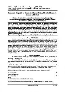
Figure 1. Standard pseudopotential model of a solid. The ion cores composed of the nuclei and tightly bound core electrons are treated as chemically inert. The pseudopotential model describes only the outer, chemically active, valence electrons.

Pseudopotential calculations center on the accuracy of the valence electron wave function in the spatial region away from the core. The smoothly varying pseudo wave function is taken to be identical to the appropriate all-electron wave function in the chemically active bonding regions. A number of schemes have been developed to construct pseudopotentials that yield wave functions of this kind and these will be discussed later. It is interesting to note here that a similar construction was introduced by Fermi in 1934 [3] to account for the shift in the wave functions of high lying states of alkali atoms subject to perturbations from foreign atoms. In this remarkable paper, Fermi introduced the conceptual basis for both the pseudopotential and the scattering length. In Fermi’s analysis, he noted that it was not necessary to know the details of the scattering potential. Any number of potentials which reproduced the phase shifts of interest would yield similar scattering events.


3

2. Constructing Pseudopotentials Most modern pseudopotentials are based on the same idea, but are not fit to experimental data. Rather, they are almost always based on density functional theory[4]. Within this framework, it is easy to apply the pseudopotential approach to a wide variety of problems. A significant advance in the construction of pseudopotentials occurred with the development of density functional theory. Within density functional theory, the many body problem is mapped on to a one-electron Hamiltonian. The effects of exchange and correlation are subsumed into a one electron potential that depends only on the charge density. This procedures allows for a great simplification of the one electron problem. Without this approach most electronic structure methods would not be feasible for systems of more than a few atoms. Again, the roots of this method reside in the early work of Fermi, e.g., the Thomas-Fermi model of the atom[5]. This mapping of the many body problem to a one body problem often incorporates an additional approximation: the local density approximation (LDA)[4]. LDA allows one to construct self-consistent field pseudopotentials for condensed matter systems. The chief limitation of these approximations is that they are appropriate only for the ground state structure and cannot be used to describe excited states without other approximations. As such, one uses LDA to determine structural energies, compressibilities, elastic constants vibrational modes and so on, but not band gaps from the eigenvalue spectra. With respect to band gaps and electronic excitations, it is possible to consider these by implementing linear response theory on top of the standard LDA calculations. I will focus on LDA pseudopotentials in this review, but it should be noted that other density approaches have been implemented. An example is the so-called generalized gradient approximation, GGA[6]. In principle, GGA should always be better than LDA. The additional gradient term in GGA may serve to capture some of the nonlocality one expects within the exchange-correlation potential. At present, it appears clear that GGA significantly improves enthalpy terms and cohesive energies, but does not always improve structural properties when compared to experiment. Implementing GGA is not difficult compared to LDA and, as such, it is gaining in popularity. 2.1. Inverting the Kohn-Sham Equations Let us illustrate the construction procedure for an ab initio pseudopotential within density functional theory. For an isolated atom, one follows the pioneering work of Kohn and Sham[7]. With this approach one can write down a one electron Hamiltonian and the corresponding one-electron Schrödinger equation using the local density approximation. The resulting equation is often called the Kohn-Sham equation: ³ −¯ h2 ∇2

2m

−

´ Ze2 + VH (~r) + Vxc [~r, ρ(~r)] ψn (~r) = En ψn (~r) r

(1)


4

where there are Z electrons in the atom, VH is the Hartree or Coulomb potential, and Vxc is the exchange correlation potential. The Hartree and exchange-correlation potentials can be determined from the electronic charge density. The eigenvalue and eigenfunctions, (En , ψn (~r)), can be used to determine the total electronic energy of the atom. The density is given by ρ(~r) = −e

X

|ψn (~r)|2

(2)

n,occup

The summation is over all occupied states. The Hartree potential is then determined by ∇2 VH (~r) = −4πeρ(~r) (3) This term can be interpreted as the electrostatic interaction of an electron with the charge density of system. The exchange-correlation potential is more problematic. Within density functional theory, one can define an exchange correlation potential as a functional of the charge density. The central tenant of the local density approximation[7] is that the total exchange-correlation energy may be written as Z

Exc [ρ] =

ρ(~r) ²xc (ρ(~r)) d3 r

(4)

where ²xc is the exchange-correlation energy density (i.e. the energy per electron of a homogeneous electron gas). If one has knowledge of the exchange-correlation energy density, one can extract the potential and total electronic energy of the system. It is common practice to separate exchange and correlation contributions to ²xc : ²xc = ²x +²c . It is also convenient to define an electron gas parameter, rs , where rs is given by rs = (

3 )1/3 4πρ(~r)

(5)

A simple form for the exchange part of ²x can be obtained by evaluating the exchange potential for a homogeneous electron gas[8]: ²x (rs ) = −

0.4582 rs

(6)

The correlation contributions to this potential are more problematic. A number of different forms have been proposed for this term. One of the most popular arises from Monte Carlo simulations[9] for free electron gas. The results from the simulation are numerically parameterized for convenient implementation[10]. One commonly used form is −0.1432 ²c (rs ) = for rs ≥ 1 (7) √ 1 + 1.0529 rs + 0.334rs and ²c (rs ) = −0.0480 + 0.0311 ln rs − 0.0116 rs + 0.0020 rs ln rs

for rs < 1

(8)


5

Once the exchange-correlation energy, the potential energy can be obtained from the functional derivative: δExc [rs ] δrs Vxc [~r, ρ(~r)] = · (9) δrs δρ This potential can be explicitly written as Vxc [~r, rs ] = ²xc [~r, rs ] −

rs d²xc ) ( 3 drs

(10)

It is not difficult to solve the Kohn-Sham equation (Eq. 1) for an atom. The charge density is taken to be spherically symmetric. Thus, the problem reduces to solving a one-dimensional problem. The Hartree and exchange-correlation potentials can be iterated to form a self-consistent field. Usually the process is so quick that it can be done on desktop or laptop computer in a matter of seconds. In three dimensions, as for a complex atomic cluster, the problem is highly nontrivial. One major difficulty is the range of length scales involved. For example, in the case of a multi-electron atom, the most tightly bound, core electrons can be confined to within ∼ 0.01 ˚ A whereas the outer valence electron may extend over ∼ 1-5 ˚ A. In addition, the nodal structure of the atomic wave functions are difficult to replicate with a simple basis, especially the wave function cusp at the origin where the Coulomb potential diverges. The pseudopotential approximation eliminates this problem and is quite efficacious when combined with density functional theory. However, it should be noted that the pseudopotential approximation is not dependent on the density functional theory. Pseudopotentials can be created without resort to density functional theory, e.g., pseudopotentials can be created within Hartree-Fock theory. Let us consider a sodium atom for the purposes of designing an ab initio pseudopotential. By solving for the Na atom, we know the eigenvalue, ²3s , and the corresponding wave function, ψ3s (r) for the valence electron. We demand several conditions for the Na pseudopotential: (1) The potential bind only the valence electron, the 3s-electron for the case at hand. (2) The eigenvalue of the corresponding valence electron be identical to the full potential eigenvalue. The full potential is also called the all-electron potential. (3) The wave function be nodeless and identical to the “all electron” wave function outside the core region. For example, we construct a pseudowave function, φ3s (r) such that φ3s (r) = ψ3s (r) for r > rc where rc defines the size spanned by the ion core, i.e., the nucleus and core electrons. For Na, this means the “size” of 1s2 2s2 2p6 states. Typically, the core is taken to be less than the distance corresponding to the maximum of the valence wave function, but greater than the distance of the outermost node. This is depicted in Fig. 2. There are some subtle points involved in this type of construction. For example, insisting that the pseudo-wave function, φp (r), be identical to the all electron wave function, ψAE (r), outside the core: φp (r) = ψAE (r) for r > rc will guarantee that the pseudo-wave function will possess identical properties as the all electron wave function, especially in terms of its chemical bond. For r < rc , we alter the all-electron wave function as we wish within certain limitations. Namely, we want the wave function in


6

0.6

Wave Functions

Na 0.4

3s

3p

0.2

0

-0.2 0

1

2

3

4

5

r (a.u.)

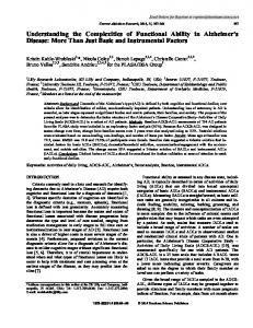
Figure 2. Pseudopotential wave functions compared to all-electron wave functions for the sodium atom. The all-electron wave functions are indicated by the dashed lines.

this region to be smooth and nodeless. Another very important criterion is mandated. Namely, the integral of the pseudocharge density, i.e., square of the wave function |φp (r)|2 , within the core should be equal to the integral of the all-electron charge density. Without this condition, the pseudo-wave function can differ by a scaling factor from the all-electron wave function, that is, φp (r) = C × ψAE (r) for r > rc where the constant, C, may differ from unity. Since we expect the chemical bonding of an atom to be highly dependent on the tails of the valence wave functions, it is imperative that the normalized pseudo wave function be identical to the all-electron wave functions. The criterion by which one insures C = 1 is called norm conserving [11]. Some of the earliest ab initio potentials did not incorporate this constraint. These potentials are not used for accurate computations. The chemical properties resulting from these calculations using these non-norm conserving pseudopotentials are quite poor when compared to experiment or to the more accurate norm conserving pseudopotentials. In 1980, Kerker[12] proposed a straightforward method for constructing local density pseudopotentials that retained the norm conserving criterion. He suggested that the pseudo-wave function have the following form: φp (r) = rl exp (p(r))

for r < rc

(11)

where p(r) is a simple polynomial: p(r) = −a0 r4 − a1 r3 − a2 r2 − a3 and φp (r) = ψAE (r)

for r > rc

(12)

This form of the pseudo-wave function for φp assures us that the function will be nodeless and have the correct behavior at large r. Kerker proposed criteria for fixing


7

the parameters (a0 , a1 , a2 and a3 ). One criterion is that the wave function be norm conserving. Other criteria include: (a) The all electron and pseudo-wave functions have the same valence eigenvalue. (b) The pseudo-wave function be nodeless and be identical to the all-electron wave function for r > rc . (c) The pseudo-wave function must be continuous as well as the first and second derivatives of the wave function at rc . Other local density pseudopotentials include those proposed by Hamann, Schluter, and Chiang[11], Bachelet, Hamann, and Schluter[13] and Greenside and Schluter[14]. These pseudopotentials were constructed from a different perspective. The all-electron potential was calculated for the free atom. This potential was multiplied by a smooth, short range cut-off function which removes the strongly attractive and singular part of the potential. The cut-off function is adjusted numerically to yield eigenvalues equal to the all-electron valence eigenvalues, and to yield nodeless wave functions converged to the all electron wave functions outside the core region. Again, the pseudo-charge within the core is constrained to be equal to the all-electron value. As indicated, there is some flexibility in constructing pseudopotentials. While all local density pseudopotentials impose the condition that φp (r) = ψAE (r) for r > rc , the construction for r < rc . is not unique. The non-uniqueness of the pseudo wave function was recognized early in its inception[2]. This attribute can be exploited to optimize the convergence of the pseudopotentials for the basis of interest. Much effort has been made to construct “soft” pseudopotentials. By soft, one means a rapidly convergent calculation using a simple basis such as plane waves. Typically, soft potentials are characterized by a large core radius, rc . However, as the core becomes larger, the quality of the pseudo-wave function can be compromised. As the core size is increased, the convergence between the all electron and pseudo wave functions is postponed to larger distances. If the core size is too large the quality of the pseudo wave functions starts to deteriorate and the the transferability of the pseudopotential between the atom and condensed matter environments becomes more limited. Several schemes have been developed to generate soft pseudopotentials for species which extend effectively the core radius while preserving transferability. The primary motivation for such schemes is to reduce the size of the basis. One of the earliest discussions of such issues is from Vanderbilt[16]. A common measure of pseudopotential softness is to examine the behavior of the potential in reciprocal space. For example, a hard core pseudopotential, e.g., a non-norm conserving pseudopotential that scales as 1/r2 decays for small r, will decay only as 1/q. This rate of decay is worse than using the bare coulomb potential which scales as 1/q 2 . The Kerker pseudopotential does no better than the coulomb potential as the Kerker pseudopotential has a discontinuity in its third derivative at the origin and at the cut-off radius. This gives rise to a slow 1/q 2 decay of the potential, although one should examine each case, as the error introduced by truncation of such a potential in reciprocal space may still be acceptable in terms of yielding accurate wave functions and energies. Hamann-Schluter-Chiang[11]


8

potentials often converge better than the Kerker potentials[12] in that they contain no such discontinuities. An outstanding issue that remains unresolved is the “best” criterion to use in constructing an “optimal” pseudopotential. An optimal pseudopotential is one that minimizes the number of basis functions required to achieve the desired goal; it yields a converged total energy yet does not sacrifice transferability. One straightforward approach to optimizing a pseudopotential is to build additional constraints into the polynomial given in Eq. (11). For example, suppose we write p(r) = co +

N X

cn r n

(13)

n=1

In Kerker’s scheme, N=4. However, there is no compelling reason for demanding that the series terminate at this particular point. If we extend the expansion, we may impose additional constraints. For example, we might try to constrain the reciprocal space expansion of the pseudo- wave function so that beyond some momentum cut-off the function vanishes. A different approach has been suggested by Troullier and Martins, 1991[15]. They write Eq. 14 as p(r) = co +

6 X

c2n r2n

(14)

n=1

As usual, they constrained the coefficients to be norm conserving. In addition, they demanded continuity of the pseudo-wave functions and the first four derivatives at rc . The final constraint was to demand zero curvature of the pseudopotential at the origin. These potentials tend to be quite smooth and converge very rapidly in reciprocal space. Once the pseudo wave function is defined as in Eqs. (11,12) we can “invert” the Kohn-Sham equation and solve for the ion core pseudopotential, Vion,p : n Vion,p (~r)

h ¯ 2 ∇2 φp,n = En − VH (~r) − Vxc [~r, ρ(~r)] + 2mφp,n

(15)

This potential, when self-consistently screened by the pseudo-charge density: ρ(~r) = − e

X

|φp,n (~r)|2

(16)

n,occup

will yield an eigenvalue of En and a pseudo wave function φp,n . The pseudo wave function by construction will agree with the all electron wave function away from the core. There are some important issues to consider about the details of this construction. First, the potential is state dependent as written in Eq. (15), i.e., the pseudopotential is dependent on the quantum state n. This issue can be handled by recognizing the nonlocality of the pseudopotential. The potential is different for an s-, p-, or d-electron. The nonlocality appears in the angular dependence of the potential, but not in the radial coordinate. A related issue is whether the potential is highly dependent on the state energy, e.g., if the potential is fixed to replicate the 3s state in Na, will it also


9

do well for the 4s, 5s, 6s, etc.? Of course, one could also question how dependent the pseudopotential is on the atomic state used for its construction. For example, would a Na potential be very different for a 3s1 3p0 versus a 3s1/2 3p1/2 configuration? Finally, how important are loosely bound core states in defining the potential? For example, can one treat the 3d states in copper as part of the core or part of the valence shell? Each of this issues has been carefully addressed in the literature. Let us consider the last point first. In most cases, the separation between the core states and the valence states is clear. For example, in Si there is no issue that the core is composed of the 1s2 2s2 p6 states. However, the core in Cu could be considered to be the 1s2 2s2 p6 3s2 3p6 3d10 configuration with the valence shell consisting of the 4s1 state. Alternatively, one could well consider the core to be the 1s2 2s2 p6 3s2 3p6 configuration with the valence shell composed of the 3d10 4s1 states. On physical grounds, it is clear that treating the valence state as a 4s state cannot be correct, otherwise K and Cu would be chemically similar. It is the outer 3d shell that distinguishes Cu from K. Such issues need are traditionally considered on a case by case situation. It is always to construct different pseudopotentials one for each core-valence dichotomy. One can examine the resulting electronic structure for each potential, and verify the role of including a questionable state as a valence or core state. Another aspect of this problem concerns the issue of “core-valence” exchangecorrelation. In the all electron exchange-correlation potential, the charge density is composed of the core and valence states; in the pseudopotential treatment only the valence electrons are included. This separation neglects terms that may arise between the overlap of the valence and core states. There are well defined procedures for including these overlap terms. It is possible to include a fixed charge density from the core and allow the valence overlap to be explicitly included. This procedure is referred to as a partial core correction[17]. This correction is especially important for elements such as Zn, Cd and Hg where the outermost filled d-shell can contribute to the chemical bonding. Again, the importance of this correction can be tested by performing calculations with and without the partial core. Of course, one might argue that the most accurate approach would be to include any “loosely bound” core states as valence states. This approach is often not computationally feasible or desirable. For example, the Zn core without the 3d states results in dealing with an ion core pseudopotential for Zn+12 . This results in a very strong pseudopotential that is required to bind 12 valence electrons. The basis must contain highly localized functions to replicate the d-states plus extended states to replicate the s-states. Moreover, the number of occupied eigenstates increases by a factor of six. Since most “standard” algorithms to solve for eigenvalues scale superlinearly in time with the number of eigenvalues (such as N2eig where Neig is the number of require eigenvalues), this is a serious issue. With respect to the state dependence of the pseudopotential, these problems can be overcome with little computational effort. Since the core electrons are tightly bound, the ion core potential is highly localized and is not highly sensitive to the ground state configuration used to compute the pseudopotential. There are well defined tests for


10

2 1

s-pseudopotential

Potential (Ry)

0 -1 p-pseudopotential

-2 d-pseudopotential

-3 -4

all electron

-5 0

1

2

3

4

r (a.u.)

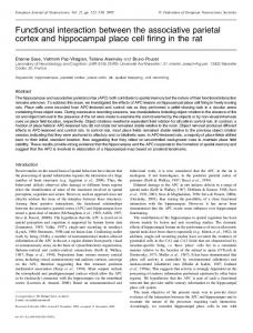
Figure 3. Pseudopotential compared to the all electron potential for the sodium atom.

assessing the accuracy of the pseudopotential, especially in terms of the phase shifts. Also, it should be noted that higher excited states sample the tail of the pseudopotential. This pseudopotential should converge to the all electron potential outside of the core. A significant source of error here is the local density approximation. The LDA yields a potential that scales exponentially at large distances and not as one would expect for an image charge, i.e., the true potential should incorporate an image potential such that Vxc (r → ∞) → −e2 /r. Nonlocality in the pseudopotential is often treated in Fourier space, but it may also be expressed in real space. The interactions between valence electrons and pseudo-ionic cores may be separated into a local potential and a Kleinman and Bylander [18] form of a nonlocal pseudopotential in real space [15], p Vion (~r)φn (~r) =

X

Vloc (|~ra |)φn (~r) +

a

a Kn,lm =

X

Gan,lm ulm (~ra )∆Vl (ra ),

(17)

a, n,lm

Z 1 ulm (~ra )∆Vl (ra )ψn (~r)d3 r, a < ∆Vlm >

(18)

a > is the normalization factor, and < ∆Vlm

=

ulm (~ra )∆Vl (ra )ulm (~ra )d3 r,

(19)

~ a , and the ulm are the atomic pseudopotential wave functions of angular where ~ra = ~r − R momentum quantum numbers (l, m) from which the l-dependent ionic pseudopotential, Vl (r), is generated. ∆Vl (r) = Vl (r) − Vloc (r) is the difference between the l component of the ionic pseudopotential and the local ionic potential. As a specific example, in the case of Na, we might choose the local part of the potential to replicate only the l = 0 component as defined by the 3s state. The nonlocal parts of the potential would


11

then contain only the l = 1 and l = 2 components. In this review, we will focus on electronic materials such as Si and GaAs in this case the angular momentum for higher components than l = 2 are not significant in the ground state. In these systems, one can treat the summation over l = 0, 1, 2 to be complete. The choice of which angular component is chosen for the local part of the potential is somewhat arbitrary. It is often convenient to chose the local potential to correspond to the highest l-component of interest. This avoids any complex projections. Again, these issues can be tested by choosing different components for the local potential. In Fig. 3, the ion core pseudopotential for Na is presented using the TroullierMartins formalism for creating pseudopotentials. The nonlocality of the potential is evident by the existence of the three potentials corresponding to the s-, p- and d-states. 3. Solving the Eigenvalue Problem Once the pseudopotential has been determined, the resulting eigenvalue problem needs to be solved for the system of interest: ³ −¯ h2 ∇2

2m

p (~r) + VH (~r) + Vxc [~r, ρ(~r)] + Vion

´

φn (~r) = En φn (~r)

(20)

p where Vion is the ionic pseudopotential for the system. Since the ion cores can be treated as chemically inert and highly localized, it is a simple matter to write: p Vion (~r) =

X

p ~ a) Vion,a (~r − R

(21)

~a R p where Vion,a is the ion core pseudopotential associated with the atom, a, at a position ~ Ra . At this point, it is worth summarizing the relevant approximations. We have used density functional theory to map the all electron problem into a one electron problem. Commonly the local density approximation is used in this context. We have made the pseudopotential approximation to eliminate the core electrons and allow us to use simple bases to describe the wave functions. Finally, we have used the Born-Oppenheimer approximation to separate the nuclear and electronic degrees of freedom. Of these approximations, the local density approximation is probably the weakest. Once the eigenvalue problem is solved, the total energy of the system, Etot , can be evaluated from

Etot

Z 1Z 3 ~ a ] (22) = En − d rρ(~r)VH (~r)+ d3 rρ(~r)(Exc [~r, ρ(~r)]−Vxc [~r, ρ(~r)])+Ei−i [R 2 occup X

where Ei−i is the ion-ion repulsion. If one knows the behavior of the total energy as a function of atomic positions, it is possible to compute interatomic forces and perform ab initio molecular dynamics. It should be emphasized that LDA is a ground state theory; it is not appropriate to use this approach to describe excited state properties using the


12

eigenvalues. It is appropriate to use this approximation for use with linear response theory to obtain excited state properties as will be outlined later. A major difficulty in solving the eigenvalue problem in Eq. (20) are the length and energy scales involved. The inner (core) electrons are highly localized and tightly bound compared to the outer (valence electrons). A simple basis function approach is frequently ineffectual. For example, a plane wave basis might require 106 waves to represent converged wave functions for a core electron whereas only 102 waves are required for a valence electron[2]. The pseudopotential overcomes this problem by removing the core states from the problem and replacing the all electron potential by one that replicates only the chemically active, valence electron states[2]. By construction, the pseudopotential reproduces the valence state properties such as the eigenvalue spectrum and the charge density outside the ion core. Since the pseudopotential is weak, simple basis sets such as a plane wave basis can be quite effective for crystalline matter. For example, in the case of crystalline silicon only 50-100 plane waves need to be used. The resulting matrix representation of the Schrödinger operator is dense in Fourier (plane wave) space, but it is not formed explicitly. Instead, matrix-vector product operations are performed with the help of fast Fourier transforms (FFT). This approach is akin to spectral techniques used in solving certain types of partial differential equations. The plane wave method uses a basis of the form: X ~ exp(i(~k + G) ~ · ~r) ψ~k (~r) = α(~k, G) (23) ~ G

~ is a reciprocal lattice vector and α(~k, G) ~ represent the where ~k is the wave vector, G coefficients of the basis. In a plane wave basis, the Laplacian term of the Hamiltonian is p represented by a diagonal matrix. The potential term Vtot gives rise to a dense matrix. In real space it is trivial to operate with the potential term which is represented by a diagonal matrix, and in Fourier space it is trivial to operate with the Laplacian term, which is also represented by a diagonal matrix. The use of plane wave bases also leads to natural preconditioning techniques that are obtained by simply employing a matrix obtained from a smaller plane wave basis, neglecting the effect of high frequency terms on the potential. For periodic systems, where ~k is a good quantum number, the plane wave basis coupled to pseudopotentials is quite effective. However, for non-periodic systems such as clusters, liquids or glasses, the plane wave basis must be combined with a supercell method [2]. The supercell repeats the localized configuration to impose periodicity to the system. This preserves the validity of ~k and Bloch’s theorem, which Eq. (23) obeys. There is a parallel to be made with spectral methods that are quite effective for simple periodic geometries, but lose their superiority when more generality is required. In addition to these difficulties the two FFTs performed at each iteration can be costly, requiring n log n operations, where n is the number of plane waves, versus O(N ) for real space methods where N is the number of grid points. Usually, the matrix size N × N is larger than n × n but only within a constant factor. This is exacerbated in high performance environments where FFTs require an excessive amount


13

of communication and are particularly difficult to implement efficiently. Another popular basis employed with pseudopotentials include Gaussian orbitals[19]. Gaussian bases have the advantage of yielding analytical matrix elements provided the potentials are also expanded in Gaussians. However, the implementation of a Gaussian basis is not as straightforward as with plane waves. For example, numerous indices must be employed to label the state, the atomic site, and the Gaussian orbitals employed. On the positive side, a Gaussian basis yields much smaller matrices and requires less memory than plane wave methods. For this reason Gaussians are especially useful for describing transition metal systems. An alternative approach is to avoid the use of a basis. For example, one can use a real space method that avoids the use of plane waves and FFT’s altogether. This approach has become popular and different versions of this general approach have been implemented by several groups. Here we illustrate a particular version of this approach called the Finite-Difference Pseudopotential Method (FDPM)[20]. A real space approach overcomes many of the complications involved with nonperiodic systems, and although the resulting matrices can be larger than with plane waves, they are sparse and the methods are easier to parallelize. Even on sequential machines, we find that real space methods can be an order of magnitude faster than the traditional approach. Our real space algorithms avoid the use of FFT’s by performing all calculations in real physical space instead of Fourier space. A benefit of avoiding FFT’s is that the new approaches have very few global communications. In fact, the only global operation remaining in real space approaches is that of the inner products. These inner products are required when forming the orthogonal basis used in the generalized Davidson procedure as discussed below. Our approach utilizes finite difference discretization on a real space grid. A key aspect to the success of the finite difference method is the availability of higher order finite difference expansions for the kinetic energy operator, i.e., expansions of the Laplacian [21]. Higher order finite difference methods significantly improve convergence of the eigenvalue problem when compared with standard finite difference methods. If one imposes a simple, uniform grid on our system where the points are described in a 2 finite domain by (xi , yj , zk ), we approximate ∂∂xψ2 at (xi , yj , zk ) by M X ∂2ψ = Cn ψ(xi + nh, yj , zk ) + O(h2M +2 ), 2 ∂x n=−M

(24)

where h is the grid spacing and M is a positive integer. This approximation is accurate to O(h2M +2 ) upon the assumption that ψ can be approximated accurately by a power series in h. Algorithms are available to compute the coefficients Cn for arbitrary order in h [21]. With the kinetic energy operator expanded as in Eq. (24), one can set up a oneelectron Schrödinger equation over a grid. One may assume a uniform grid, but this


14

Figure 4. Uniform grid illustrating a typical configuration for examining the electronic structure of a localized system. The gray sphere represents the domain where the wave functions are allowed to be nonzero. The light spheres within the domain are atoms.

is not a necessary requirement. ψ(xi , yj , zk ) is computed on the grid by solving the eigenvalue problem: 

M M X h ¯2  X − Cn1 ψn (xi + n1 h, yj , zk ) + Cn2 ψn (xi , yj + n2 h, zk ) 2m n1 =−M n2 =−M

+

M X



Cn3 ψn (xi , yj , zk + n3 h) + [ Vion (xi , yj , zk )

n3 =−M

+ VH (xi , yj , zk ) + Vxc (xi , yj , zk ) ] ψn (xi , yj , zk ) = En ψn (xi , yj , zk )

(25)

If we have L grid points, the size of the full matrix resulting from the above problem is L × L. The grid we use is based on points uniformly spaced in a three dimensional cube as shown in Fig. 4, with each grid point corresponding to a row in the matrix. However, many points in the cube are far from any atoms in the system and the wave function on these points may be replaced by zero. Special data structures may be used to discard these points and keep only those having a nonzero value for the wave function. The size of the Hamiltonian matrix is usually reduced by a factor of two to three with this strategy, which is quite important considering the large number of eigenvectors which must be saved. Further, since the Laplacian can be represented by a simple stencil, and since all local potentials sum up to a simple diagonal matrix, the Hamiltonian need not be stored. Handling the ionic pseudopotential is complex as it consists of a local and a non-local term (Eqs. (17 )and (18)). In the discrete form, the nonlocal term becomes a sum over all atoms, a, and quantum numbers, (l, m) of rank-one updates: Vion =

X a

Vloc,a +

X a,l,m

T ca,l,m Ua,l,m Ua,l,m

(26)


15

where Ua,l,m are sparse vectors which are only non-zero in a localized region around each atom, ca,l,m are normalization coefficients. There are several difficulties with the eigen problems generated in this application in addition to the size of the matrices. First, the number of required eigenvectors is proportional to the atoms in the system, and can grow up to thousands. Besides storage, maintaining the orthogonality of these vectors can be a formidable task. Second, the relative separation of the eigenvalues becomes increasingly poor as the matrix size increases and this has an adverse effect on the rate of convergence of the eigenvalue solvers. Preconditioning techniques attempt to alleviate this problem. On the positive side, the matrix need not be stored as was mentioned earlier and this reduces storage requirement. In addition, good initial eigenvector estimates are available at each iteration from the previous self-consistency loop. A popular form of extracting the eigenpairs is based on the generalized Davidson [22] method, in which the preconditioner is not restricted to be a diagonal matrix as in the Davidson method. (A detailed description can be found in [23].) Preconditioning techniques in this approach are typically based on filtering ideas and the fact that the Laplacian is an elliptic operator [24]. The eigenvectors corresponding to the few lowest eigenvalues of ∇2 are smooth functions and so are the corresponding wave functions. When an approximate eigenvector is known at the points of the grid, a smoother eigenvector can be obtained by averaging the value at every point with the values of its neighboring points. Assuming a cartesian (x, y, z) coordinate system, the low frequency filter acting on the value of the wave function at the point (i, j, k), which represents one element of the eigenvector, is described by: ψi−1,j,k + ψi,j−1,k + ψi,j,k−1 + ψi+1,j,k + ψi,j+1,k + ψi,j,k+1 ψi,j,k + ) → (ψi,j,k )F iltered 12 2 (27) It is worth mentioning that other preconditioners that have been tried have resulted in mixed success. The use of shift-and-invert [25] involves solving linear systems with A − σI, where A is the original matrix and the shift σ is close to the desired eigenvalue. These methods would be prohibitively expensive in our situation, given the size of the matrix and the number of times that A − σI must be factored. Alternatives based on an approximate factorization such as ILUT [26] are ineffective beyond the first few eigenvalues. Methods based on approximate inverse techniques have been somewhat more successful, performing better than filtering at additional preprocessing and storage cost. Preconditioning ‘interior’ eigenvalues, i.e., eigenvalues located well inside the interval containing the spectrum, is still a very hard problem. Current solutions only attempt to dampen the effect of eigenvalues which are far away from the ones being computed. This is in effect what is achieved by filtering and sparse approximate inverse preconditioning. These techniques do not reduce the number of steps required for convergence in the same way that shift-and-invert techniques do. However, filtering techniques are inexpensive to apply and result in fairly substantial savings in iterations. (


16

4. Properties of Confined Systems: Clusters The electronic and structural properties of atomic clusters stand as one of the outstanding problems in materials physics. Clusters possess properties that are characteristic of neither the atomic nor solid state. For example, the energy levels in atoms may be discrete and well-separated in energy relative to kT . In contrast, solids have continuum of states (energy bands). Clusters may reside between these limits, i.e., the energy levels may be discrete, but with a separation much less than kT . Real space methods are ideally suited for investigating these systems. In contrast to plane wave methods, real space methods can examine non-periodic systems without introducing artifacts such as supercells. Also, one can easily examine charged clusters. In supercell configurations, unless a compensating background charge is added, the Coulomb energy diverges for charged clusters. A closely related issue concerns electronic excitations. In periodic systems, it is nontrivial to consider localized excitation, e.g., with band theory exciting an atom in one cell, excites all atoms in all the equivalent cells. Most common density functional formalisms avoid these issues by considering localized or non-periodic systems[4]. In general, formalisms for extended systems are difficult to pose because of the boundary conditions, e.g. in infinite periodic systems the position operator is not well-defined. 4.1. Structure Perhaps the most fundamental issue in dealing with clusters is determining their structure. Before any accurate theoretical calculations can be performed for a cluster, the atomic geometry of a system must be defined. However, this can be a formidable exercise. Serious problems arise from the existence of multiple local minima in the potential-energy-surface of these systems; many similar structures can exist with vanishingly small energy differences. A complicating issue is the transcription of interatomic forces into tractable classical force fields. This transcription is especially difficult for clusters such as those involving semiconducting species. In these clusters, strong many body forces can exist that preclude the use of pairwise forces. A convenient method to determine the structure of small or moderate sized clusters is simulated annealing[27]. Within this technique, atoms are randomly placed within a large cell and allowed to interact at a high (usually fictive) temperature. The atoms will sample a large number of configurations. As the system is cooled, the number of high energy configurations sampled is restricted. If the anneal is done slowly enough, the procedure should quench out structural candidates for the ground state structures. Langevin molecular dynamics is well suited for simulated annealing methods. In Langevin dynamics, the ionic positions, Rj , evolve according to ¨ j = F({Rj }) − γMj R ˙ j + Gj Mj R

(28)

where F({Rj }) is the interatomic force on the j-th particle, and {Mj } are the ionic masses. The last two terms on the right hand side of Eq. (28) are the dissipation


17

and fluctuation forces, respectively. The dissipative forces are defined by the friction coefficient, γ. The fluctuation forces are defined by random Gaussian variables, {Gi }, with a white noise spectrum: hGαi (t)i = 0 and hGαi (t)Gαj (t0 )i = 2γ Mi kB T δij δ(t − t0 )

(29)

The angular brackets denote ensemble or time averages, and α stands for the Cartesian component. The coefficient of T on the right hand side of Eq. (29) insures that the fluctuation-dissipation theorem is obeyed, i.e., the work done on the system is dissipated by the viscous medium ([28, 29]). The interatomic forces can be obtained from the Hellmann-Feynman theorem using the pseudopotential wave functions. Langevin simulations using quantum forces can be contrasted with other techniques such as the Car-Parrinello method[30]. Langevin simulations as outlined above do not employ fictitious electron dynamics; at each time step the system is quenched to the Born-Oppenheimer surface and the quantum forces are determined. This approach requires a fully-self consistent treatment of the electronic structure problem; however, because the interatomic forces are true quantum forces, the resulting molecular dynamics simulation can be performed with much larger time steps. Typically, it is possible to use steps an order of magnitude larger than in the Car-Parrinello method[31]. It should be emphasized that neither of these methods is particularly efficacious without the pseudopotential approximation. To illustrate the simulated annealing procedure, we consider a silicon cluster of seven atoms. With respect to the technical details for this example, the initial temperature of the simulation was taken to be about 3000 K; the final temperature was taken to be 300 K. The annealing schedule lowered the temperature 500 K each 50 time steps. The time step was taken to be 5 fs. The friction coefficient in the Langevin equation was taken to be 6×10−4 a.u. [1 atomic unit (a.u.) is defined by h ¯ = m = e = 1. The unit of energy is the hartree (1 hartree = 27.2 eV); the unit of length is the bohr radius (1 bohr = 0.529˚ A).] After the clusters reached a temperature of 300 K, they were quenched to 0 K. The ground state structure was found through a direct minimization by a steepest descent procedure. Choosing an initial atomic configuration for the simulation takes some care. If the atoms are too far apart, they will exhibit Brownian motion, which is appropriate for Langevin dynamics with the interatomic forces zeroed. In this case, the atoms may not form a stable cluster as the simulation proceeds. Conversely, if the atoms are too close together, they may form a metastable cluster from which the ground state may be kinetically inaccessible even at the initial high temperature. Often the initial cluster is formed by a random placement of the atoms with a constraint that any given atom must reside within 1.05 and 1.3 times the bond length from at least one atom where the bond the length is defined by the crystalline environment. The cluster in question is placed in a spherical domain. Outside of this domain, the wave function is required to vanish. The radius of the sphere is such that the outmost atom is at least 6 a.u. from the boundary. Initially, the grid spacing was 0.8 a.u. For the final quench to a ground


18

Figure 5. Binding energy of Si7 during a Langevin simulation. The initial temperature is 3000 K; the final temperature is 300 K. Bonds are drawn for interatomic distances of less than 2.5˚ A. The time step is 5 fs.

state structure, the grid spacing was reduced to 0.5 a.u. As a rough estimate, one can compare this grid spacing with a plane wave cutoff of (π/h)2 or about 40 Ry for h=0.5 a.u. In Fig. 5, we illustrate the simulated anneal for the Si7 cluster. The initial cluster contains several incipient bonds, but the structure is far removed from the ground state by approximately 1 eV/atom. In this simulation, at about 100 time steps a tetramer and a trimer form. These units come together and precipitate a large drop in the binding energy. After another ∼100 time steps, the ground state structure is essentially formed. The ground state of Si7 is a bicapped pentagon, as is the corresponding structure for the Ge7 cluster. The binding energy shown in Fig. 5 is relative to that of an isolated Si atom. Gradient corrections[6], or spin polarization[32] haver not been included in this example.. Therefore, the binding energies indicated in the Figure are likely to be overestimated by ∼ 20% or so. In Fig. 6, we present the ground state structures for Sin for n ≤ 7. The structures for Gen are very similar to Sin . The primary difference resides in the bond lengths. The Si bond length in the crystal is 2.35 ˚ A, whereas in Ge the bond length is 2.44 ˚ A. This difference is reflected in the bond lengths for the corresponding clusters; Sin bond lengths are typically a few percent shorter than the corresponding Gen clusters. It should be emphasized that this annealing simulation is an optimization procedure. As such, other optimization procedures may be used to extract the minimum energy structures. Recently, a genetic algorithm has been used to examine carbon clusters [33]. In this algorithm, an initial set of clusters is “mated” with the lowest energy offspring “surviving”. By examining several thousand generations, it is possible


19

Figure 6. Ground state geometries and some low-energy isomers of Sin (n ≤ 7) clusters. Interatomic distances are in ˚ A. The values in parentheses are from Ref. [34].

to extract a reasonable structure for the ground state. The genetic algorithm has some advantages over a simulated anneal, especially for clusters which contain more than ∼20 atoms. One of these advantages is that kinetic barriers are more easily overcome. However, the implementation of the genetic algorithm is more involved than an annealing simulation, e.g., in some cases “mutations,” or ad hoc structural rearrangements, must be introduced to obtain the correct ground state. 4.2. Photoemission Spectra A very useful probe of condensed matter involves the photoemission process. Incident photons are used to eject electrons from a solid. If the energy and spatial distributions of the electrons are known, then information can be obtained about the electronic structure of the materials of interest. For crystalline matter, the photoemission spectra can be


(I)

20

(II)

Figure 7. Two possible isomers for Si10 or Ge10 clusters. (I) is a tri-capped trigonal prism cluster and (II) is a bi-capped anti-prism cluster .

related to the electronic density of states. For confined systems, the interpretation is not as straightforward. One of the earliest experiments performed to examine the electronic structures of small semiconductor clusters examined negatively charged Sin and Gen (n ≤ 12) clusters [35]. The photoemission spectra obtained in this work were used to gauge the energy gap between the highest occupied state and the lowest unoccupied state. Large gaps were assigned to the “magic number” clusters, while other clusters appeared to have vanishing gaps. Unfortunately, the first theoretical estimates [36] for these gaps showed substantial disagreements with the measured values. It was proposed by Cheshnovsky et al. [35], that sophisticated calculations including transition cross sections and final states were necessary to identify the cluster geometry from the photoemission data. The data were first interpreted in terms of the gaps obtained for neutral clusters; it was later demonstrated that atomic relaxations within the charged cluster are important in analyzing the photoemission data [37, 38]. In particular, atomic relaxations as a result of charging may change dramatically the electronic spectra of certain clusters. These charge induced changes in the gap were found to yield very good agreement with the experiment. The photoemission spectrum of Ge− 10 illustrates some of the key issues. Unlike − − Si10 , the experimental spectra for Ge10 does not exhibit a gap. Cheshnovsky et al. − interpreted this to mean that Ge− 10 does not exist in the same structure as Si10 . This is a strange result. Si and Ge are chemically similar and the calculated structures for both neutral structures are similar. The lowest energy structure for both ten atom clusters is the tetracapped trigonal prism (labeled by I in Fig. 7). The photoemission spectra for these clusters can be simulated by using Langevin dynamics. The clusters are immersed in a fictive heat bath, and subjected to stochastic forces. If one maintains the temperature of the heat bath and averages over the eigenvalue spectra, a density


21

of states for the cluster can be obtained. The heat bath resembles a buffer gas as in the experimental setup, but the time intervals for collisions are not similar to the true collision processes in the atomic beam. The simulated photoemission spectrum for Si− 10 is in very good agreement with the experimental results, reproducing both the threshold peak and other features in the spectrum. If a simulation is repeated for Ge− 10 using the tetracapped trigonal prism structure, the resulting photoemission spectrum is not in good agreement with experiment. Moreover, the calculated electron affinity is 2.0 eV in contrast to the experimental value of 2.6 eV. However, there is no reason to believe that the tetracapped trigonal prism structure is correct for Ge10 when charged. In fact, we find that the bicapped antiprism structure is lower in energy for Ge− 10 . The resulting spectra using both structures (I and II in Fig. 7) are presented in Fig. 8, and compared to the photoemission experiment. The calculated spectrum using the bicapped antiprism structure is in very good agreement with the photoemission. The presence of a gap is indicated by a small peak removed from the density of states [Fig. 8(a)]. This feature is absent in the bicapped antiprism structure [Fig. 8(b)] and consistent with experiment. For Ge10 , charging the structure reverses the relative stability of the two structures. This accounts for the major differences between the photoemission spectra. Of course, it is difficult to assign a physical origin to a particular structure owing to the smaller energy differences involved . However, the bicapped structure has a higher coordination. Most chemical theories of bonding suggest that Ge is more metallic than Si, and as such, would prefer a more highly coordinated structure. The addition of an extra electron may induce the more metallic characteristic of Ge. 4.3. Vibrational Modes Experiments on the vibrational spectra of clusters can provide us with very important information about their physical properties. Recently, Raman experiments have been performed on clusters which have been deposited on inert substrates [39]. Since different structural configurations of a given cluster can possess different vibrational spectra, it is possible to compare the vibrational modes calculated for a particular structure with the Raman experiment in a manner similar to the previous example with photoemission. If the agreement between experiment and theory is good, this is a necessary condition for the validity of the theoretically predicted structure. There are two common approaches for determining the vibrational spectra of clusters. One approach is to calculate the dynamical matrix for the ground state structure of the cluster: Miα,jβ

1 ∂2E 1 ∂Fiβ = =− m ∂Riα ∂Rjβ m ∂Rjα

(30)

where m is the mass of the atom, E is the total energy of the system, Fiα is the force on atom i in the direction α, Riα is the α component of coordinate for atom i. One can calculate the dynamical matrix elements by calculating the first order derivative

-6 -5 -4 -3 -2 -1 0 Energy (eV)

(b)

-6 -5 -4 -3 -2 -1 0 Energy (eV)

Photoelectron counts

(a)

DOS (Arbitrary units)

DOS (Arbitrary units)


22

(c)

6 5 4 3 2 1 0 Binding Energy (eV)

Figure 8. Calculated density of states for Ge− 10 in the tetracapped trigonal prism structure (a) and the bicapped antiprism structure (b). (c) Experimental photoemission spectra from Ref. [35].

of force versus atom displacement numerically. From the eigenvalues and eigenmodes of the dynamical matrix, one can obtain the vibrational frequencies and modes for the cluster of interest [40]. The other approach to determine the vibrational modes is to perform a molecular dynamics simulation. The cluster in question is excited by small random displacements. By recording the kinetic (or binding) energy of the cluster as a function of the simulation time, it is possible to extract the power spectrum of the cluster and determine the vibrational modes. This approach has an advantage for large clusters in that one never has to do a mode analysis explicitly. Another advantage is that anaharmonic mode couplings can be examined. It has the disadvantage in that the simulation must be performed over a long time to extract accurate values for all the modes. As a specific example, consider the vibrational modes for a small silicon cluster: Si4 . The starting geometry was taken to be a planar structure for this cluster as established from a higher order finite difference calculation[40]. It is straightforward to determine the dynamical matrix and eigenmodes for this cluster. In Fig. 9, the fundamental vibrational modes are illustrated. In Table 1, the frequency of these modes are presented. One can also determine the modes via a simulation. To initiate the simulation, one can perform a Langevin simulation[37] with a fixed temperature at 300K. After a few dozen time steps, the Langevin simulation is turned off, and the simulation proceeds following Newtonian dynamics with “quantum”


23

Figure 9. Normal modes for a Si4 cluster. The + and − signs indicate motion in and out of the plane, respectively.

forces. This procedure allows a stochastic element to be introduced and establish initial conditions for the simulation without bias toward a particular mode. For this example, time step in the molecular dynamics simulation was taken to be 3.7 fs, or approximately 150 a.u. The simulation was allowed to proceed for 1000 time steps or roughly 4 ps. The variation of the kinetic and binding energies is given in Fig. 10 as a function of the simulation time. Although some fluctuations of the total energy occur, these fluctuations are relatively small, i.e., less than ∼ 1 meV, and there is no noticeable drift of the total energy. Such fluctuations arise, in part, because of discretization errors. As the grid size is reduced, such errors are minimized[40]. Similar errors can occur in plane wave descriptions using supercells, i.e., the artificial periodicity of the supercell can introduce erroneous forces on the cluster. By taking the power spectrum of either the kinetic energy (KE) or binding energy (BE) over this simulation time, the vibrational modes can be determined. These modes can be identified with the observed peaks in the power spectrum as illustrated in Fig. 11. A comparison of the calculated vibrational modes from the molecular dynamics simulation and from a dynamical matrix calculation are listed in Table 1. Overall, the agreement between the simulation and the dynamical matrix analysis is quite satisfactory. In particular, the softest mode, i.e., the B3u mode, and the splitting between the (Ag , B1u ) modes are well replicated in the power spectrum. The splitting of the (Ag , B1u ) modes is less than 10 cm−1 , or about 1 meV, which is probably at the resolution limit of any ab initio method. The theoretical values are also compared to experiment. The predicted frequencies for the two Ag modes are surprisingly close to Raman experiments on silicon clusters[39]. The other allowed Raman line of mode B3g is expected to have a lower intensity and


24

Figure 10. Simulation for a Si4 cluster. The kinetic energy (KE) and binding energy (BE) are shown as a function of simulation time. The total energy (KE+BE) is also shown with the zero of energy taken as the average of the total energy. The time step, ∆t, is 3.7fs.

Figure 11. Power spectrum of the vibrational modes of the Si4 cluster. The simulation time was taken to be 4 ps. The intensity of the B3g and (Ag ,B1u ) peaks has been scaled by 10−2 .


25

Table 1. Calculated and experimental vibrational frequencies in a Si4 cluster. See Figure 9 for an illustration of the normal modes. The frequencies are given in cm−1 .

Experiment[39] Dynamical Matrix [40] MD simulation [40] HF[42] LCAO[41]

B3u

B2u

160 150 117 55

280 250 305 248

Ag 345 340 340 357 348

B3g 460 440 465 436

Ag B1u 470 480 500 490 500 489 529 464 495

has not been observed experimentally. The theoretical modes using the formalism outlined here are in good accord (except the lowest mode) with other theoretical calculations given in Table 1: an LCAO calculation [41] and a Hartree-Fock (HF) calculation[42]. The calculated frequency of the lowest mode, i.e., the B3u mode, is problematic. The general agreement of the B3u mode as calculated by the simulation and from the dynamical matrix is reassuring. Moreover, the real space calculations agree with the HF value to within ∼ 20-30 cm−1 . On the other hand, the LCAO method yields a value which is 50 − 70% smaller than either the real space or HF calculations. The origin of this difference is not apparent. For a poorly converged basis, vibrational frequencies are often overestimated as opposed to the LCAO result which underestimates the value, at least when compared to other theoretical techniques. Setting aside the issue of the B3u mode, the agreement between the measured Raman modes and theory for Si4 suggests that Raman spectroscopy can provide a key test for the structures predicted by theory. 4.4. Polarizabilities Recently polarizability measurements [43] have been performed for small semiconductor clusters. These measurements will allow one to compare computed values with experiment. The polarizability tensor, αij , is defined as the second derivative of the energy with respect to electric field components. For a noninteracting quantum mechanical system, the expression for the polarizability can be easily obtained by using second order perturbation theory where the external electric field, E, is treated as a weak perturbation. Within the density functional theory, since the total energy is not the sum of individual eigenvalues, the calculation of polarizability becomes a nontrivial task. One approach is to use density functional perturbation theory which has been developed recently in Green’s function and variational formulations[44, 45]. Another approach, which is very convenient for handling the problem for confined systems, like clusters, is to solve the full problem exactly within the one electron


26

Figure 12. One component of the polarizability tensor of Si7 as a function of the electric field. The dashed curve is the polarizability component from the second derivative of the energy with respect to the field; the solid curve is from the dipole derivative. For very small fields, the values are not accurate owing to the strict convergence criteria required in the wave functions to get accurate values. For high fields, the cluster is ionized. The dashed value is the predicted value for the cluster using a small, but finite field.

approximation. In this approach, the external ionic potential Vion (r) experienced by the electrons is modified to have an additional term given by −eE · r. The Kohn-Sham equations are solved with the full external potential Vion (r) − eE · r. For quantities like polarizability, which are derivatives of the total energy, one can compute the energy at a few field values, and differentiate numerically. Real space methods are very suitable for such calculations on confined systems, since the position operator r is not ill-defined, as is the case for supercell geometries in plane wave calculations. There is another point that should be emphasized. It is difficult to determine the polarizability of a cluster or molecule owing to the need for a complete basis in the presence of an electric field. Often polarization functions are added to complete a basis and the response of the system to the field can be sensitive to the basis required. In both real space and plane wave methods, the lack of a “prejudice” with respect to the


27

Table 2. Static dipole moments and average polarizabilities of small silicon and germanium clusters.

cluster Si2 Si3 Si4 Si5 Si6 (I) Si6 (II) Si7

Silicon |µ| hαi 3 (D) (˚ A /atom) 0 6.29 0.33 5.22 0 5.07 0 4.81 0 4.46 0.19 4.48 0 4.37

Germanium cluster |µ| hαi 3 (D) (˚ A /atom) Ge2 0 6.67 Ge3 0.43 5.89 Ge4 0 5.45 Ge5 0 5.15 Ge6 (I) 0 4.87 Ge6 (II) 0.14 4.88 Ge7 0 4.70

basis are considerable assets. The real space method implemented with a uniform grid possesses a nearly “isotropic” environment with respect to the applied field. Moreover, the response can be easily checked with respect to the grid size by varying the grid spacing. Typically, the calculated electronic response of a cluster is not sensitive to the magnitude of the field over several orders of magnitude. In Fig. 12, we illustrate the calculated polarizability as a function of the finite electric fields. For very small fields, the polarizability calculated by the change in dipole or energy is not reliable because of numerical inaccuracies such as roundoff errors. For very large fields, the cluster can be ionized by the field and again the accuracy suffers. However, for a wide range of values of the electric field, the calculated values are stable. In Table 2, we present some recent calculations for the polarizability of small Si and Ge clusters. (This procedure has recently been extended to heteropolar clusters such as Gam Asn , see [46]) It is interesting to note that some of these clusters have permanent dipoles. For example, Si6 and Ge6 both have nearly degenerate isomers. One of these isomers possesses a permanent dipole, the other does not. Hence, in principle, one might be able to separate the one isomer from the other via an inhomogeneous electric field. 4.5. Optical Spectra While the theoretical background for calculating ground state properties of manyelectron systems is now well established, excited state properties such as optical spectra present a challenge for density functional theory. Recently developed linear response theory within the time-dependent density-functional formalism provides a new tool for calculating excited states properties [47]. This method, known as the timedependent LDA (TDLDA), allows one to compute the true excitation energies from the conventional, time independent Kohn-Sham transition energies and wave functions. Within the TDLDA, the electronic transition energies Ωn are obtained from the


28

solution of the following eigenvalue problem:[47] · 2 ωijσ δik δjl δστ

¸

q

q

+ 2 fijσ ωijσ Kijσ,klτ fklτ ωklτ Fn = Ω2n Fn

(31)

where ωijσ = ²jσ − ²iσ are the Kohn-Sham transition energies, fijσ = niσ − njσ are the differences between the occupation numbers of the i-th and j-th states, the eigenvectors Fn are related to the transition oscillator strengths, and Kijσ,klτ is a coupling matrix given by: ZZ

Kijσ,klτ =

Ã

φ∗iσ (r)φjσ (r)

!

1 ∂vσxc (r) φkτ (r0 )φ∗lτ (r0 )drdr0 + 0 0 |r − r | ∂ρτ (r )

(32)

where i, j, σ are the occupied state, unoccupied state, and spin indices respectively, φ(r) are the Kohn-Sham wave functions, and v xc (r) is the LDA exchange-correlation potential. The TDLDA formalism is easy to implement in real space within the higherorder finite difference pseudopotential method [20]. The real-space pseudopotential code represents a natural choice for implementing TDLDA due to the real-space formulation of the general theory. With other methods, such as the plane wave approach, TDLDA calculations typically require an intermediate real-space basis. After the original plane wave calculation has been completed, all functions are transferred into that basis, and the TDLDA response is computed in real space [48]. The additional basis complicates calculations and introduces an extra error. The real-space approach simplifies implementation and allows us to perform the complete TDLDA response calculation in a single step. I illustrate the TDLDA technique by calculating the absorption spectra of a sodium cluster. Sodium clusters were chosen as well-studied objects, for which accurate experimental measurements of the absorption spectra are available [49]. The groundstate structures of the clusters were determined by simulated annealing [37]. In all cases the obtained cluster geometries agreed well with the structures reported in other works [50]. Since the wave functions for the unoccupied electron states are very sensitive to the boundary conditions, TDLDA calculations need to be performed within a relatively large boundary domain. For sodium clusters we used a spherical domain with a radius of 25 a.u. and a grid spacing of 0.9 a.u. We carefully tested convergence of the calculated excitation energies with respect to these parameters. The calculated absorption spectrum for Na4 is shown in Fig. 13 along with experiment. In addition, we illustrate the spectrum generated by considering transitions between the LDA eigenvalues. The agreement between TDLDA and experiment is remarkable, especially when contrasted with the LDA spectrum. TDLDA correctly reproduces the experimental spectral shape, and the calculated peak positions agree with experiment within 0.1 − 0.2 eV. The comparison with other theoretical work demonstrates that our TDLDA absorption spectrum is as accurate as the available CI spectra [51]. Furthermore, the TDLDA spectrum for the Na4 cluster seems to be in


Na4

a) Absorption cross section (arbitrary units)

29

b)

c)

0

1

2

3

4

Energy (eV) Figure 13. The calculated and experimental absorption spectrum for Na4 . (a) shows a local density approximation to the spectrum using Kohn-Sham eigenvalues. (b) shows a TDLDA calculation. Technical details of the calculation can be found in [53]. (c) panel is experiment from[49].

better agreement with experiment than the GW absorption spectrum calculated in Ref. [52]. 5. Quantum Confinement Thus far, I have focused on the electronic properties of small clusters. There are two reasons for this. First, these clusters are quite tractable with pseudopotential methods, e.g., simulated annealing methods can be used to predict their structures. Second,


30

experimental data are available for a wide variety of properties. However, large clusters are also interesting, especially clusters whose surfaces are passivated and retain the structure of the crystalline host. These clusters are called quantum dots. Understanding the role of quantum confinement (QC) in altering optical properties of quantum dots made from semiconductor materials is a problem of both technological and fundamental interest. In particular, the discovery of visible luminescence from porous Si [54] has focused attention on optical properties of confined systems. Although there is still debate on the exact mechanism of photoluminescence in porous Si, there is a great deal of experimental and theoretical evidence that supports the important role played by QC in producing this phenomenon [55, 56]. Excitations in confined systems, like Si quantum dots as the building blocks of porous Si, differ from those in extended systems due to QC. In particular, the components that comprise the excitation energies, such as quasiparticle and exciton binding energies change significantly with the physical extent of the system. So far, most calculations that model semiconductor quantum dots have been of an empirical nature owing to major challenges to simulate these systems from first principles[57-61]. While empirical studies have shed some light on the physics of optical excitations in semiconductor quantum dots, one often has to make assumptions and approximations that may or may not be justified. Efficient and accurate ab initio studies are necessary to achieve a better microscopic understanding of the size dependence of optical processes in semiconductor quantum dots. A major goal of our work is to develop such ab initio methods that handle systems from atoms to dots to crystals on an equal footing. A problem using empirical approaches for semiconductor quantum dots centers on the transferability of the bulk interaction parameters to the nanocrystalline environment. The validity of this assumption, which postulates the use of fitted bulk parameters in a size regime of a few nanometers, is not clear, and has been questioned in recent studies [62]. More specifically, QC-induced changes in the self-energy corrections, which may affect the magnitude of the optical gaps significantly, are neglected in empirical approaches by implicitly assuming a “size-independent” correction that corresponds to that of the bulk. It follows that a reliable way to investigate optical properties of quantum dots would be to model them from first principles with no uncontrolled approximations or empirical data. However, there have been two major obstacles for the application of ab initio studies to these systems. First, due to large computational demand, accurate first principles calculations have been limited to small system sizes, which do not correspond to the nanoparticle sizes for which experimental data are available. Second, even accurate ab initio calculations performed within the local density approximation (LDA) suffer from the underestimate of the band gap [63]. Recent advances in electronic structure algorithms using pseudopotentials (as outlined earlier) [20, 64] and computational platforms, and alternative formulations of the optical gaps suitable for confined systems, the above-mentioned challenges for ab initio studies of quantum dots can be overcome. In particular, the use of the higherorder finite difference pseudopotential method [20], implemented on massively parallel


31

Figure 14. Atomic structure of a Si quantum dot with composition Si525 H276 . The gray and white balls represent Si and H atoms, respectively. This bulk-truncated Si quantum dot contains 25 shells of Si atoms and is 27.2 ˚ A in diameter.

computational platforms allows us to model a cluster of more than 1,000 atoms in a straightforward fashion [65]. As for the second problem regarding the underestimate of the band gap due to LDA, the confined nature of the quantum dots makes it possible for an alternative formulation of the fundamental quasiparticle gaps. We can outline this approach by focusing on silicon quantum dots such as Si705 H300 . This system corresponds to spherically bulk-terminated Si clusters passivated by hydrogens at the boundaries, Fig. 14. Troullier-Martins pseudopotentials [15] in nonlocal [18] and local forms for Si and H, respectively yield very accurate and rapidly convergent results. All calculations for these systems were performed within LDA using the exchange correlation functional of Ceperley and Alder [9]. The kinetic energy in the finite difference expression is typically expanded up to twelfth order with a grid spacing h of 0.9 a.u. We found no changes in the calculated gap values upon decreasing h to 0.75 a.u. The wave functions were required to vanish outside a spherical domain, which was at least 7.5 a.u. away from the last shell of Si atoms. For systems of this size, one uses a generalized Davidson algorithm with dynamical residual tolerance to diagonalize the matrix of interest. Typically, 10 to 15 diagonalizations are needed to obtain the self-consistent charge density irrespective of the size of the system. The Hartree potential for such dots is solved by discretizing the Poisson equation and matching the boundary potential with that of a multipole


32

Table 3. HOMO-LUMO and quasiparticle gaps εqp (Eq. 1) calculated for g hydrogenated Si clusters compared to quasiparticle gaps calculated within the GW approximation [67]. All energies are in eV.

SiH4 Si2 H6 Si5 H12 Si14 H20

εHL g 7.9 6.7 6.0 4.4

εqp g 12.3 10.7 9.5 7.6

GW 12.7 10.6 9.8 8.0

expansion of the charge density with angular momentum l = 9 to 20. We have considered quantum dots containing 65 to 1,005 atoms requiring the self-consistent solutions of 100 to 1,700 eigenpairs. With the grid spacing and domain size chosen as described above, the Hamiltonian sizes range from 25,000 to 250,000. For an n−electron system, the quasiparticle gap εqp g can be expressed in terms of the ground state total energies E of the (n + 1)−, (n − 1)−, and n−electron systems as HL εqp g = E(n + 1) + E(n − 1) − 2E(n) = εg + Σ

(33)

where Σ is the self-energy correction to the HOMO-LUMO gap εHL obtained within g LDA. This definition is quite convenient for the calculation of the quasiparticle gap, as it is possible to excite individual electrons or holes from the ground state electronic configuration of a confined system. The calculation of εqp g requires the selfconsistent solutions of three different charge configurations of each quantum dot. The computational demand of this approach can be reduced significantly by using the wave functions of the neutral cluster to extract very good initial charge densities for the selfconsistent solutions of the charged systems. With a real-space method, total energies for charged (n + 1)− and (n − 1)−electron systems can be calculated in a straightforward fashion without the need for a compensating background charge that would be necessary for plane wave calculations with a supercell geometry. Eq. (33) yields the correct quasiparticle gap εqp g , if the exact exchange-correlation functional is used. Within LDA, in the limit of very large systems (n → ∞), the gaps calculated using Eq. (33) approach the HOMO-LUMO gap εHL [66]. However, g for small systems, Eq. (33) captures the correction to the LDA HOMO-LUMO gap quite accurately (Table 3 ) when compared with available GW calculations [67]. Small deviations appear as the system size reaches approximately 1,000 atoms in our calculations. The size dependence of the quasiparticle and LDA HOMO-LUMO gaps, and selfenergy corrections are shown in Fig. 15. Both gap values and self-energy corrections are enhanced substantially with respect to bulk values, and are inversely proportional to the


33

7 Quasiparticle HOMO-LUMO Self-Energy

Energy (eV)

6 5 4 3 2 1 10

14 18 22 26 30 Quantum dot diameter (A)

Figure 15. Calculated quasiparticle (¦) and HOMO-LUMO gaps (+), and self-energy corrections (×) as a function of the quantum dot diameter d (in ˚ A). The solid lines are power-law fits to the calculated data approaching the corresponding bulk limits. For small deviations from the fits for large system sizes, see the text.

qp band quantum dot diameter d as a result of QC. Specifically, εqp (d) − εband g (d) − εg,bulk , εg g,bulk , −1.2 −1.1 −1.5 and Σ(d) − Σbulk scale as d , d , and d , respectively. The quasiparticle gaps shown in the figure are significantly higher compared to the gap values obtained in earlier semi-empirical calculations, although it is problematic in terms of any comparisons. The empirical gaps are obtained from potentials obtained from crystalline environments and scaled to dot sizes. The nature of these gaps is problematic in that they do not strictly correspond to quasiparticle gaps owing to their empirical roots. The main reason for the size difference in the gaps is the significant enhancement of electron self-energies due to QC, which cannot be properly taken into account in semi-empirical approaches. Since the quasiparticle gap refers to the energy to create a non-interacting electronhole (e − h) pair, one cannot compare these gaps directly to measurements of the optical gap. This issue is especially important for quantum dots in which the exciton radius becomes comparable to the size of the dot. QC in nanostructures enhances the bare exciton Coulomb interaction, and also reduces the electronic screening so that the exciton Coulomb energy ECoul becomes comparable to the quasiparticle gap. In order to extract the optical gaps: εopt = εqp (34) g g − ECoul

the exciton Coulomb energy needs to be calculated accurately. Compared to ECoul , exciton exchange-correlation energies are much smaller for the quantum dots studied in this work, and will therefore be neglected. Eq.(34) is a rigorous expression, provided the Coulomb energy can be properly computed. A crude, yet commonly used, approximation to ECoul comes from the effective mass approximation (EMA) [68]. In the EMA, one assumes (i) an infinite potential barrier at the boundary of the quantum dot, and (ii) envelope wave functions of


34

the form ψ(r) ∼ 1r sin(2πr)/d for a noninteracting e − h pair. This yields (in a.u.) ECoul = 3.572/²d. EMA, though commonly used, cannot be expected to yield accurate exciton Coulomb energies, since in this approximation the microscopic features of the electron-hole wave functions inside the quantum dot are neglected, and the wave functions are constrained to vanish abruptly outside the quantum dots, instead of decaying relatively slowly into the vacuum. Thus, ECoul is better calculated directly using ab initio pseudo wave functions. The exciton Coulomb energy can be written as Z

h ECoul = dr1 |ψe (r1 )|2 Vscr (r1 )

Z

Z

h (r) = dr1 |ψe (r1 )|2 dr²−1 (r1 , r)Vunscr

ZZZ

=

²−1 (r1 , r)

|ψe (r1 )|2 |ψh (r2 )|2 dr dr1 dr2 . |r − r2 |

(35)

h h In this expression, Vscr and Vunscr are screened and unscreened potentials due to the hole, ψe and ψh are the electron and hole wave functions, and ²−1 is the inverse of the microscopic dielectric matrix. We may formally define ²˜−1 as Z 1 1 dr ≡ ²˜−1 (r1 , r2 ) , (36) ²−1 (r1 , r) |r − r2 | |r1 − r2 |

then the exciton Coulomb energy can be written as ZZ

ECoul =

²˜−1 (r1 , r2 )

|ψe (r1 )|2 |ψh (r2 )|2 dr1 dr2 . |r1 − r2 |

(37)

If we set ²˜ = 1, the unscreened ECoul can be determined. The results are shown in Fig. 16 along with the predictions of the EMA and recent empirical calculations [69]. The ab initio and empirical calculations for the unscreened Coulomb energy are in quite good agreement with each other, both predicting smaller Coulomb energies and a softer power-law decay compared to the EMA. In particular, fitting the calculated data to a power law of the diameter as d−β , we find β = 0.7. An accurate calculation of ECoul requires the inverse dielectric matrix ²˜−1 (r1 , r2 ) in Eq. (37). An ab initio calculation of ²˜−1 (r1 , r2 ) is computationally very demanding. Earlier calculations used either the bulk dielectric constant or the reduced dielectric constant of the quantum dot for all e − h distances. These are rather simple approximations, since the screening is different at different length scales owing to the wave vector dependence of ²˜. For example, when r1 and r2 in Eq. (37) are very close to each other, there will be practically no screening, and ²˜ ≈ 1. Typically, both the hole and electron wave functions are well localized towards the center of the quantum dot, the screening will be reduced significantly, resulting in larger Coulomb energies compared to the case of using a single dielectric constant for all distances. Also, extracting the appropriate dielectric constant for these small systems is problematic. One can improve on these approximations by explicitly using the wave functions as calculated by our pseudopotential approach and a realistic dielectric function that takes spatial variations of ²˜ into account. To calculate the screening dielectric functions

Unscreened Coulomb Energy (eV


35

6 Ab initio Empirical EMA

5 4 3 2 1 10


Figure 16. Unscreened exciton Coulomb energies as a function of the quantum dot diameter d (in ˚ A) calculated by (i) effective mass approximation (dashed line), (ii) direct empirical pseudopotential calculations (4 from Ref. [69]), (iii) direct ab initio pseudopotential calculations (×) as explained in the text. The solid lines are power-law fits to the calculated data.

²˜(r1 , r2 ) of a particular quantum dot, one can proceed as follows: First, one applies a spatially modulated electric fields at several wave vectors to calculate the q−dependent polarizability α(q) using a finite-field method. The q−dependent dielectric function ²˜(q) can be obtained using a dielectric sphere model [46]. The results for ²˜(q) of the Si87 H76 quantum dot are shown in Fig. 17. After fitting the calculated ²˜(q) to a rational polynomial function of q and Fourier-transforming to real space [70], we obtained the dielectric function ²˜(r = |r1 −r2 |). Implicitly, we are assuming spatial isotropy in writing ²˜(r1 , r2 ) ≈ ²˜(r = |r1 − r2 |). As shown in Fig. 17, the calculated ²˜(q) has a very sharp drop to ≈ 1 beyond q = 0.2 a.u., which corresponds roughly to the wavevector set by the linear dimension (or diameter) of this quantum dot. This sharp drop is typical for all quantum dots studied. In real space, this implies that the e − h interaction is very inefficiently screened inside the dot resulting in substantial excitonic Coulomb energies. The resulting optical gaps εopt = εqp g g − ECoul along with the quasiparticle gaps and experimental absorption data [71] from Si:H nanocrystals are shown in Fig. 18. Although the calculated quasiparticle gaps are ∼ 0.6 to 1.0 eV larger than the experimental absorption data, the calculated optical gaps are in very good agreement with experiment. At this point, an interesting observation can be made about the good agreement of previous semi-empirical calculations with experiment [55, 57, 59]. In the above semiempirical approaches, it is the underestimate of both the excitation gap and the exciton Coulomb energies (through the use of a static dielectric constant of either the bulk or the quantum dot), that results in calculated values in agreement with experiment. As a matter of fact, the bare gaps of Refs. [57] and [59] without the exciton Coulomb


36

5

Epsilon(q)

4 3 2 1 0.0

0.2

0.4 0.6 q (a.u.)

0.8

1.0

Figure 17. Wavevector dependence of the dielectric function for the Si87 H76 quantum dot.

6 Quasiparticle Experiment Experiment Optical

Energy (eV)

5 4 3 2 10


Figure 18. Calculated quasiparticle gaps (dotted line), optical gaps, and experimental absorption data from Si:H nanocrystals (× and ¦ from Ref. [71]) as a function of the quantum dot diameter d (in ˚ A). The two sets of experimental data (× and ¦) differ by the method to estimate the nanocrystal size.

energies are in better agreement with the experiment. The ab initio pseudopotential results demonstrate that (i) the quasiparticle gaps in Si quantum dots are actually higher than previously thought, and (ii) the exciton Coulomb energies, because of the wavevector dependence of the dielectric response function ²(r1 , r2 ), are higher than previously calculated, resulting in optical gap values that are in good agreement with the experimental absorption data.


37

6. Acknowledgments I would like to acknowledge support from the National Science Foundation, the United States Department of Energy and the Minnesota Supercomputing Institute. 7. References [1] J.R. Chelikowsky and S.G. Louie, editors, Quantum Theory of Real Materials, (Kluwer Press, Boston), 1996. [2] J.R. Chelikowsky, and M.L. Cohen: “Ab initio Pseudopotentials for Semiconductors,” Handbook on Semiconductors, Editor: Peter Landsberg, (Elsevier, 1992), Vol. 1, p. 59. [3] E. Fermi, Nuovo Cimento 11, 157 (1934). [4] P. Hohenberg and W. Kohn, Phys. Rev. 136, B864 (1964); W. Kohn and L. Sham, Phys. Rev. A 140, 1133 (1965); S. Lundqvist and N.H. March, editors, Theory of the Inhomogeneous Electron Gas, (Plenum, New York), 1983; R.G. Parr and W. Yang, Density Functional Theory of Atoms and Molecules, (Oxford, New York), 1989. [5] L.H. Thomas, Proc. Camb. Phil. Soc 23, 542 (1926); E. Fermi, Z. Phys. 48, 73 (1928). [6] J.P. Perdew, K. Burke, and Y. Wang, Phys. Rev. B54, 16533 (1996); A.B. Becke, J. Chem. 98, 5648 (1993) and references therein. [7] W. Kohn and L. Sham, Phys. Rev. A 140, 1133 (1965). [8] N.W. Aschroft and N.D. Mermin, Solid State Physics, (Holt Rinehart an Winston, New York), 1976, contains a nice derivation for ²x . [9] D.M. Ceperley and B.J. Alder, Phys. Rev. Lett. 45, 566 (1980) [10] J. P. Perdew and A. Zunger, Phys. Rev. B 23, 5048 (1981). [11] D.R. Hamann, M. Schl¨ uter, and C. Chiang, Phys. Rev. Lett. 43, 1494 (1979). [12] G.P. Kerker, J. Phys. C 13, L189 (1980). [13] G. Bachelet, D.R. Hamann and M. Schl¨ uter, Phys. Rev. B 26, 4199 (1982). [14] H.S. Greenside and M. Schl¨ uter, Phys. Rev. B 28, 535 (1983). [15] N. Troullier, and J.L. Martins, Phys. Rev. B43, 1993 (1991). [16] D. Vanderbilt, Phys. Rev. B 41, 7892 (1990). [17] S.G. Louie, S. Froyen, and M.L. Cohen, Phys. Rev. B 26, 1738 (1982). [18] L. Kleinman and D.M. Bylander, Phys. Rev. Lett. 48, 1425 (1982). [19] See for examples: A. Briley, M.R. Pederson, K.A. Jackson, D.C. Patton, and D.V. Porezag, Phys. Rev. B 58, 1786 (1997); K.A. Jackson, M.R. Pederson, D.V. Porezag, Z. Hajnal and Th. Fraunheim, Phys. Rev. B 55, 2549 (1997); J. R. Chelikowsky and S.G. Louie, Phys. Rev. B 29, 3470 (1984); R.W. Jansen and O.F. Sankey, Phys. Rev. B 36, 6520 (1987) and references therein. [20] J.R. Chelikowsky, N. Troullier, and Y. Saad, Phys. Rev. Lett., 72, 1240 (1994); J.R. Chelikowsky, N. Troullier, K. Wu, and Y. Saad, Phys. Rev. B 50, 11355 (1994); J.R. Chelikowsky, N. Troullier, X. Jing, D. Dean, N. Binggeli, K. Wu and Y. Saad, Computer Physics Communications 85,325 (1995); J.R. Chelikowsky, N. Troullier, K. Wu, and Y. Saad: “Algorithms for Predicting Properties of Real Materials on High Performance Computers,” Proceedings of the “Toward Teraflop Computing Conference and New Grand Challenge Applications,” Baton Rouge, LA 1994, editors: R.K. Kalia and P. Vashista, (Nova, New York), 1995, p. 13; J.R. Chelikowsky, X. Jing, K. Wu and Y. Saad, Phys. Rev. B 53, 12071 (1996). [21] B. Fornberg and D. M. Sloan, Acta Numerica 94, Editor A. Iserles, Cambridge University Press, 1994. [22] R.B. Morgan and D.S. Scott, SIAM J. Sci. Stat. Comput. 7, 817 (1986). ¨ gu [23] Y. Saad, A. Stathopoulos, J.R. Chelikowsky, K. Wu and S. O˘ ¨t, BIT 36, 563 (1996). [24] C.H. Tong, T.F. Chan and C.C. J. Kuo, SIAM J. Sci. Stat. Comput. 13, 227 (1992).

The Pseudopotential-Density Functional Method Applied to Nanostructures [25] [26] [27] [28] [29] [30] [31] [32] [33] [34]

[35] [36] [37] [38] [39] [40]

[41] [42] [43] [44] [45] [46] [47]

[48] [49] [50] [51] [52] [53] [54] [55] [56] [57] [58] [59] [60] [61] [62]

38

B.N. Parlett, The Symmetric Eigenvalue Problem, (Prentice Hall, Englewood Cliffs), 1980. Y. Saad, Iterative Methods for Sparse Linear Systems, (PWS Publishing Company, Boston), 1196. R. Biswas and D.R. Hamann, Phys. Rev. B 34, 895 (1986). R. Kubo, Rep. Prog. Theor. Phys. 29, 255, (1966). H. Risken, The Fokker-Planck Equation (Springer-Verlag, Berlin),1984. R. Car and Parrinello, Phys. Rev. Lett. 55, 2471 (1985); 60 204 (1988). N. Binggeli, J.L. Martins, and J.R. Chelikowsky: “Simulation of Si Clusters via Langevin Molecular Dynamics with Quantum Forces,” Phys. Rev. Lett. 68, 2956 (1992). F.W. Kutzler and G.S. Painter, Phys. Rev. B 45, 3236 (1992). D. Deaven and K.M. Ho, Phys. Rev. Lett. 75, 288 (1995). C. Rohlfing and K. Raghavachari, J. Chem. Phys. 96, 2114 (1992); K. Raghavachari and V. Logovinsky, Phys. Rev. Lett. 55, 2853 (1985); K. Raghavachari and C. Rohlfing, J. Chem. Phys. 94, 3670 (1990). O. Cheshnovsky, S.H. Yang, C.L. Pettiett, M.J. Craycraft, Y. Liu, and R.E. Smalley, Chem. Phys. Lett. 138, 119 (1987). D. Tomanek and M. Schl¨ uter, Phys. Rev. Lett. 56, 1055 (1986). N. Binggeli and J.R. Chelikowsky, Phys. Rev. B 50, 11764(1994). ¨ gu S. O˘ ¨t and J.R. Chelikowsky, Phys. Rev. B 55, R4914 (1997) E.C. Honea, A. Ogura, C.A. Murray, K.Raghavachari, O. Sprenger, M.F. Jarrold, and W.L. Brown, Nature 366, 42 (1993). X. Jing, N. Troullier, J.R. Chelikowsky, K. Wu and Y. Saad, Solid State Comm. 96, 231 (1995) and X. Jing, N. Troullier, D. Dean, N. Binggeli, J.R. Chelikowsky, K. Wu, and Y. Saad: “ Ab Initio Molecular Dynamics Simulations of Si Clusters Using a High-Order Finite-DifferencePseudopotential Method,” Phys. Rev. B 50, 12234 (1994). R. Fournier, S.B. Sinnott, and A.E. DePristo, J. Chem. Phys. 97, 4149 (1992). C. Rohlfing and K. Raghavachari, J. Chem. Phys. 96, 2114 (1992). R. Sch¨ afer, S. Schlect, J., Woenckhaus and J.A. Becker, Phys. Rev. Lett. 76, 471(1996). S. Baroni, P. Gianozzi and A. Testa, Phys. Rev. Lett. 58, 1861 (1987). X. Gonze, D.C. Allan and M.P. Teter, Phys. Rev. Lett. 68, 3603 (1992). ¨ gu I. Vasiliev, S. O˘ ¨t and J.R. Chelikowsky, Phys. Rev. Lett. 78, 4805 (1997). M. E. Casida, in Recent Advances in Density-Functional Methods, edited by D. P. Chong (World Scientific, Singapore, 1995), Part I, Chap. 5; in Recent Developments and Applications of Modern Density Functional Theory, edited by J. M. Seminario (Elsevier, Amsterdam, 1996). X. Blase, A. Rubio, S. G. Louie, and M. L. Cohen, Phys. Rev. B 52, R2225 (1995). C.RC. Wang, S. Pollack, D. Cameron and M.M. Kappes, Chem. Phys. Lett. 93, 3787 (1990) I. Moullet, J. L. Martins, F. Reuse, and J. Buttet, Phys. Rev. B 42, 11598 (1990); J. L. Martins, J. Buttet, and R. Car, Phys. Rev. B 31, 1804 (1985). V. Bonacic-Koutecky, P. Fantucci, and J. Koutecky, J. Chem. Phys. 93, 3802 (1990); Chem. Phys. Lett. 166, 32 (1990). G. Onida, L. Reining, R.W. Godby, R. del Sole and W. Andreoni, Phys. Rev. Lett. 75, 181 (1995). ¨ gu Igor Vasiliev, S. O˘ ¨t, J.R. Chelikowsky, Phys. Rev. Lett. 82, 1919 (1999). L. T. Canham, Appl. Phys. Lett. 57, 1046 (1990). D. J. Lockwood, Solid State Commun. 92, 101 (1994). M. V. Wolkin, J. Jorne, P. M. Fauchet, G. Allan, C. Delerue, Phys. Rev. Lett. 82, 197 (1999). J. P. Proot, C. Delerue, and G. Allan, Appl. Phys. Lett. 61, 1948 (1992); C. Delerue, G. Allan, and M. Lannoo, Phys. Rev. B 48, 11 024 (1993). T. Takagahara and K. Takeda, Phys. Rev. B 46, 15 578 (1992). L. W. Wang and A. Zunger, J. Phys. Chem. 98, 2158 (1994). N. A. Hill and K. B. Whaley, Phys. Rev. Lett. 75, 1130 (1995); ibid. 76, 3039 (1996). C. Delerue, M. Lannoo, and G. Allan, Phys. Rev. Lett. 76, 3038 (1996). M. Lannoo, C. Delerue, and G. Allan, Phys. Rev. Lett. 74, 3415 (1995); G. Allan, C. Delerue, M.


39

Lannoo, and E. Martin, Phys. Rev. B 52, 11 982 (1995). [63] M. S. Hybertsen and S. G. Louie, Phys. Rev. B 34, 5390 (1986). [64] E. L. Briggs, D. J. Sullivan, and J. Bernholc, Phys. Rev. B 52, R5471 (1995); F. Gygi and G. Galli, ibid., R2229 (1995); G. Zumbach, N. A. Modine, E. Kaxiras, Solid State Commun. 99, 57 (1996). ¨ gu [65] S. O˘ ¨t, J. R. Chelikowsky, and S. G. Louie, Phys. Rev. Lett. 79, 1770 (1997). ¨ gu [66] R. W. Godby and I. White, Phys. Rev. Lett. 80, 3161 (1998); S. O˘ ¨t, J. R. Chelikowsky, and S. G. Louie, ibid., 3162 (1998). [67] M. Rohlfing and S. G. Louie, Phys. Rev. Lett. 80, 3320 (1998); private communication. [68] L. Brus, J. Phys. Chem. 90, 2555 (1986); Y. Kayanuma, Phys. Rev. B 38, 9797 (1988). [69] A. Franceschetti and A. Zunger, Phys. Rev. Lett. 78, 915 (1997). [70] G. Srinivasan, Phys. Rev. 178, 1244 (1969). [71] S. Furukawa and T. Miyasato, Phys. Rev. B 38, 5726 (1988).

The Pseudopotential-Density Functional Method ... - Semantic Scholar

The Pseudopotential-Density Functional Method ... - Semantic Scholar

Suggest Documents

A new method for purification of functional ... - Semantic Scholar

An Incremental Slicing Method for Functional ... - Semantic Scholar

The Slack Method - Semantic Scholar

The Teaspoon Method - Semantic Scholar

Functional Programming - Semantic Scholar

Functional Starters for Functional Yogurt - Semantic Scholar

Process Method - Semantic Scholar

Proposed method - Semantic Scholar

The Dynamical Functional Particle Method

Iteration Method - Semantic Scholar

Comparison of the Functional microRNA ... - Semantic Scholar

Functional programming through the curriculum - Semantic Scholar

FUNCTIONAL-COGNITIVE FRAMEWORK Why the ... - Semantic Scholar

VASCULAR DIVERSITY AND THE FUNCTIONAL ... - Semantic Scholar

Functional Genomic Approaches Using the ... - Semantic Scholar

Understanding the Complexities of Functional ... - Semantic Scholar

The TGFB1 Functional Polymorphism rs1800469 ... - Semantic Scholar

Functional Characterization of the Drosophila ... - Semantic Scholar

The Functional Analysis of Histone ... - Semantic Scholar

The Functional Neuroanatomy of Temporal ... - Semantic Scholar

The Functional Significance of Common ... - Semantic Scholar

Functional polymorphisms of the glutamate ... - Semantic Scholar

Functional interaction between the associative ... - Semantic Scholar

Functional Conservation of the Drosophila ... - Semantic Scholar