Perception & Psychophysics 2001, 63 (8), 1314-1329
The psychometric function: II. Bootstrap-based confidence intervals and sampling FELIX A. WICHMANN and N. JEREMY HILL University of Oxford, Oxford, England The psychometric function relates an observer’s performance to an independent variable, usually a physical quantity of an experimental stimulus. Even if a model is successfully fit to the data and its goodness of fit is acceptable, experimenters require an estimate of the variability of the parameters to assess whether differences across conditions are significant. Accurate estimates of variability are difficult to obtain, however, given the typically small size of psychophysical data sets: Traditional statistical techniques are only asymptotically correct and can be shown to be unreliable in some common situations. Here and in our companion paper (Wichmann & Hill, 2001), we suggest alternative statistical techniques based on Monte Carlo resampling methods. The present paper’s principal topic is the estimation of the variability of fitted parameters and derived quantities, such as thresholds and slopes. First, we outline the basic bootstrap procedure and argue in favor of the parametric, as opposed to the nonparametric, bootstrap. Second, we describe how the bootstrap bridging assumption, on which the validity of the procedure depends, can be tested. Third, we show how one’s choice of sampling scheme (the placement of sample points on the stimulus axis) strongly affects the reliability of bootstrap confidence intervals, and we make recommendations on how to sample the psychometric function efficiently. Fourth, we show that, under certain circumstances, the (arbitrary) choice of the distribution function can exert an unwanted influence on the size of the bootstrap confidence intervals obtained, and we make recommendations on how to avoid this influence. Finally, we introduce improved confidence intervals (bias corrected and accelerated) that improve on the parametric and percentile-based bootstrap confidence intervals previously used. Software implementing our methods is available.
The performance of an observer on a psychophysical task is typically summarized by reporting one or more response thresholds—stimulus intensities required to produce a given level of performance—and by a characterization of the rate at which performance improves with increasing stimulus intensity. These measures are derived from a psychometric function, which describes the dependence of an observer’s performance on some physical aspect of the stimulus. Fitting psychometric functions is a variant of the more general problem of modeling data. Modeling data is a Part of this work was presented at the Computers in Psychology (CiP) Conference in York, England, during April 1998 (Hill & Wichmann, 1998). This research was supported by a Wellcome Trust Mathematical Biology Studentship, a Jubilee Scholarship from St. Hugh’s College, Oxford, and a Fellowship by Examination from Magdalen College, Oxford, to F.A.W. and by a grant from the Christopher Welch Trust Fund and a Maplethorpe Scholarship from St. Hugh’s College, Oxford, to N.J.H. We are indebted to Andrew Derrington, Karl Gegenfurtner, Bruce Henning, Larry Maloney, Eero Simoncelli, and Stefaan Tibeau for helpful comments and suggestions. This paper benefited considerably from conscientious peer review, and we thank our reviewers, David Foster, Stan Klein, Marjorie Leek, and Bernhard Treutwein, for helping us to improve our manuscript. Software implementing the methods described in this paper is available (MATLAB); contact F.A.W. at the address provided or see http://users.ox.ac.uk/~sruoxfor/psychofit /. Correspondence concerning this article should be addressed to F. A. Wichmann, Max-PlanckInstitut für Biologische Kybernetik, Spemannstraße 38, D-72076 Tübingen, Germany (e-mail:
[email protected]).
Copyright 2001 Psychonomic Society, Inc.
three-step process: First, a model is chosen, and the parameters are adjusted to minimize the appropriate error metric or loss function. Second, error estimates of the parameters are derived and third, the goodness of fit between model and the data is assessed. This paper is concerned with the second of these steps, the estimation of variability in fitted parameters and in quantities derived from them. Our companion paper (Wichmann & Hill, 2001) illustrates how to fit psychometric functions while avoiding bias resulting from stimulus-independent lapses, and how to evaluate goodness of fit between model and data. We advocate the use of Efron’s bootstrap method, a particular kind of Monte Carlo technique, for the problem of estimating the variability of parameters, thresholds, and slopes of psychometric functions (Efron, 1979, 1982; Efron & Gong, 1983; Efron & Tibshirani, 1991, 1993). Bootstrap techniques are not without their own assumptions and potential pitfalls. In the course of this paper, we shall discuss these and examine their effect on the estimates of variability we obtain. We describe and examine the use of parametric bootstrap techniques in finding confidence intervals for thresholds and slopes. We then explore the sensitivity of the estimated confidence interval widths to (1) sampling schemes, (2) mismatch of the objective function, and (3) accuracy of the originally fitted parameters. The last of these is particularly important, since it provides a test of the validity of the bridging as-
1314
THE PSYCHOMETRIC FUNCTION II sumption on which the use of parametric bootstrap techniques relies. Finally, we recommend, on the basis of the theoretical work of others, the use of a technique called bias correction with acceleration (BCa ) to obtain stable and accurate confidence interval estimates. BACKGROUND The Psychometric Function Our notation will follow the conventions we have outlined in Wichmann and Hill (2001). A brief summary of terms follows. Performance on K blocks of a constant-stimuli psychophysical experiment can be expressed using three vectors, each of length K. An x denotes the stimulus values used, an n denotes the numbers of trials performed at each point, and a y denotes the proportion of correct responses (in n-alternative forced-choice [n-AFC] experiments) or positive responses (single-interval or yes/no experiments) on each block. We often use N to refer to the total number of trials in the set, N 5 åni. The number of correct responses yi ni in a given block i is assumed to be the sum of random samples from a Bernoulli process with probability of success pi. A psychometric function y (x) is the function that relates the stimulus dimension x to the expected performance value p. A common general form for the psychometric function is
(
)
(
) (
)
y x; a , b , g , l = g + 1 - g - l F x; a , b .
(1)
The shape of the curve is determined by our choice of a functional form for F and by the four parameters {a, b, g, l}, to which we shall refer collectively by using the parameter vector q. F is typically a sigmoidal function, such as the Weibull, cumulative Gaussian, logistic, or Gumbel. We assume that F describes the underlying psychological mechanism of interest: The parameters g and l determine the lower and upper bounds of the curve, which are affected by other factors. In yes/no paradigms, g is the guess rate and l the miss rate. In n-AFC paradigms, g usually reflects chance performance and is fixed at the reciprocal of the number of intervals per trial, and l reflects the stimulus-independent error rate or lapse rate (see Wichmann & Hill, 2001, for more details). When a parameter set has been estimated, we will usually be interested in measurements of the threshold (displacement along the x-axis) and slope of the psychometric function. We calculate thresholds by taking the inverse of F at a specified probability level, usually .5. Slopes are calculated by finding the derivative of F with respect to x, evaluated at a specified threshold. Thus, we shall use the 21 , and notation threshold 0.8, for example, to mean F 0.8 21 . When we use the slope0.8 to mean dF/dx evaluated at F0.8 terms threshold and slope without a subscript, we mean threshold 0.5 and slope0.5: In our 2AFC examples, this will mean the stimulus value and slope of F at the point where performance is approximately 75% correct, although the
1315
exact performance level is affected slightly by the (small) value of l. Where an estimate of a parameter set is required, given a particular data set, we use a maximum-likelihood search algorithm, with Bayesian constraints on the parameters based on our beliefs about their possible values. For example, l is constrained within the range [0, .06], reflecting our belief that normal, trained observers do not make stimulus-independent errors at high rates. We describe our method in detail in Wichmann and Hill (2001). Estimates of Variability: Asymptotic Versus Monte Carlo Methods In order to be able to compare response thresholds or slopes across experimental conditions, experimenters require a measure of their variability, which will depend on the number of experimental trials taken and their placement along the stimulus axis. Thus, a fitting procedure must provide not only parameter estimates, but also error estimates for those parameters. Reporting error estimates on fitted parameters is unfortunately not very common in psychophysical studies. Sometimes probit analysis has been used to provide variability estimates (Finney, 1952, 1971). In probit analysis, an iteratively reweighted linear regression is performed on the data once they have undergone transformation through the inverse of a cumulative Gaussian function. Probit analysis relies, however, on asymptotic theory: Maximum-likelihood estimators are asymptotically Gaussian, allowing the standard deviation to be computed from the empirical distribution (Cox & Hinkley, 1974). Asymptotic methods assume that the number of datapoints is large; unfortunately, however, the number of points in a typical psychophysical data set is small (between 4 and 10, with between 20 and 100 trials at each), and in these cases, substantial errors have accordingly been found in the probit estimates of variability (Foster & Bischof, 1987, 1991; McKee, Klein, & Teller, 1985). For this reason, asymptotic theory methods are not recommended for estimating variability in most realistic psychophysical settings. An alternative method, the bootstrap (Efron, 1979, 1982; Efron & Gong, 1983; Efron & Tibshirani, 1991, 1993), has been made possible by the recent sharp increase in the processing speed of desktop computers. The bootstrap method is a Monte Carlo resampling technique relying on a large number of simulated repetitions of the original experiment. It is potentially well suited to the analysis of psychophysical data, because its accuracy does not rely on large numbers of trials, as do methods derived from asymptotic theory (Hinkley, 1988). We apply the bootstrap to the problem of estimating the variability of parameters, thresholds, and slopes of psychometric functions, following Maloney (1990), Foster and Bischof (1987, 1991, 1997), and Treutwein (1995; Treutwein & Strasburger, 1999). The essence of Monte Carlo techniques is that a large number, B, of “synthetic” data sets y1*, …, yB* are generated. For each data set yi*, the quantity of interest J (thresh-
1316
WICHMANN AND HILL
old or slope, e.g.) is estimated to give Jˆ i*. The process for obtaining Jˆi* is the same as that used to obtain the first estiqˆ ), mate Jˆ. Thus, if our first estimate was obtained by Jˆ 5 t(q ˆ q where is the maximum-likelihood parameter estimate from a fit to the original data y, so the simulated estiqˆ i*), where qˆ i* is the mates Jˆ i* will be given by Jˆ i* 5 t(q maximum-likelihood parameter estimate from a fit to the simulated data yi*. Sometimes it is erroneously assumed that the intention is to measure the variability of the underlying J itself. This cannot be the case, however, because repeated computer simulation of the same experiment is no substitute for the real repeated measurements this would require. What Monte Carlo simulations can do is estimate the variability inherent in (1) our sampling, as characterized by the distribution of sample points (x) and the size of the samples (n), and (2) any interaction between our sampling strategy and the process used to estimate J —that is, assuming a model of the observer’s variability, fitting a qˆ ). function to obtain qˆ , and applying t(q Bootstrap Data Sets: Nonparametric and Parametric Generation In applying Monte Carlo techniques to psychophysical data, we require, in order to obtain a simulated data set yi*, some system that provides generating probabilities p for the binomial variates yi1*, …, yiK*. These should be the same generating probabilities that we hypothesize to underlie the empirical data set y. Efron’s bootstrap offers such a system. In the nonparametric bootstrap method, we would assume p 5 y. This is equivalent to resampling, with replacement, the original set of correct and incorrect responses on each block of observations j in y to produce a simulated sample yij*. Alternatively, a parametric bootstrap can be performed. In the parametric bootstrap, assumptions are made about the generating model from which the observed data are believed to arise. In the context of estimating the variability of parameters of psychometric functions, the data are generated by a simulated observer whose underlying probabilities of success are determined by the maximumqˆ )]. likelihood fit to the real observer’s data [yfit 5 y (x;q Thus, where the nonparametric bootstrap uses y, the parametric bootstrap uses yf it as generating probabilities p for the simulated data sets. As is frequently the case in statistics, the choice of parametric versus nonparametric analysis concerns how much confidence one has in one’s hypothesis about the underlying mechanism that gave rise to the raw data, as against the confidence one has in the raw data’s precise numerical values. Choosing the parametric bootstrap for the estimation of variability in psychometric function fitting appears the natural choice for several reasons. First and foremost, in fitting a parametric model to the data, one has already committed oneself to a parametric analysis. No additional assumptions are required to perform a parametric bootstrap beyond those required for fitting a function to the data: Specification of the source of vari-
ability (binomial variability) and the model from which the data are most likely to come (parameter vector q and distribution function F ). Second, given the assumption that data from psychophysical experiments are binomially distributed, we expect data to be variable (noisy). The nonparametric bootstrap treats every datapoint as if its exact value reflected the underlying mechanism.1 The parametric bootstrap, on the other hand, allows the datapoints to be treated as noisy samples from a smooth and monotonic function, determined by q and F. One consequence of the two different bootstrap regimes is as follows. Assume two observers performing the same psychophysical task at the same stimulus intensities x and assume that it happens that the maximum-likelihood fits to the two data sets yield identical parameter vectors q. Given such a scenario, the parametric bootstrap returns identical estimates of variability for both observers, since it depends only on x, q, and F. The nonparametric bootstrap’s estimates would, on the other hand, depend on the individual differences between the two data sets y1 and y2, something we consider unconvincing: A method for estimating variability in parameters and thresholds should return identical estimates for identical observers performing the identical experiment.2 Treutwein (1995) and Treutwein and Strasburger (1999) used the nonparametric bootstrap and Maloney (1990) used the parametric bootstrap to compare bootstrap estimates of variability with real-word variability in the data of repeated psychophysical experiments. All of the above studies found bootstrap studies to be in agreement with the human data. Keeping in mind that the number of repeats in the above-quoted cases was small, this is nonetheless encouraging, suggesting that bootstrap methods are a valid method of variability estimation for parameters fitted to psychophysical data. Testing the Bridging Assumption qˆ will conAsymptotically—that is, for large K and N—q verge toward q, since maximum-likelihood estimation is asymptotically unbiased3 (Cox & Hinkley, 1974; Kendall & Stuart, 1979). For the small K typical of psychophysical experiments, however, we can only hope that our estimated parameter vector qˆ is “close enough” to the true parameter vector q for the estimated variability in the parameter vector qˆ obtained by the bootstrap method to be valid. We call this the bootstrap bridging assumption. Whether qˆ is indeed sufficiently close to q depends, in a complex way, on the sampling—that is, the number of blocks of trials (K ), the numbers of observations at each block of trials (n), and the stimulus intensities (x) relative to the true parameter vector q. Maloney (1990) summarized these dependencies for a given experimental design by plotting the standard deviation of bˆ as a function of a and b as a contour plot (Maloney, 1990, Figure 3, p. 129). Similar contour plots for the standard deviation of aˆ and for bias in both aˆ and bˆ could be obtained. If, owing to small K, bad sampling, or otherwise, our estimation procedure is inaccurate, the distribution of bootstrap param-
THE PSYCHOMETRIC FUNCTION II eter vectors qˆ 1*, …, qˆ B*—centered around qˆ —will not be centered around true q. As a result, the estimates of variability are likely to be incorrect unless the magnitude of the standard deviation is similar around qˆ and q, despite the fact that the points are some distance apart in parameter space. One way to assess the likely accuracy of bootstrap estimates of variability is to follow Maloney (1990) and to examine the local flatness of the contours around qˆ , our best estimate of q. If the contours are sufficiently flat, the variability estimates will be similar, assuming that the true q is somewhere within this flat region. However, the process of local contour estimation is computationally expensive, since it requires a very large number of complete bootstrap runs for each data set. A much quicker alternative is the following. Having obqˆ ) as the tained qˆ and performed a bootstrap using y (x;q generating function, we move to eight different points f1, …, f8 in a–b space. Eight Monte Carlo simulations are performed, using f1, …, f8 as the generating functions to explore the variability in those parts of the parameter space (only the generating parameters of the bootstrap are changed x remains the same for all of them). If the contours of variability around qˆ are sufficiently flat, as we hope they are, confidence intervals at f1, …, f8 should be of the same magnitude as those obtained at qˆ . Prudence should lead us to accept the largest of the nine confidence intervals obtained as our estimate of variability. A decision has to be made as to which eight points in a–b space to use for the new set of simulations. Generally, provided that the psychometric function is at least reasonably well sampled, the contours vary smoothly in the immediate vicinity of q, so that the precise placement of the sample points f1, …, f8 is not critical. One suggested and easy way to obtain a set of additional generating parameters is shown in Figure 1. Figure 1 shows B 5 2,000 bootstrap parameter pairs as dark filled circles plotted in a–b space. Simulated data sets were generated from ygen with the Weibull as F and qgen 5 {10, 3, 0.5, 0.01}; sampling scheme s7 (triangles; see Figure 2) was used, and N was set to 480 (ni 5 80). The large central triangle at (10, 3) marks the generating parameter set; the solid and dashed line segments adjacent to the x- and y-axes mark the 68% and 95% confidence intervals for a and b, respectively.4 In the following, we shall use WCI to stand for width of confidence interval, with a subscript denoting its coverage percentage—that is, WCI68 denotes the width of the 68% confidence interval.5 The eight additional generating parameter pairs f1, …, f8 are marked by the light triangles. They form a rectangle whose sides have length WCI68 in a and b. Typically, this central rectangular region contains approximately 30%– 40% of all a–b pairs and could thus be viewed as a crude joint 35% confidence region for a and b. A coverage percentage of 35% represents a sensible compromise between erroneously accepting the estimate around qˆ , very likely underestimating the true variability, and performing ad-
1317
ditional bootstrap replications too far in the periphery, where variability and, thus, the estimated confidence intervals become erroneously inflated owing to poor sampling. Recently, one of us (Hill, 2001b) performed Monte Carlo simulations to test the coverage of various bootstrap confidence interval methods and found that the above method, based on 25% of points or more, was a good way of guaranteeing that both sides of a two-tailed confidence interval had at least the desired level of coverage. MONTE CARLO SIMULATIONS In both our papers, we use only the specific case of the 2AFC paradigm in our examples: Thus, g is fixed at .5. In our simulations, where we must assume a distribution of true generating probabilities, we always use the Weibull function in conjunction with the same fixed set of generating parameters qgen: {agen 5 10, bgen 5 3, ggen 5 .5, l gen 5 .01}. In our investigation of the effects of sampling patterns, we shall always use K 5 6 and ni constant—that is, six blocks of trials with the same number of points in each block. The number of observations per point, ni, could be set to 20, 40, 80, or 160, and with K 5 6, this means that the total number of observations N could take the values 120, 240, 480, and 960. We have introduced these limitations purely for the purposes of illustration, to keep our explanatory variables down to a manageable number. We have found, in many other simulations, that in most cases this is done without loss of generality of our conclusions. Confidence intervals of parameters, thresholds, and slopes that we report in the following were always obtained using a method called bias-corrected and accelerated (BCa ) confidence intervals, which we describe later in our Bootstrap Confidence Intervals section. The Effects of Sampling Schemes and Number of Trials One of our aims in this study was to examine the effect of N and one’s choice of sample points x on both the size of one’s confidence intervals for Jˆ and their sensitivity to errors in qˆ . Seven different sampling schemes were used, each dictating a different distribution of datapoints along the stimulus axis; they are the same schemes as those used and described in Wichmann and Hill (2001), and they are shown in Figure 2. Each horizontal chain of symbols represents one of the schemes, marking the stimulus values at which the six sample points are placed. The different symbol shapes will be used to identify the sampling schemes in our results plots. To provide a frame of reference, the solid curve shows the psychometric function used—that is, 0.5 1 0.5F(x;{agen, bgen})—with the 55%, 75%, and 95% performance levels marked by dotted lines. As we shall see, even for a fixed number of sample points and a fixed number of trials per point, biases in parameter estimation and goodness-of-fit assessment
1318
WICHMANN AND HILL 8
95% confidence interval 68% confidence interval (WCI68) 7
N = 480 u = {10, 3, 0.5, 0.01}
parameter b
6
5
4
3
2
1
8
9
10
parameter a
11
12
Figure 1. B 5 2,000 data sets were generated from a two-alternative forced-choice Weibull psychometric function with parameter vector qgen 5 {10, 3, .5, .01} and then fit using our maximum-likelihood procedure, resulting in 2,000 estimated parameter pairs (aˆ , bˆ ) shown as dark circles in a–b parameter space. The location of the generating a and b (10, 3) is marked by the large triangle in the center of the plot. The sampling scheme s7 was used to generate the data sets (see Figure 2 for details) with N 5 480. Solid lines mark the 68% confidence interval width (WCI68) separately for a and b; broken lines mark the 95% confidence intervals. The light small triangles show the a–b parameter sets f1, …, f8 from which each bootstrap is repeated during sensitivity analysis while keeping the x-values of the sampling scheme unchanged.
(companion paper), as well as the width of confidence intervals (this paper), all depend markedly on the distribution of stimulus values x. Monte Carlo data sets were generated using our seven sampling schemes shown in Figure 2, using the generation parameters qgen, as well as N and K as specified above. A maximum-likelihood fit was performed on each simulated data set to obtain bootstrap parameter vectors qˆ *, from which we subsequently derived the x values corresponding to threshold 0.5 and threshold 0.8, as well as to the slope. For each sampling scheme and value of N, a total of nine simulations were performed: one at qgen and eight more at points f1, …, f8 as specified in our section on the bootstrap bridging assumption. Thus, each of our 28 conditions (7 sampling schemes 3 4 values of N ) required 9 3 1,000 simulated data sets, for a total of 252,000 simulations, or 1.134 3 108 simulated 2AFC trials.
Figures 3, 4, and 5 show the results of the simulations dealing with slope0.5, threshold 0.5, and threshold 0.8, respectively. The top-left panel (A) of each figure plots the WCI68 of the estimate under consideration as a function of N. Data for all seven sampling schemes are shown, using their respective symbols. The top-right hand panel (B) plots, as a function of N, the maximal elevation of the WCI68 encountered in the vicinity of qgen—that is, max{WCIf1/WCIqgen, …, WCIf8/WCIqgen}. The elevation factor is an indication of the sensitivity of our variability estimates to errors in the estimation of q. The closer it comes to 1.0, the better. The bottom-left panel (C) plots the largest of the WCI68’s measurements at qgen and f1, …, f8 for a given sampling scheme and N; it is, thus, the product of the elevation factor plotted in panel B by its respective WCI68 in panel A. This quantity we denote as MWCI68, standing for maximum width of the
THE PSYCHOMETRIC FUNCTION II
1319
1
proportion correct
.9 .8 .7 .6 .5
s7 s6 s5 s4 s3 s2 s1
.4 .3 .2 .1 0
4
5
7
10
12
15 17
20
signal intensity Figure 2. A two-alternative forced-choice Weibull psychometric function with parameter vector q 5 {10, 3, .5, 0} on semilogarithmic coordinates. The rows of symbols below the curve mark the x values of the seven different sampling schemes, s1–s7, used throughout the remainder of the paper.
68% confidence interval; this is the confidence interval we suggest experimenters should use when they report error bounds. The bottom-right panel (D), finally, shows MWCI68 multiplied by a sweat factor, Ïw Nw /1w 2w 0. Ideally— that is, for very large K and N—confidence intervals should be inversely proportional to Ïw N, and multiplication by our sweat factor should remove this dependency. Any change in the sweat-adjusted MWCI68 as a function of N might thus be taken as an indicator of the degree to which sampling scheme, N, and true confidence interval width interact in a way not predicted by asymptotic theory. Figure 3A shows the WCI68 around the median estimated slope. Clearly, the different sampling schemes have a profound effect on the magnitude of the confidence intervals for slope estimates. For example, in order to ensure that the WCI68 is approximately 0.06, one requires nearly 960 trials if using sampling s1 or s4. Sampling schemes s3, s5, or s7, on the other hand, require only around 200 trials to achieve similar confidence interval width. The important difference that makes, for example, s3, s5, and s7 more efficient than s1 and s4 is the presence of samples at high predicted performance values (p $ .9) where binomial variability is low and, thus, the data constrain our maximum-likelihood fit more tightly. Figure 3B illustrates the complex interactions between different sampling schemes, N, and the stability of the bootstrap estimates of variability, as indicated by the local flatness of the contours around qgen. A perfectly flat local contour would result in the horizontal line at 1. Sampling scheme s6 is well behaved for N $ 480, its maximal elevation being around 1.7. For N , 240, however, elevation rises to near
2.5. Other schemes, like s1, s4, or s7, never rise above an elevation of 2 regardless of N. It is important to note that the magnitude of WCI68 at qgen is by no means a good predictor of the stability of the estimate, as indicated by the sensitivity factor. Figure 3C shows the MWCI68, and here the differences in efficiency between sampling schemes are even more apparent than in Figure 3A. Sampling schemes s3, s5, and s7 are clearly superior to all other sampling schemes, particularly for N , 480; these three sampling schemes are the ones that include two sampling points at p . .92. Figure 4, showing the equivalent data for the estimates of threshold0.5, also illustrates that some sampling schemes make much more efficient use of the experimenter’s time by providing MWCI68s that are more compact than others by a factor of 3.2. Two aspects of the data shown in Figure 4B and 4C are important. First, the sampling schemes fall into two distinct classes: Five of the seven sampling schemes are almost ideally well behaved, with elevations barely exceeding 1.5 even for small N (and MWCI68 # 3); the remaining two, on the other hand, behave poorly, with elevations in excess of 3 for N , 240 (MWCI68 . 5). The two unstable sampling schemes, s1 and s4, are those that do not include at least a single sample point at p $ .95 (see Figure 2). It thus appears crucial to include at least one sample point at p $ .95 to make one’s estimates of variability robust to small errors in qˆ , even if the threshold of interest, as in our example, has a p of only approximately .75. Second, both s1 and s4 are prone to lead to a serious underestimation of the true width of the confidence interval
1320
WICHMANN AND HILL
sampling schemes s2
s3
s4
A
slope WCI68
0.15
0.1
0.05
s5
maximal elevation of WCI68
s1
s6
s7
B 2.5
2
1.5
120 240 480 960 total number of observations N
120 240 480 960 total number of observations N
C
D
0.15
0.1
0.05
120 240 480 960 total number of observations N
sqrt(N/120)*slope MWCI68
slope MWCI68
1
0.25 0.2 0.15 0.1
120 240 480 960 total number of observations N
Figure 3. (A) The width of the 68% BCa confidence interval (WCI68) of slopes of B 5 999 fitted psychometric functions to parametric bootstrap data sets generated from qgen 5 {10, 3, .5, .01} as a function of the total number of observations, N. (B) The maximal elevation of the WCI68 in the vicinity of qgen, again as a function of N (see the text for details). (C) The maximal width of the 68% BCa confidence interval (MWCI68) in the vicinity of qgen,—that is, the product of the respective WCI68 and elevations factors of panels A and B. (D) MWCI68 scaled by the sweat factor sqrt(N/120), the ideally expected decrease in confidence interval width with increasing N. The seven symbols denote the seven sampling schemes as of Figure 2.
if the sensitivity analysis (or bootstrap bridging assumption test) is not carried out: The WCI68 is unstable in the vicinity of qgen even though WCI68 is small at qgen. Figure 5 is similar to Figure 4, except that it shows the WCI68 around threshold 0.8. The trends found in Figure 4 are even more exaggerated here: The sampling schemes
without high sampling points (s1, s4) are unstable to the point of being meaningless for N , 480. In addition, their WCI68 is inflated, relative to that of the other sampling schemes, even at qgen. The results of the Monte Carlo simulations are summarized in Table 1. The columns of Table 1 correspond to
THE PSYCHOMETRIC FUNCTION II
1321
sampling schemes s2
-1
threshold (F0.5) WCI68
7
s3
s4
s5
s6
s7
4
A
B maximal elevation of WCI68
s1
5 4 3 2
1 0.7
3
2
1
0.5
-1
C
5 4
-1
threshold (F0.5) MWCI68
7
120 240 480 960 total number of observations N sqrt(N/120)*threshold (F0.5) MWCI68
120 240 480 960 total number of observations N
3 2
1 0.7 0.5
4
D
3
2
1 120 240 480 960 total number of observations N
120 240 480 960 total number of observations N
Figure 4. Similar to Figure 3, except that it shows thresholds corresponding to F21 0.5 (approximately equal to 75% correct during twoalternative forced-choice).
the different sampling schemes, marked by their respective symbols. The first four rows contain the MWCI68 at threshold 0.5 for N 5 120, 240, 480, and 960; similarly, the next four rows contain the MWCI68 at threshold 0.8, and the following four those for the slope0.5. The scheme with the lowest MWCI68 in each row is given the score of 100. The others on the same row are given proportionally higher scores, to indicate their MWCI68 as a percentage of the best scheme’s value. The bottom three rows of Table 1 con-
tain summary statistics of how well the different sampling schemes do across all 12 estimates. An inspection of Table 1 reveals that the sampling schemes fall into four categories. By a long way worst are sampling schemes s1 and s4, with mean and median MWCI68 . 210%. Already somewhat superior is s2, particularly for small N, with a median MWCI68 of 180% and a significantly lower standard deviation. Next come sampling schemes s5 and s6, with means and medians of
1322
WICHMANN AND HILL
sampling schemes s2
s4
s5
A
5
-1
threshold (F0.8) WCI68
10
s3
3 2
1
5 4 3 2
-1
12
D
10
-1
C
120 240 480 960 total number of observations N
sqrt(N/120)*threshold (F0.8) MWCI68
120 240 480 960 total number of observations N
threshold (F0.8) MWCI68
s7
1
0.7
10
s6
B maximal elevation of WCI68
s1
5 3 2
1 0.7 120 240 480 960 total number of observations N
8 6 4 2 120 240 480 960 total number of observations N
Figure 5. Similar to Figure 3, except that it shows thresholds corresponding to F21 0.8 (approximately equal to 90% correct during twoalternative forced-choice).
around 130%. Each of these has at least one sample at p $ .95, and 50% at p $ .80. The importance of this high sample point is clearly demonstrated by s6. Comparing s1 and s6, s6 is identical to scheme s1, except that one sample point was moved from .75 to .95. Still, s6 is superior to s1 on each of the 12 estimates, and often very markedly so. Finally, there are two sampling schemes with means and medians below 120%—very nearly optimal6 on most estimates. Both of these sampling schemes, s3 and s7,
have 50% of their sample points at p $ .90 and one third at p $ .95. In order to obtain stable estimates of the variability of parameters, thresholds, and slopes of psychometric functions, it appears that we must include at least one, but preferably more, sample points at large p values. Such sampling schemes are, however, sensitive to stimulusindependent lapses that could potentially bias the estimates if we were to fix the upper asymptote of the psy-
THE PSYCHOMETRIC FUNCTION II
1323
chometric function (the parameter l in Equation 1; see our companion paper, Wichmann & Hill, 2001). Somewhat counterintuitively, it is thus not sensible to place all or most samples close to the point of interest (e.g., close to threshold 0.5, in order to obtain tight confidence intervals for threshold 0.5), because estimation is done via the whole psychometric function, which, in turn, is estimated from the entire data set: Sample points at high p values (or near zero in yes/no tasks) have very little variance and thus constrain the fit more tightly than do points in the middle of the psychometric function, where the expected variance is highest (at least during maximum-likelihood fitting). Hence, adaptive techniques that sample predominantly around the threshold value of interest are less efficient than one might think (cf. Lam, Mills, & Dubno, 1996). All the simulations reported in this section were performed with the a and b parameter of the Weibull distribution function constrained during fitting; we used Bayesian priors to limit a to be between 0 and 25 and b to be between 0 and 15 (not including the endpoints of the intervals), similar to constraining l to be between 0 and .06 (see our discussion of Bayesian priors in Wichmann & Hill, 2001). Such fairly stringent bounds on the possible parameter values are frequently justifiable given the experimental context (cf. Figure 2); it is important to note, however, that allowing a and b to be unconstrained would only amplify the differences between the sampling schemes7 but would not change them qualitatively. Influence of the Distribution Function on Estimates of Variability Thus far, we have argued in favor of the bootstrap method for estimating the variability of fitted parameters,
▼
▼
Table 1 Summary of Results of Monte Carlo Simulations ● ■ ★ ◆ ▲ N s1 s2 s3 s4 s5 s6 s7 MWCI68 at 120 331 135 143 369 162 100 110 x 5 F.521 240 209 163 126 339 133 100 113 480 156 179 143 193 158 100 155 960 124 141 140 138 152 100 119 MWCI68 at 120 5725 428 100 1761 180 263 115 x 5 F.821 240 1388 205 100 1257 110 125 109 480 385 181 115 478 100 116 137 960 215 149 100 291 102 119 101 MWCI68 of dF/dx at 120 212 305 119 321 139 217 100 x 5 F.521 240 228 263 100 254 128 185 121 480 186 213 119 217 100 148 134 960 186 175 113 201 100 151 118 Mean 779 211 118 485 130 140 119 Standard deviation 1595 85 17 499 28 49 16 Median 214 180 117 306 131 122 117 Note—Columns correspond to the seven sampling schemes and are marked by their respective symbols (see Figure 2). The first four rows contain the MWCI68 at threshold0.5 for N 5 120, 240, 480, and 960; similarly, the next eight rows contain the MWCI68 at threshold0.8 and slope0.5. (See the text for the definition of the MWCI68.) Each entry corresponds to the largest MWCI68 in the vicinity of qgen, as sampled at the points qgen and f1, …, f8. The MWCI68 values are expressed in percentage relative to the minimal MWCI68 per row. The bottom three rows contain summary statistics of how well the different sampling schemes perform across estimates.
thresholds, and slopes, since its estimates do not rely on asymptotic theory. However, in the context of fitting psychometric functions, one requires in addition that the exact form of the distribution function F—Weibull, logistic, cumulative Gaussian, Gumbel, or any other reasonably similar sigmoid—has only a minor influence on the estimates of variability. The importance of this cannot be underestimated, since a strong dependence of the estimates of variability on the precise algebraic form of the distribution function would call the usefulness of the bootstrap into question, because, as experimenters, we do not know, and never will, the true underlying distribution function or objective function from which the empirical data were generated. The problem is illustrated in Figure 6; Figure 6A shows four different psychometric funcq W), using the Weibull as F, and qW 5 tions: (1) y W (x;q {10, 3, .5, .01} (our “standard” generating function y gen); qCG ), using the cumulative Gaussian with qCG 5 (2) y CG(x;q qL ), using the logistic {8.875, 3.278, .5, .01}; (3) y L(x;q qG), with qL 5 {8.957, 2.014, .5, .01}; and finally, (4) y G(x;q using the Gumbel and qG 5 {10.022, 2.906, .5, .01}. For all practical purposes in psychophysics, the four functions are indistinguishable. Thus, if one of the above psychometric functions were to provide a good fit to a data set, all of them would, despite the fact that, at most, one of them is correct. The question one has to ask is whether making the choice of one distribution function over another markedly changes the bootstrap estimates of variability.8 Note that this is not trivially true: Although it can be the case that several psychometric functions with different distribution functions F are indistinguishable given a particular data set—as is shown in Figure 6A—this does not imply that the same is true for every data set generated
1324
WICHMANN AND HILL 1 cW (Weibull), u = {10, 3, 0.5, 0.01} cCG (cumulative Gaussian), u = {8.9, 3.3, 0.5, 0.01}
proportion correct
.9
cL (logistic), u = {9.0, 2.0, 0.5, 0.01} cG (Gumbel), u = {10.0, 2.9, 0.5, 0.02}
.8
.7
.6
A
.5
.4 2
4
6
8
10
12
14
signal intensity cW (Weibull), u = {8.4, 3.4, 0.5, 0.05}
1
proportion correct
cL (logistic), u = {7.8, 1.0, 0.5, 0.05} .9 .8 .7 .6 .5
B
.4 2
4
6
8
10
12
14
signal intensity Figure 6. (A) Four two-alternative forced-choice psychometric functions plotted on semilogarithmic coordinates; each has a different distribution function F (Weibull, cumulative Gaussian, logistic, and Gumbel). See the text for details. (B) A fit of two psychometric functions with different distribution functions F (Weibull, logistic) to the same data set, generated from the mean of the four psychometric functions shown in panel A, using sampling scheme s2 with N 5 120. See the text for details.
from one of such similar psychometric functions during the bootstrap procedure: Figure 6B shows the fit of two psychometric functions (Weibull and logistic) to a data set generated from our “standard” generating function ygen, using sampling scheme s2 with N 5 120. Slope, threshold 0.8, and threshold 0.2 are quite dissimilar for the two fits, illustrating the point that there is a real possibility that the bootstrap distributions of thresholds and slopes from the B bootstrap repeats differ substantially for different choices of F, even if the fits to the original (empirical) data set were almost identical.
To explore the effect of F on estimates of variability, we conducted Monte Carlo simulations, using
[
]
y = 1 y W + y CG + y L + y G 4 as the generating function, and fitted psychometric functions, using the Weibull, cumulative Gaussian, logistic, and Gumbel as the distribution functions to each data set. From the fitted psychometric functions, we obtained estimates of threshold 0.2, threshold 0.5, threshold 0.8, and slope0.5, as described previously. All four different val-
THE PSYCHOMETRIC FUNCTION II ues of N and our seven sampling schemes were used, resulting in 112 conditions (4 distribution functions 3 7 sampling schemes 3 4 N values). In addition, we repeated the above procedure 40 times to obtain an estimate of the numerical variability intrinsic to our bootstrap routines,9 for a total of 4,480 bootstrap repeats affording 8,960,000 psychometric function fits (4.032 3 109 simulated 2AFC trials). An analysis of variance was applied to the resulting data, with the number of trials N, the sampling schemes s1 to s7, and the distribution function F as independent factors (variables). The dependent variables were the confidence interval widths (WCI68); each cell contained the WCI68 estimates from our 40 repetitions. For all four dependent measures—threshold 0.2, threshold 0.5, threshold 0.8, and slope0.5—not only the first two factors, the number of trials N and the sampling scheme, were, as was expected, significant ( p , .0001), but also the distribution function F and all possible interactions: The three two-way interactions and the three-way interaction were similarly significant at p , .0001. This result in itself, however, is not necessarily damaging to the bootstrap method applied to psychophysical data, because the significance is brought about by the very low (and desirable) variability of our WCI68 estimates: Model R2 is between .995 and .997, implying that virtually all the variance in our simulations is due to N, sampling scheme, F and interactions thereof. Rather than focusing exclusively on significance, in Table 2 we provide information about effect size—namely, the percentage of the total sum of squares of variation accounted for by the different factors and their interactions. For threshold 0.5 and slope0.5 (columns 2 and 4), N, sampling scheme, and their interaction account for 98.63% and 96.39% of the total variance, respectively.10 The choice of distribution function F does not have, despite being a significant factor, a large effect on WCI68 for threshold 0.5 and slope0.5. The same is not true, however, for the WCI68 of threshold 0.2. Here, the choice of F has an undesirably large effect on the bootstrap estimate of WCI68—its influence is larger than that of the sampling scheme used—and only 84.36% of the variance is explained by N, sampling scheme, and their interaction. Figure 7, finally, summarizes the effect sizes of N, sampling scheme, and F graphically: Each of the four panels of Figure 7 plots the WCI68
1325
(normalized by dividing each WCI68 score by the largest mean WCI68) on the y-axis as a function of N on the xaxis; the different symbols refer to the different sampling schemes. The two symbols shown in each panel correspond to the sampling schemes that yielded the smallest and largest mean WCI68 (averaged across F and N). The gray levels, finally, code the smallest (black), mean (gray), and largest (white) WCI68 for a given N and sampling scheme as a function of the distribution function F. For threshold 0.5 and slope0.5 (Figure 7B and 7D), estimates are virtually unaffected by the choice of F, but for threshold 0.2, the choice of F has a profound influence on WCI68 (e.g., in Figure 7A, there is a difference of nearly a factor of two for sampling scheme s7 [triangles] when N 5 120). The same is also true, albeit to a lesser extent, if one is interested in threshold 0.8: Figure 7C shows the (again undesirable) interaction between sampling scheme and choice of F. WCI68 estimates for sampling scheme s5 (leftward triangles) show little influence of F, but for sampling scheme s4 (rightward triangles) the choice of F has a marked influence on WCI68. It was generally the case for threshold 0.8 that those sampling schemes that resulted in small confidence intervals (s2, s3, s5, s6, and s7; see the previous section) were less affected by F than were those resulting in large confidence intervals (s1 and s4). Two main conclusions can be drawn from these simulations. First, in the absence of any other constraints, experimenters should choose as threshold and slope measures corresponding to threshold 0.5 and slope0.5, because only then are the main factors influencing the estimates of variability the number and placement of stimuli, as we would like it to be. Second, away from the midpoint of F, estimates of variability are, however, not as independent of the distribution function chosen as one might wish— in particular, for lower proportions correct (threshold 0.2 is much more affected by the choice of F than threshold 0.8; cf. Figures 7A and 7C). If very low (or, perhaps, very high) response thresholds must be used when comparing experimental conditions—for example, 60% (or 90%) correct in 2AFC—and only small differences exist between the different experimental conditions, this requires the exploration of a number of distribution functions F to avoid finding significant differences between conditions, owing to the (arbitrary) choice of a distribution function’s resulting in comparatively narrow confidence intervals.
Table 2 Summary of Analysis of Variance Effect Size (Sum of Squares [s5] Normalized to 100%) Factor Threshold0.2 Threshold0.5 Threshold0.8 Slope0.5 Number of trials N 76.24 87.30 65.14 72.86 Sampling schemes s1 . . . s7 6.60 10.00 19.93 19.69 Distribution function F 11.36 0.13 3.87 0.92 Error (numerical variability in bootstrap) 0.34 0.35 0.46 0.34 Interaction of N and sampling schemes s1 . . . s7 1.18 0.98 5.97 3.50 Sum of interactions involving F 4.28 1.24 4.63 2.69 Percentage of SS accounted for without F 84.36 98.63 91.5 96.39 Note—The columns refer to threshold0.2, threshold0.5, threshold0.8, and slope0.5—that is, to approximately 60%, 75%, and 90% correct and the slope at 75% correct during two-alternative forced choice, respectively. Rows correspond to the independent variables, their interactions, and summary statistics. See the text for details.
WICHMANN AND HILL
Color Code largest WCI68 mean WCI68 minimal WCI68
range of WCI68's for a given sampling scheme as a function of F Symbols refer to the sampling scheme
mean WCI68 as a function of N
B
1
1
0.8
0.8
0.6
0.6
0.4
0.4
0.2
0.2
0
120
240
480
960
120
240
480
960
1.4
-1
0 1.4
C
1.2
threshold (F0.8) WCI68
1.2
D
1.2
1
1
0.8
0.8
0.6
0.6
0.4
0.4
0.2
0.2
0
-1
-1
threshold (F0.2) WCI68
A
1.2
threshold (F0.5) WCI68
1.4
1.4
120
240
480
960
total number of observations N
120
240
480
960
slope WCI68
1326
0
total number of observations N
Figure 7. The four panels show the width of WCI68 as a function of N and sampling scheme, as well as of the distribution function F. The symbols refer to the different sampling schemes, as in Figure 2; gray levels code the influence of the distribution function F on the width of WCI68 for a given sampling scheme and N: Black symbols show the smallest WCI68 obtained, middle gray the mean WCI68 across the four distribution functions used, and white the largest WCI68. (A) WCI68 for threshold0.2. (B) WCI68 for threshold0.5. (C) WCI68 for threshold0.8. (D) WCI68 for slope0.5.
Bootstrap Confidence Intervals In the existing literature on bootstrap estimates of the parameters and thresholds of psychometric functions, most studies use parametric or nonparametric plug-in estimates11 of the variability of a distribution Jˆ *. For example,
Foster and Bischof (1997) estimate parametric (momentbased) standard deviations s by the plug-in estimate sˆ. Maloney (1990), in addition to sˆ, uses a comparable nonparametric estimate, obtained by scaling plug-in estimates of the interquartile range so as to cover a confidence in-
THE PSYCHOMETRIC FUNCTION II terval of 68.3%. Neither kind of plug-in estimate is guaranteed to be reliable, however: Moment-based estimates of a distribution’s central tendency (such as the mean) or variability (such as sˆ ) are not robust; they are very sensitive to outliers, because a change in a single sample can have an arbitrarily large effect on the estimate. (The estimator is said to have a breakdown of 1/n, because that is the proportion of the data set that can have such an effect. Nonparametric estimates are usually much less sensitive to outliers, and the median, for example, has a breakdown of 1/2, as opposed to 1/n for the mean.) A moment-based estimate of a quantity J might be seriously in error if only a single bootstrap Jˆ i* estimate is wrong by a large amount. Large errors can and do occur occasionally—for example, when the maximum-likelihood search algorithm gets stuck in a local minimum on its error surface.12 Nonparametric plug-in estimates are also not without problems. Percentile-based bootstrap confidence intervals are sometimes significantly biased and converge slowly to the true confidence intervals (Efron & Tibshirani, 1993, chaps. 12–14, 22). In the psychological literature, this problem was critically noted by Rasmussen (1987, 1988). Methods to improve convergence accuracy and avoid bias have received the most theoretical attention in the study of the bootstrap (Efron, 1987, 1988; Efron & Tibshirani, 1993; Hall, 1988; Hinkley, 1988; Strube, 1988; cf. Foster & Bischof, 1991, p. 158). In situations in which asymptotic confidence intervals are known to apply and are correct, bias-corrected and accelerated (BCa) confidence intervals have been demonstrated to show faster convergence and increased accuracy over ordinary percentile-based methods, while retaining the desirable property of robustness (see, in particular, Efron & Tibshirani, 1993, p. 183, Table 14.2, and p. 184, Figure 14.3, as well as Efron, 1988; Rasmussen, 1987, 1988; and Strube, 1988). BCa confidence intervals are necessary because the distribution of sampling points x along the stimulus axis may cause the distribution of bootstrap estimates qˆ * to be biased and skewed estimators of the generating values qˆ. The same applies to the bootstrap distributions of estimates Jˆ * of any quantity of interest, be it thresholds, slopes, or whatever. Maloney (1990) found that skew and bias particularly raised problems for the distribution of the b parameter of the Weibull, b* (N 5 210, K 5 7). We also found in our simulations that b*—and thus, slopes s*— were skewed and biased for N smaller than 480, even using the best of our sampling schemes. The BCa method attempts to correct both bias and skew by assuming that an increasing transformation, m, exists to transform the bootstrap distribution into a normal distribution. Hence, ˆ 5 m(qˆ ) resulting in we assume that F 5 m(q ) and F
(
)
ˆ -F F ~ N - z 0 ,1 , kF
(2)
where
(
)
k F = kF + a F - F 0 , 0
(3)
1327
and kF 0 any reference point on the scale of F values. In Equation 3, z0 is the bias correction term, and a in Equation 4 is the acceleration term. Assuming Equation 2 to be correct, it has been shown that an e-level confidence interval endpoint of the BCa interval can be calculated as æ æ zˆ0 + z (e ) qˆ BC a e = Gˆ -1 ç CGç zˆ0 + ç ç 1 - aˆ zˆ0 + z (e ) è è
[]
(
)
öö ÷÷, ÷÷ øø
(4)
where CG is the cumulative Gaussian distribution function, Gˆ 21 is the inverse of the cumulative distribution function of the bootstrap replications qˆ*, zˆ0 is our estimate of the bias, and aˆ is our estimate of acceleration. For details on how to calculate the bias and the acceleration term for a single fitted parameter, see Efron and Tibshirani (1993, chap. 22) and also Davison and Hinkley (1997, chap. 5); the extension to two or more fitted parameters is provided by Hill (2001b). For large classes of problems, it has been shown that Equation 2 is approximately correct and that the error in the confidence intervals obtained from Equation 4 is smaller than those introduced by the standard percentile approximation to the true underlying distribution, where an e-level confidence interval endpoint is simply Gˆ [e] (Efron & Tibshirani, 1993). Although we cannot offer a formal proof that this is also true for the bias and skew sometimes found in bootstrap estimates from fits to psychophysical data, to our knowledge, it has been shown only that BCa confidence intervals are either superior or equally good in performance to standard percentiles, but not that they perform significantly worse. Hill (2001a, 2001b) recently performed Monte Carlo simulations to test the coverage of various confidence interval methods, including the BCa and other bootstrap methods, as well as asymptotic methods from probit analysis. In general, the BCa method was the most reliable, in that its coverage was least affected by variations in sampling scheme and in N, and the least imbalanced (i.e., probabilities of covering the true parameter value in the upper and lower parts of the confidence interval were roughly equal). The BCa method by itself was found to produce confidence intervals that are a little too narrow; this underlines the need for sensitivity analysis, as described above. CONCLUSIONS In this paper, we have given an account of the procedures we use to estimate the variability of fitted parameters and the derived measures, such as thresholds and slopes of psychometric functions. First, we recommend the use of Efron’s parametric bootstrap technique, because traditional asymptotic methods have been found to be unsuitable, given the small number of datapoints typically taken in psychophysical experiments. Second, we have introduced a practicable test of the bootstrap bridging assumption or sensitivity analysis that must be applied every time bootstrap-derived vari-
1328
WICHMANN AND HILL
ability estimates are obtained, to ensure that variability estimates do not change markedly with small variations in the bootstrap generating function’s parameters. This is critical because the fitted parameters qˆ are almost certain to deviate at least slightly from the (unknown) underlying parameters q. Third, we explored the influence of different sampling schemes (x) on both the size of one’s confidence intervals and their sensitivity to errors in qˆ. We conclude that only sampling schemes including at least one sample at p $ .95 yield reliable bootstrap confidence intervals. Fourth, we have shown that the size of bootstrap confidence intervals is mainly influenced by x and N if and only if we choose as threshold and slope values around the midpoint of the distribution function F; particularly for low thresholds (threshold 0.2), the precise mathematical form of F exerts a noticeable and undesirable influence on the size of bootstrap confidence intervals. Finally, we have reported the use of BCa confidence intervals that improve on parametric and percentile-based bootstrap confidence intervals, whose bias and slow convergence had previously been noted (Rasmussen, 1987). With this and our companion paper (Wichmann & Hill, 2001), we have covered the three central aspects of modeling experimental data: first, parameter estimation; second, obtaining error estimates on these parameters; and third, assessing goodness of fit between model and data. REFERENCES Cox, D. R., & Hinkley, D. V. (1974). Theoretical statistics. London: Chapman and Hall. Davison, A. C., & Hinkley, D. V. (1997). Bootstrap methods and their application. Cambridge: Cambridge University Press. Efron, B. (1979). Bootstrap methods: Another look at the jackknife. Annals of Statistics, 7, 1-26. Efron, B. (1982). The jackknife, the bootstrap and other resampling plans (CBMS-NSF Regional Conference Series in Applied Mathematics). Philadelphia: Society for Industrial and Applied Mathematics. Efron, B. (1987). Better bootstrap confidence intervals. Journal of the American Statistical Association, 82, 171-200. Efron, B. (1988). Bootstrap confidence intervals: Good or bad? Psychological Bulletin, 104, 293-296. Efron, B., & Gong, G. (1983). A leisurely look at the bootstrap, the jackknife, and cross-validation. American Statistician, 37, 36-48. Efron, B., & Tibshirani, R. (1991). Statistical data analysis in the computer age. Science, 253, 390-395. Efron, B., & Tibshirani, R. J. (1993). An introduction to the bootstrap. New York: Chapman and Hall. Finney, D. J. (1952). Probit analysis (2nd ed.). Cambridge: Cambridge University Press. Finney, D. J. (1971). Probit analysis. (3rd ed.). Cambridge: Cambridge University Press. Foster, D. H., & Bischof, W. F. (1987). Bootstrap variance estimators for the parameters of small-sample sensory-performance functions. Biological Cybernetics, 57, 341-347. Foster, D. H., & Bischof, W. F. (1991). Thresholds from psychometric functions: Superiority of bootstrap to incremental and probit variance estimators. Psychological Bulletin, 109, 152-159. Foster, D. H., & Bischof, W. F. (1997). Bootstrap estimates of the statistical accuracy of thresholds obtained from psychometric functions. Spatial Vision, 11, 135-139. Hall, P. (1988). Theoretical comparison of bootstrap confidence intervals (with discussion). Annals of Statistics, 16, 927-953. Hill, N. J. (2001a, May). An investigation of bootstrap interval coverage and sampling efficiency in psychometric functions. Poster presented at the Annual Meeting of the Vision Sciences Society, Sarasota, FL.
Hill, N. J. (2001b). Testing hypotheses about psychometric functions: An investigation of some confidence interval methods, their validity, and their use in assessing optimal sampling strategies. Forthcoming doctoral dissertation, Oxford University. Hill, N. J., & Wichmann, F. A. (1998, April). A bootstrap method for testing hypotheses concerning psychometric functions. Paper presented at the Computers in Psychology, York, U.K. Hinkley, D. V. (1988). Bootstrap methods. Journal of the Royal Statistical Society B, 50, 321-337. Kendall, M. K., & Stuart, A. (1979). The advanced theory of statistics: Vol. 2. Inference and relationship. New York: Macmillan. Lam, C. F., Mills, J. H., & Dubno, J. R. (1996). Placement of observations for the efficient estimation of a psychometric function. Journal of the Acoustical Society of America, 99, 3689-3693. Maloney, L. T. (1990). Confidence intervals for the parameters of psychometric functions. Perception & Psychophysics, 47, 127-134. McKee, S. P., Klein, S. A., & Teller, D. Y. (1985). Statistical properties of forced-choice psychometric functions: Implications of probit analysis. Perception & Psychophysics, 37, 286-298. Rasmussen, J. L. (1987). Estimating correlation coefficients: Bootstrap and parametric approaches. Psychological Bulletin, 101, 136-139. Rasmussen, J. L. (1988). Bootstrap confidence intervals: Good or bad. Comments on Efron (1988) and Strube (1988) and further evaluation. Psychological Bulletin, 104, 297-299. Strube, M. J. (1988). Bootstrap type I error rates for the correlation coefficient: An examination of alternate procedures. Psychological Bulletin, 104, 290-292. Treutwein, B. (1995, August). Error estimates for the parameters of psychometric functions from a single session. Poster presented at the European Conference of Visual Perception, Tübingen. Treutwein, B., & Strasburger, H. (1999, September). Assessing the variability of psychometric functions. Paper presented at the European Mathematical Psychology Meeting, Mannheim. Wichmann, F. A., & Hill, N. J. (2001). The psychometric function: I. Fitting, sampling, and goodness of fit. Perception & Psychophysics, 63, 1293-1313. NOTES 1. Under different circumstances and in the absence of a model of the noise and/or the process from which the data stem, this is frequently the best one can do. 2. This is true, of course, only if we have reason to believe that our model actually is a good model of the process under study. This important issue is taken up in the section on goodness of fit in our companion paper. 3. This holds only if our model is correct: Maximum-likelihood parameter estimation for two-parameter psychometric functions to data from observers who occasionally lapse—that is, display nonstationarity—is asymptotically biased, as we show in our companion paper, together with a method to overcome such bias (Wichmann & Hill, 2001). 4. Confidence intervals here are computed by the bootstrap percentile method: The 95% confidence interval for a, for example, was determined simply by [a*(.025), a*(.975)], where a*(n) denotes the 100nth percentile of the bootstrap distribution a*. 5. Because this is the approximate coverage of the familiarity standard error bar denoting one’s original estimate 6 1 standard deviation of a Gaussian, 68% was chosen. 6. Optimal here, of course, means relative to the sampling schemes explored. 7. In our initial simulations, we did not constrain a and b other than to limit them to be positive (the Weibull function is not defined for negative parameters). Sampling schemes s1 and s4 were even worse, and s3 and s7 were, relative to the other schemes, even more superior under nonconstrained fitting conditions. The only substantial difference was performance of sampling scheme s5: It does very well now, but its slope estimates were unstable during sensitivity analysis of b was unconstrained. This is a good example of the importance of (sensible) Bayesian assumptions constraining the fit. We wish to thank Stan Klein for encouraging us to redo our simulations with a and b constrained. 8. Of course, there might be situations where one psychometric function using a particular distribution function provides a significantly bet-
THE PSYCHOMETRIC FUNCTION II
ter fit to a given data set than do others using different distribution functions. Differences in bootstrap estimates of variability in such cases are not worrisome: The appropriate estimates of variability are those of the best-fitting function. 9. WCI68 estimates were obtained using BCa confidence intervals, described in the next section. 10. Clearly, the above-reported effect sizes are tied to the ranges in the factors explored: N spanned a comparatively large range of 120 –960 observations, or a factor of 8, whereas all of our sampling schemes were “reasonable”; inclusion of “unrealistic” or “unusual” sampling schemes— for example, all x values such that nominal y values are below 0.55— would have increased the percentage of variation accounted for by sampling scheme. Taken together, N and sampling scheme should be representative of most typically used psychophysical settings, however.
1329
11. A straightforward way to estimate a quantity J, which is derived from a probability distribution F by J 5 t(F ), is to obtain Fˆ from empirical data and then use Jˆ 5 t(Fˆ ) as an estimate. This is called a plugin estimate. 12. Foster and Bischof (1987) report problems with local minima, which they overcame by discarding bootstrap estimates that were larger than 20 times the stimulus range (4.2% of their datapoints had to be removed). Nonparametric estimates naturally avoid having to perform posthoc data smoothing by their resilience to such infrequent but extreme outliers.
(Manuscript received June 10, 1998; revision accepted for publication February 27, 2001.)