Aug 28, 2016 - 2, the atomic reference used simple Ramsey interrogation .... I.D.L. acknowledges a fellowship from the Alexander von Humboldt Foundation.
The Quantum Allan Variance Krzysztof Chabuda,1 Ian Leroux,2 and Rafal Demkowicz-Dobrza´ nski1 1
arXiv:1601.01685v1 [quant-ph] 7 Jan 2016
2
Faculty of Physics, University of Warsaw, ul. Ho˙za 69, PL-00-681 Warszawa, Poland QUEST Institut, Physikalisch-Technische Bundesanstalt, 38116 Braunschweig, Germany
In atomic clocks, the frequency of a local oscillator is stabilized based on the feedback signal obtained by periodically interrogating an atomic reference system. The instability of the clock is characterized by the Allan variance, a measure widely used to describe the noise of frequency standards. We provide an explicit method to find the ultimate bound on the Allan variance of an atomic clock in the most general scenario where N atoms are prepared in an arbitrarily entangled state and arbitrary measurement and feedback schemes are allowed, including those that exploit coherences between succeeding interrogation steps. While the method is rigorous and completely general, it becomes numerically inefficient for large N and long averaging times. This could be remedied by incorporating numerical methods based on e.g. a matrix product states approximation. PACS numbers: 03.65.Ta, 06.30.Ft
Introduction. Recent years have seen spectacular improvements in the performance of optical atomic clocks [1, 2]. This progress has been enabled by experimental techniques for trapping and manipulating ions [3] and neutral atoms [4] previously developed for quantum information processing and quantum simulation but now fruitfully applied to metrology. In particular, clocks based on a single ion have demonstrated an instability of 7 × 10⁻¹⁸ within 46 hours of averaging [5], while optical lattice clocks using thousands of trapped neutral atoms can now reach instabilities of 1.6 × 10⁻¹⁸ in less than 7 hours [6–8]. A natural question is whether one can further improve clock performance by incorporating quantum features widely used in quantum information processing tasks, such as entanglement. The vast majority of atomic clock experiments performed nowadays operate either on ensembles of uncorrelated atoms or single atomic probes. Still, the use of entanglement for improved spectroscopy and time-keeping stability has been studied theoretically for over three decades [9–16] and a number of proof-ofprinciple experiments have demonstrated the potential of the approach [17–21]. To judge whether such an approach is worthwhile, it is crucial to know the potential gains obtainable using the most general quantum-enhanced protocols, allowing reference atoms to be prepared in arbitrary quantum states and considering all measurement and feedback techniques allowed by quantum mechanics. Though the practically-minded may object that such a general and abstract result ignores the technical challenges that limit the stability of real-life clocks, we stress that such a fundamental instability bound is an invaluable benchmark. Comparing it to current clock performance allows one to judge the potential benefits of considering more sophisticated quantum-enhanced protocols, and thus to choose wisely where to invest effort in improving the experimental setup. We have already seen a fruitful instance of this decision-making strategy in gravitational-wave detection experiments using quantum-enhanced optical interferometry. Knowing the fundamental bounds for the preci-
LO
FIG. 1. General scheme for stabilization of a classical local oscillator (LO) to an atomic reference frequency ω0 by periodic interrogation. For the ith interrogation, the atoms are prepared in an initial state ρ0 , interact with the LO whose (stabilized) frequency is ω (i) (t) and evolve for a time T into a final state ρ(i) . The state is measured according to a POVM Πxi which may depend on the outcomes of previous measurements xi−1 = (x1 . . . xi−1 ). A correction signal ω ˜ (xi ), derived from all available measurements xi , serves to steer the LO frequency ω (i+1) (t) during the next interrogation nearer to ω0 . This cycle repeats k times in the course of an averaging interval τ . As indicated by the sine wave linking the different ρ0 preparations, the atomic states used in different interrogation cycles may in principle be correlated or even entangled, so that this scheme encompasses clocks in which quantum coherences are preserved from one interrogation cycle to the next.
sion of lossy interferometry [22–25], it was found that the basic quantum-enhanced interferometer, fed with coherent light and a squeezed vacuum state at the two input ports, is optimal for all practical purposes in the regime of parameters relevant for gravitational-wave detection schemes [26]. This finding allowed the experimentalists to focus on improving technical parameters of their setup, such as increasing laser power and reducing loss, rather than wasting resources to prepare more sophisticated non-classical quantum states of light. The
2 main motivation of this paper is to provide analogous decision-making tools for atomic clock operation. Since atomic clock operation is largely mathematically isomorphic to optical interferometry in the sense that Ramsey interferometry is isomorphic to Mach-Zehnder interferometry [12, 27, 28], one may wonder why methods used in deriving bounds for quantum-enhanced optical interferometry do not suffice to obtain analogous bounds for atomic clocks. The reason is that clocks are built for a different purpose than optical interferometers, so that a different figure of merit must be optimized. While in optical interferometry the usual paradigm is to estimate a fixed but unknown phase, for which singleshot consideration are usually sufficient, an atomic clock is supposed to operate continuously to correct the fluctuating frequency of the local oscillator using feedback information obtained from interaction with the reference atomic system. Formulation of the problem. Let ω(t) be the timedependent frequency of the local oscillator (LO) which is to be stabilized to the reference atomic frequency ω0 , see Fig. 1. The role of the LO is played by a laser in optical clocks or a microwave generator in microwave clocks. Each step of the protocol lasts for a time T , during which atoms initially prepared in a state ρ0 interact with radiation from the LO. At the ith step, the result xi of a measurement on the final atomic state ρ(i) is combined with all previous measurement results in a record which we denote compactly as xi = (x1 , . . . , xi ). The LO frequency is then updated to ω (i+1) (t) = ω (i) (t) − ω ˜ (xi ) = ωLO (t) −
i X
ω ˜ (xj ), (1)
j=1
where ω ˜ (xi ) denotes the correction derived from the measurement record and ωLO (t) is the frequency of the freerunning, uncorrected LO. The figure of merit quantifying the instability of the clock is the fractional Allan Variance (AVAR) [29]: σ 2 (τ ) =
1 2ω02 τ 2
2 + *Z2τ Zτ dtω (t) − dtω (t) , τ
(2)
0
where h·i represents averaging with respect to the stochastic process describing the frequency fluctuations of the LO as well as the noise of the measurement results obtained when probing the atoms. Intuitively, the AVAR quantifies the typical discrepancy between two consecutive observations of the clock frequency, each averaged over a time τ . In what follows we assume that the averaging time τ is an integer multiple of the interrogation time τ = kT . In the above formula ω(t) is the corrected frequency of the clock: ω(t) = ω (i) (t) for (i − 1)T ≤ t < iT . Given a noise model describing LO frequency fluctuations and atomic decoherence effects, the task before us is to minimize σ 2 (τ ) for a given τ and input state ρ0 over all measurement and feedback strategies. We would like
to call the resulting minimum the Quantum Allan Variance (QAVAR). This is a horrendous task because the 2τ time period that must be considered when calculating σ 2 (τ ) includes a potentially large number K = 2k − 1 of measurement and feedback steps that must, in principle, be optimized simultaneously. This makes the problem much more demanding than minimizing estimation variance in the single-shot protocols considered in optical interferometry, and conceptually is much nearer to the waveform estimation problem [30]. However, while some versions of the waveform estimation problem would allow estimates of the LO frequency at a given moment based on measurements made later, we emphasize that our formulation of the problem is strictly causal: the LO frequency can only be corrected based on information that is already available when the correction is applied. The signal whose Allan variance we are studying is therefore the physical signal generated by the clock, not a virtual signal calculated in post-processing for a notional “paper clock”. This problem has been attacked before [13–15, 31–34], but to the best of our knowledge none of these attacks have yielded a rigorous and general bound. In [13, 34] the AVAR figure of merit was replaced with an instantaneous variance which diverges for several noise processes commonly seen in experiments. Other works such as [32] neglected correlations between ω(t) in different interrogation steps, leading to overly optimistic bounds for realistic LO noise spectra. Some analyses consider only specific protocols [14, 15], or present a numerical approach that may help in improving practical interrogation schemes [31, 33] but provides no closed formula for the fundamental bound on the Allan variance. To solve this problem we consider an atomic system of N two-level atoms whose evolution, during the i-th step of the protocol, is described by (i)
ρ(i) = UT [ΛT (ρ0 )],
(3)
where ΛT is a general quantum map [35] describing decoherence processes affecting the atoms and with the shorthand notation U [ρ] = U ρU † . The operator ! Z (i)
UT = exp −iH
iT
dt [ω (i) (t) − ω0 ]
(4)
(i−1)T
describes the unitary interrogation dynamics generated P by H = N n=0 nPn , where Pn is a projection on a subspace containing all atomic states with n excitations. Note that we go to a frame rotating at the LO frequency. We choose a flat window function, i.e. a unitary interrogation that senses the LO detuning from atomic resonance evenly over the total interrogation time T , such as ideal Ramsey interrogation with two π/2 pulses of negligible duration. One could consider a more general form of unitary interrogation, using a window function that weights the LO detuning unevenly, but such an unevenly weighted window generically degrades the stability of the
3 where λr are the corresponding eigenvalues of ρ. The second term in Eqs. (6) and (11), which expresses the maximal reduction in AVAR achievable using feedback from atomic measurements, can be understood as a bound on the strongest correlations that can be engineered between measurement results in one averaging interval of length τ and the LO frequency in the subsequent averaging interval. The QAVAR is a lower bound on the achievable AVAR much as the Quantum Fisher Information (QFI) is an upper bound on the classical Fisher information (FI) achievable for any choice of measurement and hence imposes a lower bound on the achievable estimation variance via the Cram´er-Rao inequality [37, 38]. Note, however, that our (i) (1) formulation is intrinsically Bayesian due to the averaging (5) p(xi ) = Tr(ρ Πx1 ) × · · · × Tr(ρ Πxi ). with respect to the uncorrected ωLO process, which plays Since we also allow for the possibility that the feedback the role of a prior. In the case of the QFI it is known that correction after the j-th step ω ˜ (xj ) depends on all earthere always exists a measurement for which the FI satulier measurement results, see Eq. (1), this makes density rates the QFI. By inspecting the derivation of our bound matrices ρ(j) implicitly depend on xj−1 . one finds that the bound is tight provided one allows Main result. Given a stochastic process ωLO (t) reprefor experimentally implausible collective measurements senting frequency fluctuations of the free running LO, an on probe states at different interrogation steps. We leave initial atomic probe state ρ0 and an interrogation time T , it as an open problem whether such collective measurethe AVAR σ 2 (τ ) achievable using optimal measurement ments are indeed more powerful than adaptive strategies and feedback schemes, where τ = kT , is always bounded using separate measurements at each step. In any case, 2 from below by the QAVAR σQ (τ ): the QAVAR bound is valid in general, and given a particular measurement and feedback strategy that approaches 1 2 2 2 2 it, one is sure to have reached the ultimate optimum. Tr(¯ ρL ), (6) σ (τ ) ≥ σQ (τ ) = σLO (τ ) − 2ω02 The formula for the QAVAR allows us to set aside 2 the choice of optimal measurement and feedback prowhere σLO (τ ) is the AVAR of the free running LO, tocols and focus on the choice of optimal probe states + *K O (i) that minimize the QAVAR. This is analogous to the sit(7) UT,LO [ΛT (ρ0 )] ρ= uation in standard interferometric problems, where one i=1 ωLO attempts to find the optimal probe state by maximizing the QFI. One can carry out brute-force minimization of is the tensor product of atomic states evolved at each of the QAVAR over input probe states ρ0 (which, without the interrogation steps according to the uncorrected LO losing optimality, may be taken to be pure), but a much frequency and averaged with respect to the ωLO , more effective approach is developed in [34, 40]. Starting ! Z iT with a random probe state one obtains the correspond(i) UT,LO = exp −iH dt ωLO (t) , (8) ing optimal measurement/feedback strategy described by (i−1)T the operator L. Then, given L, one looks for the state and where the operator L encapsulates information about performing optimally under this particular strategy, itpossible feedback and measurement strategies. L is imerating the procedure until the results converge. For the plicitly defined by the equation example presented below we will assume that the initial probe states ρ0 , while they may involve entanglement 1 ρ′ = (ρL + Lρ), (9) among the atoms at a given interrogation step, are un2 correlated from interrogation to interrogation, so that the in which input over which we optimize is of the form ρ⊗K 0 . How*Z + ever, without any additional effort we may relax this conK τ O (i) dt ρ′ = . straint, and assume that the joint state of atomic probes UT,LO [ΛT (ρ0 )] [ωLO (t + τ ) − ωLO (t)] 0 τ i=1 ωLO used at different interrogation stages is arbitrary and may even involve entanglement between different interroga(10) tion steps. This option is depicted in the bottom part A derivation of the bound is given in Appendix A. Usof Fig. 1. Even if most such schemes are hardly realising the eigenbasis |λr i of ρ a more explicit form of the tic, they cover as a special case a recent experimentally QAVAR reads feasible proposal for a probing scheme where coherence 1 X |hλr |ρ′ |λs i|2 2 2 is partially preserved through succeeding interrogation , (11) σQ (τ ) = σLO (τ ) − 2 ω0 rs λr + λs steps [41]. In any case, such an approach, with no restricclock through the Dick effect [36]. To simplify our results we will replace [ω (i) (t) − ω0 ] in the above unitary with ω (i) (t), since a constant frequency shift does not affect the AVAR. After the i-th interrogation a general quantum measurement (POVM)[35] {Πxi } is performed, yielding measurement result xi with probability p(xi ) = Tr(ρ(i) Πxi ). In order to be as general as possible, we allow the measurement operators to depend on all previous measurement results xj (j < i), which might be beneficial in the presence of time-correlated noise. This possibility is depicted by dotted horizontal lines in Fig. 1. Hence the joint probability distribution of the first i measurement results reads:
4
FIG. 2. Fractional Allan variance for atomic clock models whose LO noise (black, dotted) approximates that of Ref. [39]. Bounds for the AVAR are derived for clocks using a single atom (N = 1, left) or two atoms (N = 2, right). In the absence of coherences between subsequent interrogations, the calculated fundamental bound (black, solid) reaches the asymptotic 1/τ scaling regime, where it can be extrapolated to long times (black dashed). In the N = 2 case the modest gains obtainable by allowing entangled states of the two atoms lie within the thick black line. Neglecting noise time-correlations while calculating AVAR, as advocated in [32], leads to looser bounds (gray, dotted). The model considered here can also produce bounds for the most general scheme in which entanglement is allowed between the probe states used at different interrogation steps (gray, solid). Simulations of a simple atomic clock with the same LO noise model (open circles) obey the bounds, and approach them asymptotically at long times.
tions on independence of the atomic probes, provides the most fundamental bounds imaginable and sets a benchmark to which realistic protocols may be compared. Example. Let us assume that the stochastic process describing the frequency fluctuations of our free-running LO is Gaussian and is a combination of the OrnsteinUhlenbeck process with white frequency noise so that the autocorrelation function reads:
ρ and ρ′ in the |ni basis (see Appendix B for details): � Z �n′ 1 KT n′ dt1 dt2 (13) exp − (ρ)n = ρ⊗K 0 n 2 0 � (n′⌈ t1 ⌉ − n⌈ t1 ⌉ )(n′⌈ t2 ⌉ − n⌈ t2 ⌉ )R(|t1 − t2 |) , T
T
Z
T
T
Z
(12)
τ i KT dt1 dt2 (14) τ 0 0 (n⌈ t1 ⌉ − n′⌈ t1 ⌉ )[R(|t1 − t2 + τ |) − R(|t1 − t2 |)],
We choose the noise parameters to be α = 2 (rad/s)2, β = 0.4 (rad/s)2s, γ = 0.5 s−1 , so that the corresponding noise spectrum closely resembles the noise spectrum of the laser system used in [39], where ω0 ≈ 3.25 × 10¹⁵ rad/s, for the important region from 0.1–10 s. In particular we may expect some effects of temporal correlations in the noise at time scales of seconds. For simplicity we neglect any additional atomic decoherence effects, which are negligible compared to LO noise in state-of-the-art atomic clocks, so that ΛT is the identity map. In order to calculate the QAVAR we must first find the operators ρ¯ and ρ′ defined in Eqs. (7) and (10). Without loss of generality we may assume that the input state ρ0 is supported on the fully symmetric subspace of N two-level atoms [13]. We will denote by |ni the symmetric state of N atoms with n excitations. Let |ni = |n1 i ⊗ · · · ⊗ |nK i be a state where ni atoms are excited at the i-th interrogation step. Thanks to the Gaussianity of the process we may use the cumulant expansion [42] to obtain an explicit formula for
where ⌈x⌉ is the ceiling function. With explicit formulas for ρ and ρ′ , the QAVAR can now be calculated using (11). Figure 2 depicts the QAVAR as a function of the averaging time for different probe states of N = 2 atoms. For each averaging time τ we look for the optimal interrogation time T = τ /k and choose the sub-multiple k that minimizes the QAVAR. This limits us to relatively short averaging times: for increasing τ the optimal T stabilizes so that k increases linearly with τ , making the problem intractable due to the tensor product structure of ρ and ρ′ . Still, we expect the QAVAR to approach 2 σQ (τ ) ≈ c/(ω02 τ ) for some constant c when τ is much larger than characteristic noise correlation time scales. Where we observe such behavior, we may extrapolate our results and estimate the best long-term clock stability obtainable with a given atomic reference and LO noise spectrum. From the numerically optimized bounds for the current model we extrapolate rough long-term stability bounds of this form, obtaining c ≈ 1.33 rad2 s
R(t) = hωLO (t)ωLO (0)iωLO = αe−γt + βδ(t).
n′
(ρ′ )n = (ρ)n n T
′
T
5 for N = 1 whereas for N = 2 we got 0.78 rad2 s in the case of product states and 0.73 rad2 s when allowing optimally entangled states (which were almost identical to the GHZ state). We have also plotted the QAVAR corresponding to the most general scenario where the probe states used at different interrogation steps are optimally entangled, thanks to which one may judge the potential benefits offered by such a scenario. Allowing entanglement between interrogation steps makes the numerical optimisation very challenging, and in this case we were not able to reach the 1/τ regime needed to extrapolate to long-term stability.
For comparison, we have also plotted results of calculations of approximated AVAR when neglecting timecorrelations of LO frequency at different interrogation steps, approximation utilized in e.g. [32]. This shows that for the realistic LO noise spectrum we have chosen one is not entitled to neglect these correlations as the obtained approximated AVAR goes below our fundamental limits proving clearly that the approximation leads to
overly-optimistic results. Conclusions. We have provided a rigorous derivation of the fundamental bound on the AVAR in atomic clock operation, taking into account the most general measurement and feedback strategies allowed by quantum theory. To our knowledge this is the first example of such a general bound whose validity is not limited by heuristic assumptions valid only in some subclass of physical systems. The bound can be explicitly calculated for small atom numbers and short averaging times, which may in some cases suffice to extrapolate the results to large τ using the characteristic long-time 1/τ scaling of AVAR. The need to treat atomic states at different interrogation steps as distinct quantum systems using the full tensor product structure makes direct calculation of the bound intractable for long averaging times. Intuitively, it is clear that the time scale over which we really need to consider adaptiveness and correlation effects is given by the noise correlation time scales. Therefore, one may use known tools from quantum information and quantum many-body physics where short-range or short-time correlations can be adequately described e.g. using matrix product state [44, 45] or quantum Markov chain [46] methods, avoiding the curse of dimensionality caused by the tensor product structure. This task is beyond the scope of the present paper but we are convinced that such an improvement to our theory will efficiently yield fundamental benchmarks for atomic clock stabilities in a wide class of realistic scenarios. We thank P.O. Schmidt for helpful discussions and for a critical reading of the manuscript and K. Pachucki for sharing his computing powers with us. This work was supported by EU FP7 IP project SIQS co-financed by the Polish Ministry of Science and Higher Education as well as by the Polish Ministry of Science and Higher Education Iuventus Plus program for years 2015-2017 No. 0088/IP3/2015/73. I.D.L. acknowledges a fellowship from the Alexander von Humboldt Foundation.
[1] H. Katori, Nature Photonics 5, 203 (2011). [2] A. D. Ludlow, M. M. Boyd, J. Ye, E. Peik, and P. O. Schmidt, Rev. Mod. Phys. 87, 637 (2015). [3] H. Haffner, C. Roos, and R. Blatt, Physics Reports 469, 155 (2008). [4] S. Chu, Nature 416, 206 (2002). [5] C. W. Chou, D. B. Hume, J. C. J. Koelemeij, D. J. Wineland, and T. Rosenband, Phys. Rev. Lett. 104, 070802 (2010). [6] N. Hinkley, J. A. Sherman, N. B. Phillips, M. Schioppo, N. D. Lemke, K. Beloy, M. Pizzocaro, C. W. Oates, and A. D. Ludlow, Science 341, 1215 (2013). [7] T. Nicholson, S. Campbell, R. Hutson, G. Marti, B. Bloom, R. McNally, W. Zhang, M. Barrett, M. Safronova, G. Strouse, W. Tew, and J. Ye, Nature Comm. 6, 6896 (2015). [8] A. Al-Masoudi, S. D¨ orscher, S. H¨ afner, U. Sterr, and C. Lisdat, “Noise and instability of an optical lattice
clock,” arXiv:1507.04949 (2015). [9] D. J. Wineland, J. J. Bollinger, W. M. Itano, and F. L. Moore, Phys. Rev. A 46, R6797 (1992). [10] D. J. Wineland, J. J. Bollinger, W. M. Itano, and D. J. Heinzen, Phys. Rev. A 50, 67 (1994). [11] J. J. . Bollinger, W. M. Itano, D. J. Wineland, and D. J. Heinzen, Phys. Rev. A 54, R4649 (1996). [12] S. F. Huelga, C. Macchiavello, T. Pellizzari, A. K. Ekert, M. B. Plenio, and J. I. Cirac, Phys. Rev. Lett. 79, 3865 (1997). [13] V. Buˇzek, R. Derka, and S. Massar, Phys. Rev. Lett. 82, 2207 (1999). [14] A. Andr´e, A. S. Sørensen, and M. D. Lukin, Phys. Rev. Lett. 92, 230801 (2004). [15] J. Borregaard and A. S. Sørensen, Phys. Rev. Lett. 111, 090801 (2013). [16] V. Giovannetti, S. Lloyd, and L. Maccone, Nature Photonics 5, 222 (2011).
For comparison, we also plot the Allan variance observed in 5000 s of simulated clock operation. The modular simulator we have developed, to be described in detail elsewhere, can generate LO noise traces for a range of noise processes including white, flicker, random-walk and the Ornstein-Uhlenbeck process used here, simulate the response of arbitrary references to this LO noise, and derive a frequency trace corresponding to the observed output of the frequency standard when it is stabilized to the reference according to a given feedback policy. For the traces in Fig. 2, the atomic reference used simple Ramsey interrogation of 1 or 2 atoms in a product state, with a probe time T = 0.5 s chosen to yield the lowest QAV bound in the limit of long averaging times τ . The feedback correction was derived using the integrator servo algorithm commonly employed in optical frequency standards [43].
6 (2012). [32] E. M. Kessler, P. K´ om´ ar, M. Bishof, L. Jiang, A. S. Sørensen, J. Ye, and M. D. Lukin, Phys. Rev. Lett. 112, 190403 (2014). [33] M. Mullan and E. Knill, Phys. Rev. A 90, 042310 (2014). [34] K. Macieszczak, M. Fraas, and R. Demkowicz-Dobrzaski, New Journal of Physics 16, 113002 (2014). [35] M. A. Nielsen and I. L. Chuang, Quantum Computing and Quantum Information (Cambridge University Press, 2000). [36] G. J. Dick, in Proc. 19th Precise Time and Time Interval (Redondo Beach, Ca, 1987) pp. 133–147. [37] C. W. Helstrom, Quantum detection and estimation theory (Academic press, 1976). [38] S. L. Braunstein and C. M. Caves, Phys. Rev. Lett. 72, 3439 (1994). [39] Y. Y. Jiang, A. D. Ludlow, N. D. Lemke, R. W. Fox, J. A. Sherman, L.-S. Ma, and C. W. Oates, Nature Photonics 5, 158 (2011). [40] K. Macieszczak, “Quantum fisher information: Variational principle and simple iterative algorithm for its efficient computation,” arXiv:1312.1356 (2013). [41] R. Kohlhaas, A. Bertoldi, E. Cantin, A. Aspect, A. Landragin, and P. Bouyer, Phys. Rev. X 5, 021011 (2015). [42] N. G. van Kampen, Stochastic Processes in Physics and Chemistry (Elsevier, 1981). [43] E. Peik, T. Schneider, and C. Tamm, Journal of Physics B: Atomic, Molecular and Optical Physics 39, 145 (2006). [44] F. Verstraete, V. Murg, and J. Cirac, Advances in Physics 57, 143 (2008). [45] M. Jarzyna and R. Demkowicz-Dobrza´ nski, Phys. Rev. Lett. 110, 240405 (2013). [46] C. Catana and M. Gut¸˘ a, Phys. Rev. A 90, 012330 (2014).
[17] V. Meyer, M. A. Rowe, D. Kielpinski, C. A. Sackett, W. M. Itano, C. Monroe, and D. J. Wineland, Phys. Rev. Lett. 86, 5870 (2001). [18] D. Leibfried, M. D. Barrett, T. Schaetz, J. Britton, J. Chiaverini, W. M. Itano, J. D. Jost, C. Langer, and D. J. Wineland, Science 304, 1476 (2004). [19] C. F. Roos, M. Chwalla, K. Kim, M. Riebe, and R. Blatt, Nature 443, 316 (2006). [20] A. Louchet-Chauvet, J. Appel, J. J. Renema, D. Oblak, N. Kjaergaard, and E. S. Polzik, New Journal of Physics 12, 065032 (2010). [21] I. D. Leroux, M. H. Schleier-Smith, and V. Vuleti´c, Phys. Rev. Lett. 104, 250801 (2010). [22] J. Kolodynski and R. Demkowicz-Dobrzanski, Phys. Rev. A 82, 053804 (2010). [23] S. Knysh, V. N. Smelyanskiy, and G. A. Durkin, Phys. Rev. A 83, 021804 (2011). [24] B. M. Escher, R. L. de Matos Filho, and L. Davidovich, Nature Phys. 7, 406 (2011). [25] R. Demkowicz-Dobrza´ nski, J. Kolody´ nski, and M. Gut¸˘ a, Nat. Commun. 3, 1063 (2012). [26] R. Demkowicz-Dobrza´ nski, K. Banaszek, and R. Schnabel, Phys. Rev. A 88, 041802 (2013). [27] H. Lee, P. Kok, and J. P. Dowling, Journal of Modern Optics 49, 2325 (2002). [28] R. Demkowicz-Dobrza´ nski, M. Jarzyna, and J. Kolody´ nski, in Progress in Optics, Vol. 60, edited by E. Wolf (Elsevier, 2015) pp. 345–435, arXiv:1405.7703 [quant-ph]. [29] D. W. Allan, Proceedings of the IEEE 54, 221 (1966). [30] M. Tsang, H. M. Wiseman, and C. M. Caves, Phys. Rev. Lett. 106, 090401 (2011). [31] M. Mullan and E. Knill, Quantum Info. Comput. 12, 553
Appendix A: Derivation of the formula for the Quantum Allan Variance
Here we prove the main result of the paper stated in (6) that lower bounds the AVAR achievable using arbitrary 2 quantum measurement and feedback protocols by the QAVAR σQ (τ ), given by: 2 2 σ 2 (τ ) ≥ σQ (τ ) = σLO (τ ) −
1 Tr(¯ ρL2 ). 2ω02
(A1)
Let us assume that τ = kT , so that there will be K = 2k − 1 measurement/feedback steps within the time period (0, 2τ ) considered when calculating the AVAR. Let Πxi , ω ˜ (xi ) describe a general measurement and feedback strategy at the i-th step of the protocol, where xi = (x1 , . . . , xi ). By definition (2) the AVAR reads: 1 σ (τ ) = 2ω02 τ 2 2
*Z
dxK p(xK )
�Z
2τ
dtω(t) −
Z
0
τ
τ
�2 + dtω(t)
,
(A2)
ωLO
where
p(xK ) = Tr
K O i=1
Πxi ρ
(i)
!
,
ρ
(i)
=
(i) UT [ΛT (ρ0 )],
(i) UT
= exp −iH
Z
iT
(i−1)T
!
dt ω(t) ,
ω(t) = ωLO (t) −
t ⌊X T⌋
ω ˜ (xi ),
i=1
(A3) and ⌊x⌋ is the floor function. ΛT describes all the decoherence effects that affect the atoms during the interrogation whereas H is responsible for the unitary sensing part. Their actual form is irrelevant for the proof. We rewrite (A2)
7 as: 1 σ (τ ) = 2ω02 τ 2 2
*Z
dxK p(xK )
��Z
2τ
dtωLO (t) −
Z
� �2 + K dtωLO (t) − τ ω ˜ (xK )
τ
0
τ
where all feedback corrections have been gathered into j j k−1 K X XX X T T ω ˜ (xi ) = ω ˜ (xi ) − ω ˜ K (xK ) = τ τ j=1 i=1 i=1 j=k
k−1 X
i˜ ω(xi ) +
i=1
K X
,
(A4)
!
(A5)
ωLO
(2k − i)˜ ω (xi ) .
i=k
This leads to:
*�Z �2 + Z τ 2τ 1 σ (τ ) = dtωLO (t) − dtωLO (t) + 2ω02 τ 2 τ 0 ωLO �Z �Z 2τ �� Z τ 1 K dxK p(xK )˜ ω (xK ) dtωLO (t) dtωLO (t) − + − 2 ω0 τ 0 τ ωLO �Z � 1 dxK p(xK )[˜ ω K (xK )]2 . + 2ω02 ωLO 2
(A6)
R Note that in the first term we performed a trivial integral over dxK p(xK ) and what we get is the uncorrected AVAR 2 σLO . In order to deal with the other two terms we define: ! Z iT i−1 X (i) (i) (i) (i) (i) e e e ω ˜ (xj ) dt ωLO (t) , Πxi = UT [Πxi ], UT = exp −iHT ρLO = UT,LO [ΛT (ρ0 )], UT,LO = exp −iH (i−1)T
j=1
(A7)
so that p(xK ) can be written as: p(xK ) = Tr
K O i=1
e x ρ(i) Π i LO
!
.
(A8)
e x whereas ρ(i) represents evolution of the The advantage of this form is that all the dependence on xi is now in Π i LO state assuming no corrections to a free-running LO had been applied. As a result we arrive at: 2 (τ ) − σ 2 (τ ) = σLO
1 1 Tr (L1 ρ′ ) + Tr (L2 ρ) , ω02 2ω02
(A9)
where ρ=
*
K O i=1
(i) ρLO
+
,
′
ρ =
*Z
τ
0
ωLO
K O dt (i) ρLO [ωLO (t + τ ) − ωLO (t)] τ i=1
+
,
Lp =
ωLO
Z
dxK [˜ ω K (xK )]p
K O i=1
e x . (A10) Π i
Minimization of σ 2 (τ ) in (A9) over measurement/feedback procedures, which amounts to optimization over L1 , L2 operators, has the same formal structure as a standard quantum Bayesian estimation problem with a quadratic cost function [34, 37]. Using the same arguments as in the standard Bayesian problem one first proves that standard ex Π e x′ = δx ,x′ Π e x , are sufficient to reach the optimal performance and hence: projective measurements, where Π i i i i j Lp =
X
[˜ ω K (xK )]p
xK
Equation (A9) now reads:
K O i=1
ex = Π i
X
[˜ ω K (xK )
xK
2 σ 2 (τ ) = σLO (τ ) −
K O i=1
e x ]p = L p , Π i
L=
X
� 1 1 Tr (Lρ′ ) + Tr L2 ρ . 2 2 ω0 2ω0
xK
ω ˜ K (xK )
K O i=1
ex . Π i
(A11)
(A12)
8 We should now minimize the above formula over L. This is a hard task if we want to keep the constraints imposed on L by the structure seen in (A11). However, we can obtain a lower bound on σ 2 (τ ) by unconstrained minimization of (A12) over arbitrary hermitian operators L, just as in the solution to the standard quantum Bayesian problem [34, 37]. Physically, this approach is equivalent to relaxing the product structure of measurement operators appearing in (A11) and allowing for arbitrary collective measurements performed on all subsystems representing different interrogation steps of the protocol. Differentiating (A12) over L we obtain the condition for the optimal L: ρ′ =
1 (ρL + Lρ), 2
(A13)
which when substituted into (A12) yields the final bound (A1), where the inequality is due to our allowance for collective measurements. In order to obtain a more explicit form of (A1) we take the matrix elements of (A13) between eigenvectors |λr i of ρ and get: hλr |ρ′ |λs i =
1 hλr |L|λs i(λr + λs ). 2
(A14)
Solving the above equation for hλr |L|λs i and substituting into (A1), we obtain the final formula for the QAVAR: 2 2 σQ (τ ) = σLO (τ ) −
1 X |hλr |ρ′ |λs i|2 . ω02 rs λr + λs
(A15)
Appendix B: Explicit calculation of ρ and ρ′ for the model with gaussian LO noise
We assume that apart from LO noise fluctuations described by ωLO (t) there are no other sources of decoherence affecting the atoms. Hence: ! + + *K * Z KT O (i) t UT,LO [ρ0 ] , (B1) ρ= = exp −i dt H (⌈ T ⌉) ωLO (t) [ρ⊗K 0 ] i=1
0
ωLO
ωLO
PN (i) where ⌈x⌉ is the ceiling function and H (i) = n=0 nPn generates evolution of the atoms during the i-th interrogation step. Without loss of generality we may assume that the input state ρ0 is supported on the fully symmetric subspace of N two-level atoms [13], as only the total number of atomic excitations matters to the phase accumulated by an atomic eigenstate during the interrogation. We may thus take Pn = |nihn|, where |ni is the fully symmetric state of N atoms with n excitations. Henceforth we will denote by |ni = |n1 i ⊗ · · · ⊗ |nK i a state where ni atoms are excited at the i-th interrogation step. When written in the |ni basis, ρ reads: * !+ Z KT ′ � n n′ (ρ)n = ρ⊗K dt ωLO (t)(n⌈ t ⌉ − n′⌈ t ⌉ ) exp i . (B2) 0 n T T 0 ωLO
When ωLO is described by a Gaussian noise process, the cumulant expansion method [42] implies that � � ZZ E D R 1 i dtk(t)ωLO (t) dt1 dt2 k(t1 )k(t2 )R (|t1 − t2 |) , = exp − e 2 ωLO
(B3)
for any arbitrary real function k(t), where R(t) is the autocorrelation function of ωLO (t). Applying (B3) to (B2) we get ! Z � ′ 1 KT n′ ⊗K n ′ ′ (B4) dt1 dt2 (n t1 − n⌈ t1 ⌉ )(n t2 − n⌈ t2 ⌉ )R(|t1 − t2 |) . (ρ)n = ρ0 n exp − ⌈T ⌉ ⌈T ⌉ T T 2 0 Analogously, using: � � Z �Z � exp i dtk(t)ωLO (t) dt′ ωLO (t′ )k ′ (t′ )
ωLO
d = dξ
ωLO
� � Z �� exp i dt [k(t) − ξik ′ (t)] ωLO (t)
(B5) ξ=0