The quantum walk search algorithm: Factors affecting efficiency

Under consideration for publication in Math. Struct. in Comp. Science

arXiv:1110.4366v2 [quant-ph] 21 Oct 2011

The quantum walk search algorithm: Factors affecting efficiency Neil B. Lovett

1,2

, Matthew Everitt 1 , Robert M. Heath

1†

and Viv Kendon

1

1

School of Physics and Astronomy, University of Leeds, Woodhouse Lane, Leeds, LS2 9JT, United Kingdom, 2 Institute for Quantum Information Science, University of Calgary, 2500 University Drive NW, Calgary, Alberta, T2N 1N4, Canada Received 24 October 2011

We numerically study the quantum walk search algorithm of Shenvi, Kempe and Whaley [PRA 67 052307] and the factors which affect its efficiency in finding an individual state from an unsorted set. Previous work has focused purely on the effects of the dimensionality of the dataset to be searched. Here, we consider the effects of interpolating between dimensions, connectivity of the dataset, and the possibility of disorder in the underlying substrate: all these factors affect the efficiency of the search algorithm. We show that, as well as the strong dependence on the spatial dimension of the structure to be searched, there are also secondary dependencies on the connectivity and symmetry of the lattice, with greater connectivity providing a more efficient algorithm. In addition, we also show that the algorithm can tolerate a non-trivial level of disorder in the underlying substrate.

1. Introduction Searching is undoubtedly one of the most basic problems in computer science and computational physics. In this context, searching is not just restricted to a physical database but could also be searching through a state space for an entry which fulfills a specific clause such as the constraint satisfiability problem (k-SAT). The classical complexity of such a task scales linearly with the size of the dataset, N , to be searched. Intuitively, it is easy to see this must be the case as every item must be checked in turn until the specific item is found. On average, half the items will have to be checked before the correct one is located. This leads to the best classical scaling which can be achieved, O(N ). One of the most important quantum algorithms discovered thus far is the searching algorithm of Grover [Grover 1996]. Grover showed that an item √ could be found from a set of N in a time quadratically faster than the classical case, O( N ). Grover’s algorithm has been shown to be both optimal and also one of the few quantum algorithms which is provably faster than any possible classical algorithm [Bernstein et al. 1997]. †

Current address: School of Physics, Heriot-Watt Univeristy, Edinburgh, EH14 4AS, United Kingdom

Neil B. Lovett et al. Work AA03 (2003) CG03 (2003) CG04 (2004) AKR04 (2004) Tulsi (2008) Magniez et al. (2008) Patel et al. (2010)

2 D=2 √ O( N log3/2 N ) √O(N ) O(√N log N ) O(√N log N ) O( N log N ) √ O( N log N ) √ O( N log N )

D=3 √ O( N ) 5/6 O(N √ ) O(√N ) O( N ) √ O(√N ) O( N )

D=4 √ O( N ) √ O( N√log N ) O(√N ) O( N ) √ O(√N ) O( N )

D≥5 √ O(√N ) O(√N ) O(√N ) O( N ) √ O(√N ) O( N )

Table 1. Summary of runtimes of quantum search algorithms in various dimensions.

Several years after the introduction of this algorithm, Shenvi, Kempe and Whaley [Shenvi Kempe and Whaley 2003] gave a quantum search algorithm based instead on the discrete time quantum walk, which was first introduced with algorithmic applications in mind by Aharonov et al. [Aharonov et al. 2001] and Ambainis et al. [Ambainis et al. 2001]. This quantum walk approach to the search problem is able to match the quadratic speed up of Grover’s algorithm. The quantum walk search algorithm has been studied in detail and many improvements have been made since its introduction. In fact, due to the many uses of searching in algorithms, the quantum walk search algorithm has become a standard tool in developing new quantum algorithms [Santha 2008]. The quantum walk has also recently been shown to be universal for quantum computation and hence a computational primitive [Childs 2009, Lovett et al. 2010, Underwood and Feder 2010], again showing it is a powerful tool. In [Shenvi Kempe and Whaley 2003], the items of the dataset are laid out as the vertices of an undirected graph, specifically a hypercube of dimension ⌈log2 N ⌉, on which the quantum walk can be solved analytically [Moore and Russell 2002]. Other recent work by Potoˇcek et al. [Potoˇcek et al. 2009] has improved the original algorithm by adding an additional coin dimension, allowing the probability of the marked state to approach unity after just one run of the algorithm. This brings the running time of the quantum √ walk search algorithm very close to the optimal for searching an unsorted dataset, π/4 N . Zalka [Zalka 1999] has previously shown that, for a probability of finding the marked state to be one, this is the best that can be achieved. However, the hypercube studied in [Shenvi Kempe and Whaley 2003] is a highly connected but non-physical structure. In order to make the algorithm more physical, the study of the search algorithm on lower dimensional structures was started by Benioff [Benioff 2002]. He considered the additional cost of the time it would take a robot searcher to move between different spatially separated data points on d-dimensional lattices, stating that in two spatial dimensions, D, no speedup was apparent. Subsequently, Aaronson and Ambainis (AA03) [Aaronson and Ambainis 2003] introduced an algorithm based √ on N ) in a divide and conquer approach, contradicting this claim with a run time of O( √ 3/2 dimensions D ≥ 3 and O( N log N ) when D = 2. Around the same time as this work, Childs and Goldstone (CG03) [Childs and Goldstone 2004] gave another algorithm, this time based on the continuous time quantum walk, first introduced by Farhi and Gutmann [Farhi and Gutmann 1998]. They showed a runtime of

The quantum walk search algorithm: Factors affecting efficiency

3

√ √ O(N ) for D = 2, O(N 5/6 ) for D = 3, O( N log N ) for D = 4 and O( N ) for D ≥ 5. This algorithm is not as efficient as the one introduced in [Aaronson and Ambainis 2003], but does represent the first quantum walk search algorithm defined in continuous time. Shortly after this work, Ambainis, Kempe and Rivosh (AKR04)[Ambainis Kempe and Rivosh 2005] gave a discrete time quantum walk search algorithm, improving on the original work of Shenvi, Kempe and Whaley [Shenvi Kempe and Whaley 2003] by using an additional log 2d qubits of extra memory. Childs and Goldstone (CG04) [Childs and Goldstone 2004] later improved their continuous time algorithm by using the Dirac Hamiltonian and hence an additional degree of freedom which can be thought of as adding a coin to the continuous time quantum walk. This approach was able to match that of the discrete time quantum walk search algorithm of Ambainis, Kempe and Rivosh [Ambainis Kempe and Rivosh 2005]. These results are summarised in table 1. Up to this point, it remained an important open question as to whether the full quadratic speedup could be achieved in two spatial dimensions. It took several years for any further improvements to be found in two spatial dimen√ sions. Tulsi [Tulsi 2008] then managed to improve the run time for D = 2 by a log N √ factor to O( N log N ) using a modified version of the algorithm with ancilla qubits. In the previous cases, the probability of the marked state scaled logarithmically with the size of the data set, O(1/ log2 N ). In his work, Tulsi is able to control this probability using the ancilla qubits to give a constant scaling of the probability at the marked state, √ O(1), thus removing the need for the log N amplitude amplification steps. During the years prior to the work by Tulsi, several advances were made in establishing a theory of quantum walk search algorithms. This was pioneered by Szegedy [Szegedy 2004] who was able to introduce a method to quantise classical Markov chains (classical random walks on graphs) based on the previous work of Ambainis [Ambainis 2004]. This framework is similar to other work by Ambainis, Kempe and Rivosh [Ambainis Kempe and Rivosh 2005] and both have been used to develop algorithms which give complexity gains compared to the basic Grover search [Magniez Santha and Szegedy 2005, Magniez and Nayak 2005, Buhrman and Spalek 2004]. Building on all these approaches, Magniez et al. [Magniez et al. 2007] developed a quantum walk search algorithm for any quantum walk based on a reversible, ergodic (a stationary distribution can be found) classical Markov chain. This extends previous work as the algorithm is applicable to a much larger class of Markov chains. It also combines previous ideas into one coherent theory of quantum walk search algorithms. Following this work, Magniez et al. [Magniez et al. 2009] gave a similar theory for the hitting times of quantum walks. They prove that, given a reversible, ergodic classical random walk, the hitting time of the equivalent quantum walk is quadratically faster than the classical case. In addition, they actually prove this speedup is tight for a large class of these quantum walks where the unitary operation is a reflection. It is well known that the hitting time of a classical random walk on a 2D lattice is O(N log N ). √ Therefore, the equivalent quantum walk hitting time would be O( N log N ) which then matches the run time of Tulsi [Tulsi 2008]. Magniez et al. [Magniez et al. 2009] also show they can find the probability of the marked state in a constant fashion, thus extending the result of Tulsi [Tulsi 2008] to the larger class of quantum walks which are based on reversible, ergodic Markov chains. In fact, this result has recently been tightened further

Neil B. Lovett et al.

4

by Krovi et al. [Krovi et al. 2010], showing that the classical Markov chain, which forms the basis of the quantum walk, need only be reversible. These results tend to indicate √ that it is unlikely the additional log N factor in the run time of the algorithm in two spatial dimensions can be removed. Other recent work shows similar results, including Marquezino et al. [Marquezino Portugal and Abal 2010] who show the mixing time of a √ quantum walk on a two dimensional toroidal lattice is also O( N log N ). Additionally, a different approach to the searching problem, using the staggered lattice fermion formalism, has been put forward by Patel et al. [Patel and Rahaman 2010, Patel et al. 2010] to give the same run time. In related work, Hein and Tanner [Hein and Tanner 2010] give a detailed analysis of the search algorithm on d-dimensional lattices in terms of the level √ dynamics near an avoided crossing. They find the same additional log N factor in the run time of the algorithm in two spatial dimensions. They also give analytical expressions for the prefactors to the basic scaling of both the time to find the marked state and also the maximum probability the marked state reaches. All of these results lend further weight that the two dimensional case is the critical dimension and it is unlikely that the full quadratic speedup is possible. Almost all previous studies of the quantum walk search algorithm have focused on the dependence the algorithm has on the spatial dimension of the structure being searched. Little has been done to explore other factors which may affect the runtime and hence the efficiency of the algorithm. This is due to the connectivity or lack of symmetry within interesting structures making them hard to analyse analytically. However, Abal et al. [Abal et al. 2010] have shown√analytically that the complexity of the search algorithm on the hexagonal lattice is O( N log N ), matching the search on the Cartesian lattice in [Ambainis 2003] but with a differing prefactor to the scaling of the algorithm. In addition, highly symmetric graphs such as the complete graph were studied by Reitzner et al. [Reitzner et al. 2009] showing the √ additional connectivity does not allow the search to beat the optimal lower bound of O( N ). The hitting time on the complete graph has also been studied recently by Santos and Portugal [Santos and √ Portugal 2009], proving this is √ also O( N ). Finally, the constant prefactors to the O( N ) scaling on the hypercube and d-dimensional lattices have been determined analytically in work by Hein and Tanner [Hein and Tanner 2009, Hein and Tanner 2010]. In this work, we investigate numerically the factors which affect the efficiency of the search algorithm in terms of the prefactors to the scaling of both the maximum probability of the marked state and also the time to find this maximum probability. After describing the discrete time quantum walk and how it can easily be modified to become a search algorithm in the next section, we move on to investigate how the quantum walk search algorithm is affected by the dimensionality of the underlying substrate, sec. 3. We introduce a simple form of tunnelling to allow us to interpolate between structures of differing spatial dimension. In sec. 4, we move on to study how varying the connectivity of regular structures impacts the prefactors to the scaling of the algorithm. This also uses the same form of tunnelling and extends previous work by Lovett et al. [Lovett et al. 2011]. The final factor we investigate, sec. 5, is disorder in the underlying substrate. We model this using percolation lattices in both two and three dimensions to establish how much, if


5

any, disorder the search algorithm can tolerate whilst still maintaining a quantum speed up. Finally, we conclude with a discussion of our findings in sec. 6. 2. The quantum walk search algorithm 2.1. Discrete time quantum walk on the infinite line A discrete time quantum walk on the line is defined in direct analogy with a classical random walk. In the quantum case, the walker is replaced by a quantum particle carrying a two state quantum system for the coin. In order to maintain quantum dynamics, which must be reversible, the ‘coin toss’ is effected by a unitary operator. We denote the basis states for the quantum walk as an ordered pair of labels in a ‘ket’ |x, ci, where x is the position and c ∈ {0, 1} is the state of the coin. The walker is started at the origin with an internal coin state of 0. At each timestep we act on the quantum walker with a coin operator followed by a conditional shift operator. The simplest coin operator is the Hadamard H, defined by its action on the basis states as H|x, 0i

=

H|x, 1i =

√1 (|x, 0i + |x, 1i) 2 √1 (|x, 0i − |x, 1i), 2

(1)

and the shift operation S acts on the basis states thus S|x, 0i

= |x − 1, 0i

S|x, 1i = |x + 1, 1i.

(2)

The coin operator splits the walker into a superposition of coin states and the conditional shift operator then moves the walker to the correct position based on the coin state. The first three steps of a discrete time quantum walk starting from the origin, in coin state 0, are 1 (SH)3 |0, 0i = (SH)2 S √ (|0, 0i + |0, 1i) 2 1 = (SH)2 √ (| − 1, 0i + |1, 1i) 2 1 = (SH)S (| − 1, 0i + | − 1, 1i + |1, 0i − |1, 1i) 2 1 = SH (| − 2, 0i + |0, 1i + |0, 0i − |2, 1i) 2 1 = S √ (| − 2, 0i + | − 2, 1i + |0, 0i − |0, 1i + |0, 0i + |0, 1i 8 − |2, 0i + |2, 1i) 1 = √ (| − 3, 0i + | − 1, 1i + 2| − 1, 0i − |1, 0i + |3, 1i). 8

(3)

As the walk progresses, quantum interference occurs whenever there is more than one possible path of t steps to the position. This can be both constructive and destructive,


6

0.14 Classical walk (50,000 iterations) Quantum walk (Skewed) Quantum walk (Symmetric)

0.12

Probability

0.1

0.08

0.06

0.04

0.02

0 −100

−80

−60

−40

−20

0 Position

20

40

60

80

100

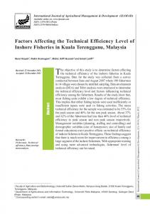
Fig. 1. Classical (crosses) and quantum (solid lines) probability distributions for walks on a line after 100 timesteps. Only even positions are shown since odd positions are zero. The classical walk is averaged over 50,000 iterations of the random walk. A skewed quantum walk is shown with an initial √0i along with a√symmetric quantum √ state of |0, walk with an initial state of either 0.15|0, 0i + 0.85|0, 1i or 1/ 2(|0, 0i + i|0, 1i).

as shown in eq. (3), which causes some probabilities to be amplified or decreased at each timestep. This leads to the different behaviour compared to its classical counterpart: spreading at a rate proportional to t, quadratically faster than the classical random walk. √ √ In addition, the centre part of the distribution, in the interval [−t/ 2, t/ 2], is fairly uniform. This is the opposite of the classical random walk which has an exponential drop in probability after just a few standard deviations from the origin. These properties of the quantum walk on the line were obtained by both Ambainis et al. [Ambainis et al. 2001] and Nayak and Vishwanath [Nayak and Vishwanath 2000]. As the walker can now be in a superposition of positions on the line, we obtain a probability distribution of the quantum walker after one run of the entire walk. Obviously, this is due to the fact the coin operator is now deterministic. However, if we were to measure the coin after the required number of timesteps, we would get a random output as in the classical case. We show both the classical and quantum probability distributions after 100 steps in fig. 1. If the walk is imperfect and some decoherence is allowed, we can see the gradual change from the quantum case back to classical. Kendon et al. [Kendon and Tregenna 2003] investigated this in detail showing that as the decoherence in the system grows, the spread of the walk gradually changes from the quantum walk shown above back to the classical binomial distribution. In the interim, we see a gradual change with an almost ‘top-hat’ distribution being found which is useful for random sampling. For a review of the effects of decoherence in quantum walks, see Kendon [Kendon 2007].


7

−3

x 10 8

6

Probability

Probability

0.3 0.25

4

2

0.2 0.15 0.1 0.05

0 50

0 50

40

40

30

50 30

20 10 50

Lattice length

40

30

20 45

40

35

30

25

20

15

10

5

10 Lattice width

Lattice width

20 10 Lattice length

Fig. 2. Dynamics of the quantum walk on a two dimensional Cartesian lattice using the Grover coin, eq. (5). LHS: Maximum spreading obtained using the initial state in eq. (7). RHS: Localisation obtained using the initial state in eq. (6). Note the different scales.

2.2. Discrete time quantum walk in higher dimensions We can see that the quantum walk exhibits interesting and very different behaviour to the classical walk even on the line. However, many interesting problems in computer science are defined in higher dimensions. In order to define the walk in these higher dimensional, we require a new coin operator, of dimension d, in order to span the entire coin state space of the walker [Moore and Russell 2002, Mackay et al. 2002, Kendon 2003, Kempe 2003]. This can be any unitary operator of the required dimension. Clearly many different possibilities exist but we only mention the most common operator here - the Grover coin,   2 . . . d2 d   (4) G(d) =  ... . . . ...  − Id , 2 2 ... d d where d is the degree of the vertex and Id is the identity operator of the same dimension. The Grover coin is symmetric but only balanced, i.e. it treats all directions in the same way - up to a phase factor, for the cases where d = 2 and d = 4. In the case of d = 3 and all higher dimensions, the coin treats one edge differently to the remaining d − 1. In addition to the coin operator, the conditional shift operator must also be modified. In the case of the line, it is easy to define as there are only two possible directions the walker can move in. In higher dimensions, the walker can move in any one of d directions. Kendon [Kendon 2003] treats this problem rigorously, but the most important thing is to maintain a consistent labelling approach for each of the edges. The dynamics of the walk on higher dimensional structures has been studied briefly by Mackay et al. [Mackay et al. 2002] and then in more detail by Tregenna et al. [Tregenna et al. 2003]. They numerically studied the spreading of the quantum walk with varying coin operators and initial states. Tregenna et al. found that the initial state of the walker on the lattice had a large impact on the spreading of the walker. Depending on the initial state, the walker can spread anywhere from a minimum possible spread to a maximum possible spreading (as defined in [Tregenna et al. 2003] by the second moment). Using the Grover


8

coin on a two dimensional Cartesian lattice, d = 4,  −1 1 1 1  1 1 −1 1 1 G(4) =  1 −1 1 2 1 1 1 1 −1



 , 

(5)

most of the initial states, including the symmetric initial state, |ψisym =

1 (|0, Li + i|0, Ri + |0, Di + i|0, U i) , 2

(6)

where L, R, D, U are the four directions the walker is able to move on the lattice, give a minimal spreading with the walker localising around the origin with high probability as seen in fig. 2. However, one specific state, |ψimax =

1 (|0, Li − |0, Ri + |0, Di − |0, U i) , 2

(7)

gives a maximal spreading, again shown in fig. 2. Inui et al. [Inui Konishi and Konno 2004] proved this localisation analytically for two dimensional lattices. In addition to these results, some analytical results have been shown for d-dimensional lattices. Grimmett et al. [Grimmett Janson and Scudo 2004] proved that in the limit n → ∞, Xn /n converges weakly where Xn is the position at time n in the case of the infinite line. Gottlieb et al. [Gottlieb 2005] later extended this result to show convergence on d-dimensional lattices.

2.3. The discrete time quantum walk search algorithm We now describe how Shenvi, Kempe and Whaley [Shenvi Kempe and Whaley 2003] were able to modify the quantum walk into a search algorithm. In their work, they analysed the search algorithm on a hypercube. Here, we show how the quantum walk search algorithm is applied to a 2D Cartesian lattice. The data points we wish to search are laid out as the vertices of an undirected graph. The edges then represent the specific connections between data points. At the edges of the lattice we impose periodic boundary conditions, in effect turning the graph into a torus. Our aim is to find one data item, a specific vertex, out of the set of data to be searched. We start the walker in an equal superposition of all the possible sites in the lattice, and the coin in an equal superposition of all directions, N d 1 XX |x, ci, |ψi = √ dN x=1 c=1

(8)

where d is the degree of the vertices in the graph and N is the total number of vertices. If we let the walker evolve in a natural fashion, using the Grover coin eq. (4), we would find a flat distribution identical to the starting state at any point in time. This uniform distribution is an eigenstate of the Grover coin operator. We need to use a different coin operator for the marked state in order to introduce a bias into the walk. It is optimal to invert the phase of the G(4) coin operator from eq. (5), as shown in [Lovett et al. 2011],


0.25

0.25 0.2 Probability

Probability

0.2 0.15 0.1 0.05

0.15 0.1 0.05

0 20

0 20 20

15

0

Lattice width

10

5

5 0

15

10

10

5

20

15

15

10

0

Lattice width

Lattice length

0.25

5 0

Lattice length

0.25 0.2 Probability

0.2 Probability

9

0.15 0.1 0.05

0.15 0.1 0.05

0 20

0 20 20

15 15

10 Lattice width

0

20

15 10

5

5 0

15

10

10

5

Lattice width

Lattice length

0

5 0

Lattice length

Fig. 3. Probability distribution of a discrete time quantum walk search on 400 vertices arranged in a 20 × 20 square with periodic boundary conditions, evolved for 0, 10, 20 and 32 timesteps. The marked vertex is at position 190. giving G(4) m

1 −1 1 −1 1 =  2  −1 −1 −1 −1 

 −1 −1 −1 −1  . 1 −1  −1 1

(9)

Figure 3 shows how the distribution of the walker evolves with time for a 20×20 lattice, i.e. N = 400. We see that using a different coin creates a defect in the walk and the probability coalesces on the marked state over time. As the walk progresses, the probability at the marked state cannot keep increasing without limit. In fact, we see in fig. 4 that the probability at the√marked state has periodic behaviour with the first peak occuring at roughly t = (π/2) N ≃ 32, with maximum probability for N = 400 of around 0.23. This can be increased as close to 1 as desired by standard amplification techniques (repeating the search a few times). We see √ that subsequent peaks occur at other integer multiples of this initial time, t = n(π/2) N where n = 2, 3, 4...... As we have now shown how the quantum walk can be turned into a search algorithm, we are interested in how quickly the quantum walker finds the marked state. That is, we want to know when the probability of the walker being present at the marked state is at a maximum. As this probability is periodic and we want the algorithm to be efficient, the subsequent peaks are not of interest: we want to know when the first peak occurs. Although it would be ideal to measure the walker at the precise timing of the maximum in the first peak, this is not strictly necessary. In fact, as can be seen in fig. 4, the peaks are quite broad, so even if an error occurs in when to measure, it only means a somewhat lower probability of finding the marked state, this is only a constant extra overhead on the amplification. For example, if the state of the walker was measured at half the optimal


10

0.25

Probability of marked state

0.2

0.15

0.1

0.05

0 0

20

40

60

80

100 Timestep

120

140

160

180

200

Fig. 4. Probability of the marked state over 200 timesteps on a 20 × 20 grid with periodic boundary conditions. The marked vertex is at position 190. √ number of timesteps (t = (π/4) N ≃ 16), the probability of the walker being measured in the marked state is roughly half that of the maximum possible (p ≈ 0.1). In later sections, we discuss the algorithmic efficiency of the search algorithm on various graph structures. It is important we define here what factors of efficiency we are interested in. As we are looking to find a specific item from a set of many, we must consider how likely it is the walker coalesces at the marked state. The maximum probability of the walker at the marked state, i.e. the maximum value of the first peak, varies with the size of the dataset (for the 2D Cartesian lattice). In this case, the theoretical value of O(1/ log2 N ) from Ambainis [Ambainis 2003] is numerically confirmed in our results in fig. 5 with a small prefactor of just over 2. The second factor we are interested in is the number of timesteps it takes to reach this maximum probability. The scaling of the time to find the marked state with the size √ of the dataset, N , for the 2D Cartesian lattice is shown in fig. 6. We see a scaling of O( N ) here, also with a prefactor of 2. In order to compare our results in later chapters to previous work, we must consider the total algorithmic complexity of the quantum walk search algorithm. In the case of the 2D Cartesian lattice, the maximum probability scales as O(1/ log2 N ). Hence, we must use amplitude amplification techniques to increase this to a constant value. This √ has previously been shown to take O( log N ) time steps [Brassard 2002]. This makes √ the total algorithmic complexity O( N log N ) for the 2D lattice, in agreement with the recent results of Tulsi [Tulsi 2008] and Magniez et al. [Magniez et al. 2009]. These scalings are not the same for all graph structures. In particular, on a cubic lattice, the maximum probability scales as a constant value O(1). As such, only a constant number of amplification steps are √needed to bring the probability to ≈ 1, thus the total algorithmic complexity is just O( N ).

3. Dimensionality In this section, we investigate how the spatial dimension of the database arrangement affects the searching algorithm. We already know, as noted in sec. 2, that the basic


11

Maximum probability of marked state

0.5 2D Cartesian lattice 2.173/log2 N 0.4

0.3

0.2

0.1

0 0

0.5

1

1.5

2

2.5 3 Vertices (N)

3.5

4

4.5

5 4

x 10

Fig. 5. Maximum of the first peak in the probability of being at the marked state for different √ sized√data sets, using the optimal marked state coin in eq. (9) on a 2D lattice of size N × N , plotted against N (crosses). Also shown is the closest fit to our data, 2.173/ log2 N (dashes).

Timestep to first significant peak

500

2D Cartesian lattice 2 sqrt(N)

400

300

200

100

0 0

50

100 150 Length of lattice (sqrt(N))

200

Fig. 6. Time step at which the first peak in the probability of being at the marked state occurs for different√sized data sets, using the optimal marked state√coin in eq. (9), plotted against N . Also shown is the closest fit to our data, 2 N .

scaling of the algorithm is heavily dependent upon the spatial dimension of the structure in question. Both the scaling of the maximum probability of the marked state and the time to find this probability alter for structures of differing spatial dimension. We are interested here in how this basic scaling changes when the spatial dimension is altered. We investigate this in two ways: firstly by introducing a simple form of tunnelling, which allows us to interpolate between structures of varying spatial dimension, and secondly by using lattices of varying height (1D-2D) and depth (2D-3D).


12

Fig. 7. Basic unit of the structure we use to interpolate between the two dimensional Cartesian and the three dimensional cubic lattices. The solid lines represent the fixed, normal edges whereas the dashed lines represent the edges we set to be tunnelling. 3.1. Tunnelling operator We now describe a modified coin operator we will use in the search algorithm to gradually vary the connectivity of the structures studied. We introduce a simple form of tunnelling to allow us to gradually vary the substrate to be walked upon from one form to another. A simple example is changing a set of 2D Cartesian lattices into a cubic lattice by introducing connecting links between the lattices, see fig. 7. In order to achieve the quantum walk dynamics we require, we must use a different coin operator. The only condition on this operator is that it must be unitary. As such, we ‘design’ a new coin operator which incorporates a single tunnelling parameter, c, which will allow us to vary the strength of specific tunnelling edges. We define d to be the degree of the vertex in question as used previously in the Grover coin, eq. (4), and t to be the number of tunnelling edges. For a d-dimensional vertex, the first (d−t) edges in our labelling scheme are normal and the last t edges are tunnelling. In fig. 7, the solid edges are normal, fixed edges creating a 2D lattice and the dashed edges are tunnelling edges which convert the 2D lattices to a cubic one. The general matrix for the desired coin operator would be as follows:   a b b ... b c c c ... c  b a b ... b c c c ... c       . . . ... . . . . ... .     . . . ... . . . . ... .     . . . ... . . . . ... .     b b b ... a c c c ... c   Td,t =  (10)  c c c ... c e f f ... f     c c c ... c f e f ... f       . . . ... . . . . ... .     . . . ... . . . . ... .     . . . ... . . . . ... .  c c c ... c f f f ... e where the blocks of “abbb...” are d − t square and the blocks of “ef f f...” are t square. We want to be able to rewrite this in terms of just one tunnelling parameter, c, which represents the coupling between the normal and tunnelling edges. As the dynamics of


13

the walk must be reversible, we must ensure that the coin produced is unitary. As such, †

(Td,t ) (Td,t ) = Id ,

(11)

†

must hold, where (Td,t ) is the hermitian conjugate of the general matrix. We can solve the five equations which are formed as a consequence in terms of just the degree of the lattice, d, the number of tunnelling edges, t and the tunnelling parameter, c, giving a = b − 1, p 1 + 1 − (d − t)tc2 , b= d−t

(12) (13)

e = f − 1,

and

(14)

p 1 − (d − t)tc2 f= . (15) t This operator allows us to vary the ‘strength’ of certain edges in the structure we wish to walk on. It holds for any degree of vertex but the number of tunnelling edges must be at most half the degree, i.e. t ≤ d/2. By using vertices of degree six with two tunnelling edges, we have a set of basic 2D Cartesian lattices gradually becoming a cubic lattice as in fig. 7. In this case, setting c = 0 we obtain   −1 1 1 1 0 0  1 −1 1 1 0 0      1 1 1 −1 1 0 0  (16) T6,2 =  , 1 1 −1 0 0  2 1    0 0 0 0 −2 0  0 0 0 0 0 −2 1−

and setting c = 2/d = 1/3 gives  T6,2

  1  =  3  

−2 1 1 −2 1 1 1 1 1 1 1 1

1 1 1 1 1 1 1 1 −2 1 1 1 1 −2 1 1 1 1 −2 1 1 1 1 −2



    .   

(17)

These choices of c represent the extremes of the operator when the structure would be either a basic 2D Cartesian lattice, eq. (16), or a cubic lattice, eq. (17). Any other values of c where 0 ≤ c ≤ 2/d would give varying strengths of tunnelling across the tunnelling edges. 3.2. Interpolating between the 2D and 3D lattices using the tunnelling operator Using the tunnelling operator introduced above, we numerically study how the algorithm is affected by the change in spatial dimension. We use the operator to interpolate between a Cartesian lattice (2D) and a cubic lattice (3D). In this case, we interpolate between


14

a set of 2D Cartesian lattices and a fully connected cubic lattices by using vertices of degree six with two tunnelling edges, with the correct connectivity, fig. 7. Although we do not show the results here, we also performed the same investigation between the 1D line and the 2D lattice, finding a quantitatively similar result. The results in this case were more difficult to analyse due to the search algorithm failing as the structure approached a line. The search algorithm we use is the same as in the original work by Shenvi, Kempe and Whaley [Shenvi Kempe and Whaley 2003], with a small change to the initial state. Although we must still start the walker in a uniform superposition over all vertices, the distribution over the edges must be altered slightly to account for the strength of the tunnelling edges. In other words, we must distribute the state over the edges with a weighting to match the tunnelling strength as follows 1 (d − t)α + tpα = √ , N

(18)

where p is the tunnelling probability, α is the state on each edge and N is the number of vertices. The tunnelling probability is just the tunnelling parameter, c, rescaled to lie between 0 and 2/d. In this way, the tunnelling probability matches the proportion of the initial state which is placed on the tunnelling edges. This initial state gives a probability distribution, where there is no marked state, which is periodic over two timesteps as can easily be checked. Although this is not stationary as in the case of the basic nontunnelling lattices, the fact that it returns to the same state after only two timesteps means it will give rise to the same dynamics. We ran the algorithm on a 3D cubic lattice where the edges which link the ‘slices’ of 2D lattices together are tunnelling. We show the a basic unit in fig. 7. The solid lines are the fixed, normal edges and the dashed lines are tunnelling edges. This structure allows us to gradually change the strength of the edges which make the structure three dimensional, hence interpolating between the 2D Cartesian lattice and the 3D cubic lattice. The maximum probability of the marked state, shown in fig. 8, changes from the 1/ log2 N scaling in the 2D case to the constant O(1) scaling as soon as the additional edges even have a small weighting attached to them. At low tunnelling strengths, we see the probability dropping initially before gradually recovering towards a constant value for higher lattice sizes. At these higher sizes, it is easy to see that the scaling is constant for any tunnelling strength with just varying prefactors. Figure 9 shows how this prefactor to the scaling of the maximum probability of the marked state changes as we increase the tunnelling probability. The sharp drop at the low tunnelling probabilities is most probably due to the fact the scaling hasn’t reached the constant value as we can only simulate up to a fixed lattice size. In addition, we note here that when the probability of tunnelling is zero, the scaling does not match that of the basic 2D lattice. At p = 0, the structure is in effect a collection of 2D lattices which are unlinked. The initial state is still spread across all these individual lattices and due to the connectivity of the structure, only the amplitude in one of the lattices (that with the marked state present) is able to coalesce on the marked state. As such, the scaling is just reduced by a constant factor as can be seen in fig. 8.


15

0.5

3D Lattice 2D Lattice p=0 p = 0.1 p = 0.2 p = 0.3 p = 0.4 p = 0.5 p = 0.6 p = 0.7 p = 0.8 p = 0.9 p=1


0.45 0.4 0.35 0.3 0.25 0.2 0.15 0.1 0.05 0 0

1

2

3 Vertices (N)

4

5

6 4

x 10

Prefactor to the scaling of the maximum probability of the marked state

Fig. 8. Plot to show how the maximum probability of the marked state varies with both the size of the lattice and the tunnelling strength as a two dimensional lattice is gradually changed into a three dimensional Cartesian lattice. 0.35

0.3

0.25

0.2

0.15

0.1

0.05

0 0

0.1

0.2

0.3

0.4 0.5 0.6 Tunnelling probability

0.7

0.8

0.9

1

Fig. 9. Plot to show how the prefactor to the scaling of the maximum probability of the marked state, obtained from the data in fig. 8, varies with the tunnelling strength as a two dimensional Cartesian lattice is gradually changed into a three dimensional lattice. The time to find the marked state follows a similar behaviour. We firstly show, fig. 10, how the scaling of the time to find the marked state varies with both the size of the lattice and the tunnelling strength. The basic scaling √ of the time to find the marked state is the same in both two and three dimensions, O( N ). We see that, in general, the time to find the marked state (the prefactor to the basic scaling) decreases as the tunnelling strength increases, thus making the algorithm more efficient. We show a plot of how this prefactor varies with the tunnelling strength in fig. 11. We do note that at the very low tunnelling probabilities, p 0.65. Below this probability, the quantum speed up disappears gradually to end at the classical run time when p = pc . This is for the same reason as in the scaling of the maximum probability of the marked state, at the critical threshold the structure is effectively a line. Below the critical threshold, the algorithm fails (the marked state is probably in a disconnected region). We note here that the coefficient, α, is not exactly 0.5 as we expect for the quadratic speed up. This is most probably due to the fact that percolation lattices are random in nature, and we only average over a specific number. If we averaged over more, then we would see a more constant scaling of the coefficient at α = 0.5, i.e. a full quadratic speed up. 5.4. Three dimensional percolation lattices We now turn our attention to three dimensional site percolation lattices. We follow the same analysis as in the two dimensional case. We firstly show, fig. 31, how the maximum probability of the marked state varies as the percolation probability is decreased. We see, as in the two dimensional case, that the basic scaling of the maximum probability matches that of the three dimensional lattice until the percolation probability drops to roughly the critical percolation threshold, pc = 0.3116.... We show in fig. 32, how the prefactor to this scaling of the maximum probability varies with the percolation probability. In the same way as the two dimensional case, we see an almost linear scaling of the prefactor once the percolation probability has passed the critical threshold. The scaling here doesn’t seem to be as close as in the two dimensional case. This is probably because in the case of three dimensional percolation lattices, there are many more combinations of lattice which can be created. Averaging over more of these lattices would most probably give a smoother fit. The time to find the marked state, in the three dimensional case, follows the same behaviour as in the two dimensional percolation lattices. We show in fig. 33, how the time to find the marked state varies with the percolation probability. We see, fig. 34, as in the two dimensional case, that the scaling coefficient, α, gradually changes from the quadratic speed up to the classical run time. Again, we note that the quadratic speed


31

0.5

3D lattice p = 0.95 p = 0.9 p = 0.85 p = 0.8 p = 0.75 p = 0.7 p = 0.65 p = 0.6 p = 0.55 p = 0.5 p = 0.45 p = 0.4 p = 0.35 p = 0.3 p = 0.2


0.45 0.4 0.35 0.3 0.25 0.2 0.15 0.1 0.05 0 0

500

1000

1500 2000 Square root of vertices

2500

3000

Prefactor to scaling of maximum probability of marked state

Fig. 31. Plot to show how the maximum probability of the marked state varies with the percolation probability in three dimensions. We also show the same plot for a fully connected three dimension lattice (dashed line). 0.4

0.35 0.3

0.25 0.2

0.15 0.1

0.05 0 0.2

0.3

0.4

0.5

0.6 0.7 Percolation probability

0.8

0.9

1

Fig. 32. Plot to show how the prefactor to the scaling of the maximum probability of the marked state, from the data in fig. 31, varies with the size of the dataset and the percolation probability for site percolation in three dimensions. up is maintained for a non-trivial amount of disorder before gradually changing to the classical run time at the point p = pc . We do note, as in the two dimensional case, that the coefficient is not exactly 0.5. This can be explained in the same way as the two dimensional percolation lattices, and averaging over more lattices should give a constant value of the coefficient α. 6. Discussion In this paper, we have discussed various factors which affect the efficiency of the quantum walk search algorithm. We introduce a simple form of tunnelling which allows us to modify the substrate we use as the database arrangement, and use this to interpolate between structures with varying dimensionality and degree. We find that although the dependence


32

1000

3D lattice p = 0.95 p = 0.9 p = 0.85 p = 0.8 p = 0.75 p = 0.7 p = 0.65 p = 0.6 p = 0.55 p = 0.5 p = 0.45 p = 0.4 p = 0.35 p = 0.3 p = 0.2 O(N)

Timestep to first significant peak

900 800 700 600 500 400 300 200 100 0

10

15

20

25

30 35 40 Square root of vertices

45

50

55

60

Scaling of the exponent of the time to find the marked state

Fig. 33. Plot to show how the time to find the marked state varies with the size of the dataset and the percolation probability for site percolation lattices in three dimensions. We also show the same plot for a fully connected three dimension lattice (dashed line).

2.2 2.1 2 1.9 1.8 1.7 1.6 1.5 1.4 1.3 1.2 1.1 1 0.9 0.8 0.7 0.6 0.5 0.4 0.2

3D percolation lattices α = 0.5

0.3

0.4

0.5 0.6 0.7 Percolation probability

0.8

0.9

1

Fig. 34. Plot to show how the exponent, α, to the scaling of the time to find the maximum probability of the marked state, from the data in fig. 33, varies with the size of the dataset and the percolation probability for site percolation in three dimensions. Also shown is α = 0.5 to indicate the lower bound of the algorithm (dashed line).

on the spatial dimension of the underlying substrate is strong, it is not the only factor which affects the efficiency of the algorithm. We also find secondary dependencies on the connectivity and symmetry of the structure. In addition, we use percolation lattices to model disorder in the lattice in a simple way. In this case we find, counter-intuitively, that the algorithm is able to maintain the quantum speed up even in the presence of non trivial levels of disorder. We now discuss our findings for each factor in turn.


33

6.1. Dimensional dependence We have shown two different ways in which we can interpolate between structures of differing spatial dimension. Firstly, we use a tunnelling operator to vary specific edges of a lattice enabling us to gradually change the spatial dimension of the lattice. In this case, we find a sudden change in the scaling of the maximum probability of the marked state as soon as there is even a very small probability of the edges existing. This seems to indicate that the ‘strength’ of the edges in the lattice is of little importance, with the dependence on the specific spatial dimension taking precedence. However, we find that the prefactor to the scaling of this probability varies with the strength of the tunnelling edges, increasing as the tunnelling strength increases. The basic scaling of the time to find the marked state is not affected by the change in dimensionality, we note though that the prefactor to the scaling decreases as the tunnelling strength increases, hence the algorithm becomes more efficient. The other case we consider is the case of lattices with varying height or depth, for example, a 3D lattice with fixed width and height but of varying depth. Although this structure is still strictly three dimensional, when the depth is very low and the width (height) is large, the quantum walker will see the structure as almost a basic 2D Cartesian lattice. Suprisingly, in this case we see a gradual change in scaling in the maximum probability of the marked state. At low depths of the lattice, the scaling is almost the same as the lower spatial dimensional structure gradually changing to the higher dimensional structure scaling as the depth increases to become equal to that of the other dimensions. This highlights the importance of full symmetry in the quantum walk search algorithm.

6.2. Connectivity We show how the search algorithm is affected by varying connectivity in regular lattices. We use our simple model of tunnelling to allow us to interpolate between structures such as the square lattice (d = 4) and the triangular lattice (d = 6). With this model, we are able to identify how the prefactors to the scaling of both the maximum probability of the marked state and the time to find the marked state vary with the connectivity of the structure. √ The basic scaling of the time to find the marked state, O( N ), is not affected by the increase in connectivity but we find the prefactor to this scaling reduces as the connectivity of the structure being searched increases. This is due to the additional paths the walker can take to coalesce on the marked state, thus increasing the efficiency of the algorithm in both two and three dimensions. The maximum probability of the marked state is also affected by the connectivity of the underlying structure. We find that the additional connectivity does not affect the basic scaling of O(1/ log2 N ) in the two dimensional case. Only moving to three spatial dimensions allows the walker to find the marked state with a constant probability, O(1). However, we do note that in both two and three dimensions the prefactors to this scaling, in general, increase as the connectivity of the structure increases. Again, this increases the efficiency of the algorithm as it may not have to be repeated so many


34

times. We also find that the probability of the marked state does not increase uniformly with the additional connectivity. We see the prefactor in the scaling drop and then recover itself before increasing as the tunnelling strength increases. This is due to the dynamics of the quantum walk on a structure with some broken symmetry, i.e. low tunnelling strength between vertices. We briefly investigated the dynamics of the walk by starting the walker in a single location and monitoring how quickly it spread outwards with varying tunnelling strengths. This confirmed our results for the search algorithm as we found that the spread of the quantum walk also dropped for lower tunnelling strengths before recovering and eventually increasing at higher tunnelling probabilities. However, this work on the spreading of the walk compared to tunnelling strength is by no means exhaustive and it would be interesting to look more deeply into this in the future. 6.3. Substrate disorder We studied both two and three dimensional percolation lattices as a way to model disorder in the quantum walk search algorithm. We are interested in how the algorithm performs with increasing disorder. We use percolation lattices as a random substrate for the database arrangement we wish to search. We find, in both the two and three dimensional cases, that as the level of disorder increases, the maximum probability of the marked state decreases. Whilst the percolation probability is higher than the critical percolation threshold, the basic scaling of the maximum probability of the marked state matches that of the basic lattice (in that spatial dimension). Once the percolation probability drop to the critical threshold, this scaling changes to that of the line, 1/N . This is expected as at this point the structure is effectively a line. We also note the prefactor to the scaling of the maximum probability of the marked state increases linearly once the percolation probability is greater than the critical threshold. The time to find the marked state follows a similar behaviour. We find that as the disorder increases, the time to find the marked state also increases. Surprisingly though, we note that the quadratic speed up is maintained for a non-trivial level of disorder, before gradually reverting to the classical run time, O(N ), as the disorder reaches the critical percolation threshold. This seems to match the results of [Leung et al. 2010], which show a fractional scaling for the spreading of the quantum walk from a maximal quantum spreading to a classical spreading at and below the critical threshold. However, this is in contrast to the work of Krovi and Brun [Krovi and Brun 2006, Krovi and Brun 2006, Krovi and Brun 2007] who highlight the effect of localisation on the quantum walk when defects are introduced into the substrate. Both these factors indicate that the quantum walk search algorithm seems to be more robust to the effects of disorder and symmetry than the basic spreading of the quantum walk. This could be due to the fact that the initial state of the walker is spread across the whole lattice. We have seen that the algorithm becomes less efficient as the disorder increases, but at percolation probabilities greater than the critical threshold, the algorithm still seems to be viable, although more amplification of the result may be required.


35

Acknowledgments The authors would like to thank Jiannis Pachos and Noah Linden for useful and interesting discussions. NL was funded by the UK Engineering and Physical Sciences Research Council. VK is funded by a UK Royal Society University Research Fellowship.

References S. Aaronson and A. Ambainis. Quantum search of spatial regions. In Proceedings of the 44th annual IEEE symposium on foundations of computer science (FOCS), 2003, pages 200–209. IEEE, 2003. G. Abal, R. Donangelo, F. L. Marquezino, A. C. Oliveira, and R. Portugal. Decoherence in Search Algorithms. Proceedings of the 29th Brazilian computer society congress (SEMISH), pages 293–306, 2009. G. Abal, R. Donangelo, F. L. Marquezino, and R. Portugal. Spatial search in a honeycomb network. To appear in Mathematical Structures in Computer Science. Arxiv preprint arXiv:1001.1139, 2010. D. Aharonov, A. Ambainis, J. Kempe, and U. Vazirani. Quantum walks on graphs. In Proceedings of the 33rd annual ACM symposium on theory of computing (STOC), pages 50–59. ACM, 2001. A. Ambainis. Quantum walks and their algorithmic applications. International Journal of Quantum Information, 1:507–518, 2003. A. Ambainis. Quantum walk algorithm for element distinctness. In Proceedings of the 45th annual IEEE symposium on foundations of computer science (FOCS), 2004, pages 22–31. IEEE, 2004. A. Ambainis, E. Bach, A. Nayak, A. Vishwanath, and J. Watrous. One-dimensional quantum walks. In Proceedings of the 33rd annual ACM symposium on theory of computing (STOC), pages 37–49. ACM, 2001. A. Ambainis, J. Kempe, and A. Rivosh. Coins make quantum walks faster. In Proceedings of the 16th annual ACM-SIAM symposium on discrete algorithms (SODA), pages 1099– 1108. Society for Industrial and Applied Mathematics, 2005. P. Benioff. Space searches with a quantum robot. Quantum Computation and Information, 305:1, 2002. E. Bernstein, C. Bennett, G. Brassard, and U. Vazirani. Strengths and weaknesses of quantum computing. SIAM Journal of Computing, 26:1510–1523, 1997. G. Brassard, P. Høyer, M. Mosca, and A. Tapp. Quantum amplitude amplification and estimation. In Quantum Computation and Information, volume 305, pages 53–74. American Mathematical Society, Providence, RI., 2002. H. Buhrman and R. Spalek. Quantum verification of matrix products. Proceedings of the 17th annual ACM-SIAM symposium on discrete algorithms, 2004, 2004. A. M. Childs. Universal computation by quantum walk. Physical Review Letters, 102:180501, 2009. A. M. Childs and J. Goldstone. Spatial search and the Dirac equation. Physical Review A, 70:42312, 2004.


36

A. M. Childs and J. Goldstone. Spatial search by quantum walk. Physical Review A, 70:22314, 2004. Z. V. Djordjevic, H. E. Stanley, and A. Margolina. Site percolation threshold for honeycomb and square lattices. Journal of Physics A: Mathematical and General, 15:L405, 1982. E. Farhi and S. Gutmann. Quantum computation and decision trees. Physical Review A, 58:915–928, 1998. T. Gebele. Site percolation threshold for square lattice. Journal of Physics A: Mathematical and General, 17:L51, 1984. A. D. Gottlieb. Convergence of continuous-time quantum walks on the line. Physical Review E, 72:47102, 2005. G. Grimmett, S. Janson, and P. F. Scudo. Weak limits for quantum random walks. Physical Review E, 69:26119, 2004. L. K. Grover. A fast quantum mechanical algorithm for database search. Proceedings of the 28th annual ACM symposium on theory of computing (STOC), 1996, page 212, 1996. B. Hein and G. Tanner. Quantum search algorithms on the hypercube. Journal of Physics A: Mathematical and Theoretical, 42:085303, 2009. B. Hein and G. Tanner. Quantum search algorithms on a regular lattice. Physical Review A, 82:12326, 2010. N. Inui, Y. Konishi, and N. Konno. Localization of two-dimensional quantum walks. Physical Review A, 69(5):052323, 2004. J. P. Keating, N. Linden, J. C. F Matthews, and A. Winter. Localization and its consequences for quantum walk algorithms and quantum communication. Physical Review A, 76:12315, 2007. J. Kempe. Quantum random walks: an introductory overview. Contemporary Physics, 44:307–327, 2003. J. Kempe. Quantum random walks hit exponentially faster. In Lecture Notes in Computer Science - Proceedings of RANDOM’03, volume 2764, pages 354–369. Springer, 2003. V. Kendon. Quantum walks on general graphs. International Journal of Quantum Information, 4:791, 2003. V. Kendon. Decoherence in quantum walks - a review. Mathematical Structures in Computer Science, 17:1169–1220, 2007. V. Kendon and B. Tregenna. Decoherence can be useful in quantum walks. Physical Review A, 67:42315, 2003. H. Krovi and T. A. Brun. Hitting time for quantum walks on the hypercube. Physical Review A, 73:32341, 2006. H. Krovi and T. A. Brun. Quantum walks with infinite hitting times. Physical Review A, 74:42334, 2006. H. Krovi and T. A. Brun. Quantum walks on quotient graphs. Physical Review A, 75:62332, 2007. H. Krovi, F. Magniez, M. Ozols, and J. Roland. Finding is as easy as detecting for quantum walks. Automata, Languages and Programming, pages 540–551, 2010.


37

G. Leung, P. Knott, J. Bailey, and V. Kendon. Coined quantum walks on percolation graphs. New Journal of Physics, 12:123018, 2010. N. B. Lovett, S. Cooper, M. Everitt, M. Trevers, and V. Kendon. Universal quantum computation using the discrete-time quantum walk. Physical Review A, 81:42330, 2010. Neil Lovett, Matthew Everitt, Matthew Trevers, Daniel Mosby, Dan Stockton, and Viv Kendon. Spatial search using the discrete time quantum walk. Natural Computing, pages 1–13, 2011. 10.1007/s11047-011-9279-4. T. D. Mackay, S. D. Bartlett, L. T. Stephenson, and B. C. Sanders. Quantum walks in higher dimensions. Journal of Physics A: Mathematical and General, 35:2745, 2002. F. Magniez and A. Nayak. Quantum complexity of testing group commutativity. Automata, Languages and Programming, pages 1312–1324, 2005. F. Magniez, A. Nayak, P. C. Richter, and M. Santha. On the hitting times of quantum versus random walks. In Proceedings of the 20th annual ACM-SIAM symposium on discrete algorithms (SODA), pages 86–95. Society for Industrial and Applied Mathematics, 2009. F. Magniez, A. Nayak, J. Roland, and M. Santha. Search via quantum walk. In Proceedings of the 39th annual ACM symposium on theory of computing (STOC), pages 575–584. ACM, 2007. F. Magniez, M. Santha, and M. Szegedy. Quantum algorithms for the triangle problem. In Proceedings of the 16th annual ACM-SIAM symposium on discrete algorithms (SODA), pages 1109–1117. Society for Industrial and Applied Mathematics, 2005. F. L. Marquezino, R. Portugal, and G. Abal. Mixing Times in Quantum Walks on Two-Dimensional Grids. Physical Review A, 82:042341, 2010. C. Moore and A. Russell. Quantum walks on the hypercube. Proceedings of 6th international workshop on randomization and approximation techniques in computer science (RANDOM), pages 164–178, 2002. A. Nayak and A. Vishwanath. Quantum walk on the line. DIMACS Technical Report 2000-43, Arxiv preprint arXiv:0010117, 2000. A. Patel, K. S. Raghunathan, and Md. A. Rahaman. Search on a Hypercubic Lattice through a Quantum Random Walk: II. d=2. Physical Review A, 82:032331, 2010. A. Patel and Md. A. Rahaman. Search on a Hypercubic Lattice through a Quantum Random Walk: I. d¿2. Physical Review A, 82:032330, 2010. V. Potoˇcek, A. G´ abris, T. Kiss, and I. Jex. Optimized quantum random-walk search algorithms on the hypercube. Physical Review A, 79:12325, 2009. D. Reitzner, M. Hillery, E. Feldman, and V. Buˇzek. Quantum searches on highly symmetric graphs. Physical Review A, 79:12323, 2009. M. Santha. Quantum walk based search algorithms. Theory and Applications of Models of Computation. Springer, 2008. 31–46. R. A. M. Santos and R. Portugal. Quantum Hitting Time on the Complete Graph. To appear in International Journal of Quantum Information. Arxiv preprint arXiv:0912.1217, 2009. N. Shenvi, J. Kempe, and K. B. Whaley. A quantum random-walk search algorithm. Physical Review A, 67:52307, 2003. D. Stauffer and A. Aharony. Introduction to percolation theory. Taylor & Francis, 1992.


38

M. Szegedy. Quantum Speed-Up of Markov Chain Based Algorithms. In Proceedings of 45th annual IEEE symposium on foundations of computer science (FOCS), pages 32–41. IEEE, 2004. B. Tregenna, W. Flanagan, R. Maile, and V. Kendon. Controlling discrete quantum walks: coins and initial states. New Journal of Physics, 5:83, 2003. A. Tulsi. Faster quantum-walk algorithm for the two-dimensional spatial search. Physical Review A, 78:12310, 2008. M. S. Underwood and D. L. Feder. Universal quantum computation by discontinuous quantum walk. Physical Review A, 82:042304, 2010. C. Zalka. Grover′s quantum searching algorithm is optimal. Physical Review A, 60:2746– 2751, 1999.