The R Package dti - Journal of Statistical Software

JSS

Journal of Statistical Software September 2009, Volume 31, Issue 9.

http://www.jstatsoft.org/

Structural Adaptive Smoothing in Diffusion Tensor Imaging: The R Package dti J¨ org Polzehl

Karsten Tabelow

WIAS, Berlin

WIAS and MATHEON, Berlin

Abstract Diffusion weighted imaging has become and will certainly continue to be an important tool in medical research and diagnostics. Data obtained with diffusion weighted imaging are characterized by a high noise level. Thus, estimation of quantities like anisotropy indices or the main diffusion direction may be significantly compromised by noise in clinical or neuroscience applications. Here, we present a new package dti for R, which provides functions for the analysis of diffusion weighted data within the diffusion tensor model. This includes smoothing by a recently proposed structural adaptive smoothing procedure based on the propagationseparation approach in the context of the widely used diffusion tensor model. We extend the procedure and show, how a correction for Rician bias can be incorporated. We use a heteroscedastic nonlinear regression model to estimate the diffusion tensor. The smoothing procedure naturally adapts to different structures of different size and thus avoids oversmoothing edges and fine structures. We illustrate the usage and capabilities of the package through some examples.

Keywords: structural adaptive smoothing, diffusion weighted imaging, diffusion tensor model, Rician bias, R.

1. Introduction The basic principles of magnetic resonance diffusion weighted imaging (DWI) were introduced in the 1980’s (LeBihan and Breton 1985; Merboldt, Hanicke, and Frahm 1985; Taylor and Bushell 1985), after nuclear magnetic resonance (NMR) had long been known to be sensitive to diffusion of molecules in complex systems (Carr and Purcell 1954). Since then, DWI has evolved into a versatile tool for in-vivo examination of tissues in the human brain (Le Bihan, Mangin, Poupon, Clark, Pappata, Molko, and Chabriat 2001) and spinal cord (Clark, Barker, and Tofts 1999). DWI probes microscopic structures well beyond typical image resolutions

2

dti: Structural Adaptive Smoothing in Diffusion Tensor Imaging

through water molecule displacement, a fact attracting broad interest in this technique. It can be used in particular to characterize the integrity of neuronal tissue in the central nervous system. NMR images are acquired from signals measured in k-space by fast Fourier transform. In the case of single receiver coil systems and additive complex Gaussian noise in k-space, referred to as thermal noise below, this results in image grey values that follow a Rician distribution Rice(θ, σ) (Rice 1945). This distribution is characterized by two parameters: θ, corresponding to the signal of interest, and σ related to the noise standard deviation in k-space. Diffusion in neuronal tissue depends on the particular microscopic structure of the tissue and is usually not isotropic. Different diffusion directions ~b can be probed by applying bipolar magnetic field diffusion gradients (Stejskal and Tanner 1965). Let S~b denote the acquired diffusion weighted image with the ”b-value” b, which depends on the pulse sequence parameters. The non-diffusion weighted image (b = 0) is denoted by S0 . Due to the diffusion of water molecules during the application of the magnetic field gradient, the signal S~b is attenuated relative to S0 : S~b ∼ Rice(θ0 exp(−bD(~b)), σ) , S0 ∼ Rice(θ0 , σ) (1) where D(~b) is the diffusion constant probed in direction ~b. Equation 1 imposes several problems for the data analysis. I. The model for the measured data S is nonlinear in D. II. The measured data S suffers from noise typical for NMR images. While for the non-diffusion weighted image S0 a Gaussian noise model seems to be an appropriate approximation, the Rician distribution of the attenuated signal values S~b can be significantly different from a Gaussian. Ignoring this introduces a bias into the estimation of the diffusion constant and hence all derived quantities. III. The lower the noise level in the measured data is, the more accurately the diffusion constant can be estimated. Thus, a noise reduction would be helpful to improve the accuracy of the diagnostic measures derived from the data. Typically, diffusion weighted images S~b are measured for up to 100 (or more) diffusion gradient directions ~b resulting in very high-dimensional data. It was the development of diffusion tensor imaging (DTI, Basser, Mattiello, and LeBihan 1994a,b), see also Mori (2007) for an introduction, which triggered a plethora of clinical and neuroscience applications of DWI. There, the high-dimensional information in the diffusion weighted images is reduced to a Gaussian distribution model for free anisotropic diffusion. Within this model, diffusion is completely characterized by a rank-2 diffusion tensor D, a symmetric positive definite 3 × 3 matrix with six independent components. This model describes diffusion completely if the microscopic diffusion properties within a voxel are homogeneous and non-restricted. In the presence of partial volume effects, like crossing fibers, this model is only an approximation. For these cases, more sophisticated models exist, which rely on the measurement of diffusion weighted images with high angular resolution (Tuch, Weisskoff, Belliveau, and Wedeen 1999; Frank 2001). These shall not be considered in this paper. Due to recording the image volumes sequentially in time the data acquisition process is prone to artifacts caused e.g., by head motion, respiration and heartbeat. Image registration is usually applied to reduce these effects. We refer to Brammer (2001); Lazar (2008) or Mori (2007) for an overview and to Eddy, Fitzgerald, and Noll (1996) or Cox and Jesmanowicz (1999) for more specific algorithms. For a comparison of software packages for registration see Oakes, Johnstone, Walsh, Greischar, Alexander, Fox, and Davidson (2005).

Journal of Statistical Software

3

DTI suffers from significant noise which may render subsequent analysis or medical decisions more difficult. Noise here summarizes several effects (Lazar 2008), e.g., thermal noise caused by thermal motion of electrons, physiological noise summarizing effects of the respiratory and cardiological cycles and system noise created by fluctuations within the MR hardware. Physiological noise can partly be controlled within the acquisition process (Hu, Le, Parrish, and Erhard 1995; Glover, Li, and Ress 2000). In the presence of thermal noise the estimation of anisotropy indices from the diffusion tensor is known to be systematically biased (Basser and Pajevic 2000; Hahn, Prigarin, Heim, and Hasan 2006). In addition to the common random errors the order of the diffusion eigenvectors of the tensor which is essential for fiber tracking is subject to a sorting bias especially at high noise levels. Noise reduction is therefore essential. Smoothing in tensor space, using log-Euclidian or Riemannian metrics and anisotropic or non-linear diffusion is e.g., proposed in Fletcher (2004); Pennec, Fillard, and Ayache (2006); Arsigny, Fillard, Pennec, and Ayache (2006); Fillard, Arsigny, Pennec, and Ayache (2007a) and Fletcher and Joshi (2007). In Tabelow, Polzehl, Spokoiny, and Voss (2008) we proposed a new smoothing method for noise reduction in DTI based on the propagation-separation (PS) approach (Polzehl and Spokoiny 2006). The procedure has been shown to naturally adapt to the structures of interest at different scales (Tabelow et al. 2008; Polzehl and Spokoiny 2006). Thus, it avoids loss of information on size and shape of structures, which is typically observed when using non-adaptive filters. This is especially important for DTI, where the structures of interest, the white matter fibers, may be very small and anisotropic. Extending Tabelow et al. (2008) we in this paper discuss the estimation of the diffusion tensor from the diffusion weighted data using heteroscedastic non-linear regression, propose a model for heteroscedastic variances and provide a solution for Rician bias correction within the structural adaptive smoothing procedure. We present a new package dti (Tabelow and Polzehl 2009b) for R (R Development Core Team 2009), which implements this extended PS approach for reducing the noise by adaptive smoothing of diffusion weighted data in the context of the diffusion tensor model. The package provides methods for all steps in a common diffusion tensor analysis from data access to visualization of estimated tensors and indices. The paper is organized as follows: In Section 2 we review the basic notation of DTI and discuss linear as well as non-linear estimation methods for the diffusion tensor and the estimation of heteroscedastic variances. Section 3 is dedicated to Rician bias and its correction. We outline the extended structural adaptive smoothing procedure in Section 4. Finally, we describe the usage and capabilities of the R package dti and provide several examples in the last Section 5.

2. Diffusion tensor imaging 2.1. The diffusion tensor model and its quantities Using a Gaussian model of diffusion, the anisotropy can be described by a rank-2 diffusion tensor D, which is represented by a symmetric positive definite 3 × 3 matrix:   Dxx Dxy Dxz D =  Dxy Dyy Dyz  . (2) Dxz Dyz Dzz

4

dti: Structural Adaptive Smoothing in Diffusion Tensor Imaging

The ”b-value” in Equation 1 is replaced by a ”b-matrix” (Mattiello, Basser, and LeBihan 1994, 1997), leading to ~ σ) S~b ∼ Rice(θ0 exp(−~bD),

(3)

where (bij )i,j=x,y,z denotes the matrix b = b · ~b ~b> , ~b = (bxx , byy , bzz , 2bxy , 2bxz , 2byz ) and ~ = (Dxx , Dyy , Dzz , Dxy , Dxz , Dyz )> . D The components of the diffusion tensor clearly depend on the orientation of the object in the scanner frame xyz. Only rotationally invariant quantities derived from the diffusion tensor circumvent this dependence and are usually used for further analysis, mainly based on the eigenvalues µi (i = 1, 2, 3) of D with µi > 0 for positive definite tensors. The eigenvector ~e1 corresponding to the principal eigenvalue µ1 determines the main diffusion direction used for fiber tracking. The simplest quantity based on the eigenvalues is the trace of the diffusion tensor T r(D) =

3 X

(4)

µi .

i=1

which is related to the mean diffusivity hµi = T r(D)/3. The anisotropy of the diffusion can be described using higher moments of the eigenvalues µi . The widely used fractional anisotropy (FA) is defined as v r u 3 3 X X 3u t 2 FA = (µi − hµi) / µ2i (5) 2 i=1

i=1

with 0 ≤ F A ≤ 1, where F A = 0 indicates equal eigenvalues and hence no diffusion anisotropy. The resulting FA maps together with a color-coding scheme are helpful for medical diagnostics. The principal eigenvector ~e1 = (e1x , e1y , e1z ) is used for assigning each voxel a specific color, interpreting e1x , e1y , and e1z as red, green, and blue contribution weighted with the value F A: (R, G, B) = (|e1x |, |e1y |, |e1z |) · F A (6) In contrast to the eigenvalues and the fractional anisotropy the principal eigenvector depends on the orientation of the object in the scanner frame xyz. Thus, the color coding depends on patient orientation. The multiplication with the F A-value in Equation 6 leads to darker areas with low fractional anisotropy in contrast to bright white matter areas with large values for F A. However, the intensity of a color image is approximately given by R + G + B = (|e1x | + |e1y | + |e1z |) · F A which depends on the orientation of the object. Additionally, a grey value reproduction of such a color-coded F A-map may show similar grey values for different F A-values and vice versa. One could therefore use a slightly different color encoding (R, G, B) = (e21x , e21y , e21z ) · F A , since due to eigenvector normalization we have R + G + B = (e21x + e21y + e21z ) · F A = F A. Also note, that the direction corresponding to a specific color is not unique since the signs of the eigenvector components are lost. This problem can be circumvented when the diffusion tensor ellipsoid is shown in 3D using the color scheme.

5

Journal of Statistical Software As an alternative to the fractional anisotropy the geodesic anisotropy (GA) v u 3 3 uX 1X GA = t (log(µi ) − log(µ))2 , log(µ) = log(µi ) 3 i=1

(7)

i=1

has been proposed (Fletcher 2004; Corouge, Fletcher, Joshi, Gouttard, and Gerig 2006) to take the metric structure of the tensor space into account. Note, that 0 ≤ GA < ∞. The diffusion tensor represents a diffusion ellipsoid with the three main axis given by µi . To describe the shape of the diffusion tensor a decomposition into three basic shapes – spherical, planar, and linear – can be used (Westin, Maier, Khidhir, Everett, Jolesz, and Kikinis 1999; Alexander, Hasan, Kindlmann, Parker, and Tsuruda 2000): Cs = Cp = Cl =

µ3 hµi 2(µ2 − µ3 ) 3hµi (µ1 − µ2 ) , 3hµi

(8)

where the sum of the three contributions is Cs + Cp + Cl = 1. Again, we can interpret the three shape values as red, green, and blue component of a color assigned to the voxel in order to visualize the tensor shape.

2.2. Linear estimation of the diffusion tensor To completely determine the diffusion tensor, one has to acquire diffusion weighted images for at least Ngrad = 7 gradient directions ~b including the non-diffusion-weighted image S0 . However, since the estimation errors of the eigenvalues are not rotationally invariant, about 30 gradient directions are required for a robust quantitative measurement of eigenvalues and tensor orientation (Jones 2003, 2004; Kinglsey 2006). In one of our previous publications (Tabelow et al. 2008) at each voxel i the diffusion tensor Di has been estimated via multiple linear regression using the equation: − ln

S~b,i S0,i

~ i + ε~ , = ~bD b,i

(9)

and the assumption that the errors ε~b,i are i.i.d. Gaussian N (0, σi ). The noise variance σi2 in voxel i has been estimated from the residuals in the linear model, while the variance of the estimated tensor was assessed from this estimate and the “b-matrix”. There are at least two weaknesses in this approach. First, due to the log-transform, error variances are highly heteroscedastic and therefore the ordinary least squares estimate is inefficient and its variance estimate biased. Even more important, if the tensor model is inadequate the residuals from (9) contain structure that is not explained by the model and hence, the variance of the estimated tensor may be strongly over-estimated. This decreases the statistical penalty in the adaptive smoothing procedure proposed in Tabelow et al. (2008) and therefore reduces the effectivity of adaptation. This drawback is avoided with non-linear tensor estimation by use of a modified statistical penalty, see Section 4.

6

dti: Structural Adaptive Smoothing in Diffusion Tensor Imaging

2.3. Non-linear estimation of the diffusion tensor The drawbacks connected with the use of the log-transform of the data in the linearized model (9) can be avoided by using the heteroscedastic non-linear regression model ~ i ) + ε~ , S~b,i = θ0,i exp(−~bD b,i

Eε~b,i = 0 ,

2 Varε~b,i = σ~b,i .

(10)

for all ~b including the non-diffusion weighted gradient (b = 0). In this model the parameter θ0 reflects the expected intensity in non-diffusion weighted images. In order to enforce positive definiteness of the tensor estimates it is possible to re-parameterize the model (10) using the Choleski decomposition D = R> R with an upper triangular matrix R with non-zero diagonal elements (Koay, Carew, Alexander, Basser, and Meyerand 2006). In Koay, Chang, Pierpaoli, and Basser (2007) the efficiency of this projection method in comparison with an unconstrained nonlinear regression model (10) has been investigated. For alternative regularization techniques see e.g., Arsigny et al. (2006); Fillard et al. (2007a) or Pennec et al. (2006). In our implementation we estimate the parameters θ0,i and Di in each voxel i using the risk function R defined by R(S·,i , θ, D) =

~ 2 X (S~b,i − θ exp(−~bD)) ~b

σ~2

(11)

b,i

where the sum is over all diffusion gradient vectors ~b including the non-diffusion weighted images (b = 0). In ! θˆ0,i = arg min R(S·,i , θ, D) (12) ˆi θ,D D we use an unconstrained minimization as long as the estimated diffusion tensor is positive definite and the re-parameterization D = R> R (Koay et al. 2006), otherwise. Minimization is done using a regularized Gauss-Newton algorithm (Schwetlick 1979, Algorithm 10.2.8). The variability of the tensor estimates can be assessed using profile likelihood.

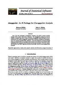
2.4. Variance estimates In order to estimate the diffusion tensor using (11) and (12) we need to model the heteroscedastic variances σ~2 . Empirical evidence from various DWI data sets with replicated b,i non-diffusion weighted images suggests the existence of a wide range of image intensity values where the standard deviation σ~b,i can be well approximated by a linear function of the observed image intensity. Figure 1 illustrates the situation for two data sets with replicated S0 images. The linear dependence between noise variance and image intensity seems to reflect properties of physiological noise. We therefore use the following model for the error standard deviations  θ~b,i < A0   σ 0 + σ 1 A0 σ0 + σ1 θb,i A0 ≤ θ~b,i < A1 σ~b,i =   σ +σ A A1 ≤ θ~b,i 0 1 1

(13)

Here A0 is set to the minimum, over voxel within the head, intensity in non-diffusion weighted images. For A1 we use the 0.99 quantile of S0 intensities within the head. The choice of A0 and

7

Journal of Statistical Software

(B) Variance modeling: data set 2

0

0

Error standard deviation Grey value density 10 20

Error standard deviation Grey value density 50 100 150

30

200

(A) Variance modeling: data set 1

1000

1500

2000

2500 3000 Grey value

3500

4000

4500

100

200

300 Grey value

400

500

Figure 1: Local polynomial estimates of mean standard deviation as a function of mean grey value (solid) and density of mean grey values (dotted) observed for two DWI data sets with replicated non-diffusion weighted images S0 . The red and blue curves correspond to variance estimates obtained from replicates (red) and mean variance estimates obtained from single images (blue), respectively, using the model (13) in both cases. Data set 1 is not registered causing a positive bias in voxelwise variance estimates from replications. The dashed curves in the left panel provide the corresponding estimates using mean absolute deviation (mad) as an alternative to voxelwise standard deviation (sd) to lower this effect. For a description of the two data sets see Section 5.5.

A1 coincides with the range where we observe approximative linearity between the standard deviation and the mean. The parameters σ0 and σ1 are estimated by linear regression between estimated voxelwise standard deviations and mean grey values in the case of a replicated non-diffusion weighted image or from a single non-diffusion weighted image using adaptive smoothing with explicit specification of the dependency between mean and standard deviation, see Polzehl and Tabelow (2007). In both cases the estimates will be restricted to use voxel with intensity within the range (A0 , A1 ).

3. Handling Rician bias in diffusion weighted images 3.1. Rician bias Thermal noise in DWI can be modeled as additive Gaussian noise in both the real and imaginary part of the signal in k-space. After fast Fourier transform into image space the resulting observed signal follows a Rician distribution (Rice 1945) with parameters ζ and σ. ζ is the signal of interest while σ corresponds to the standard deviation of the errors in k-space.

8

dti: Structural Adaptive Smoothing in Diffusion Tensor Imaging

The density of Rician distribution is given by p(x) =

x2 + ζ 2 xζ x exp(− )I0 ( 2 ), 2 2 σ 2σ σ

(14)

where I0 is the modified zeroth-order Bessel function of the first kind. Mean and variance of the Rician distribution are given by EX = σ

p π/2L1/2 (−ζ 2 /2σ 2 )

DX = 2σ 2 + ζ 2 −

πσ 2 2

(15)

L21/2 (−ζ 2 /2σ 2 )

(16)

with L1/2 (x) = ex/2 [(1 − x)I0 (−x/2) − xI1 (−x/2)].

(17)

For large ζ/σ we get EX ≈ ζ, while for small ζ/σ the expected value of the observed signal is significantly larger than the parameter of interest ζ. This effect is called Rician bias and is more pronounced in the diffusion weighted images where the signal is attenuated, see Equation 1. The Rician bias in the diffusion weighted images may lead to a bias in the estimated tensors as well as in quantities derived from the tensor, see Basu, Fletcher, and Whitaker (2006). We therefore include a correction for Rician bias in our implementation.

3.2. Correction for Rician bias In order to avoid the Rician bias we need to estimate the parameters ζ and σ of the underlying Rician distribution from the measured signals S. Let us assume we have samples Ngrad Sn = {S1,k , . . . , Sn,k }k=1 drawn from a Rician distribution Rice(ζk , σ). This resembles the situation within DWI data assuming that the noise variance in k-space does not depend on the gradient direction. For identifiability of the distribution parameters we need n > 1, which can be achieved by locating voxel with similar parameters within a local vicinity, see Section 4. Let now W = {w1 , . . . , wn } define a set of weights. We can then define a weighted log-likelihood function as l(Sn ; ζ, σ, W ) =

Ngrad n X X

wj

k=1 j=1

2 + ζ2 Sj,k Sj,k k log 2 − + log I0 2 σ 2σ



Sj,k ζk σ2

! .

(18)

Differentiating with respect to the parameters ζ and σ 2 yields conditions for the likelihood estimate of ζ = (ζ1 , . . . , ζNgrad ) and σ 2 d l(Sn ; ζ, σ, W ) = dζk d l(Sn ; ζ, σ, W ) = dσ 2

n X j=1

I1



I0



wj

Ngrad n X X k=1 j=1

Sj,k ζk σ2 Sj,k ζk σ2



  Sj,k − ζk

1 wj − 2 + σ

n X

wj = 0

(19)

j=1 2 Sj,k

+

2σ 4

ζk2



Sj,k ζk σ2



 Sj,k ζk  − S ζ  = 0. k σ4 I0 j,k 2 σ I1

9

Journal of Statistical Software The estimates ζˆk and σˆ2 can thus be obtained as fixpoints of   Sj,k ζˆk n I X 1 ˆ2 1 ζˆk = Pn wj  σ ˆ  Sj,k S ζ j=1 wj j=1 I0 j,kˆ2 k σ     Sj,k ζˆk Ngrad n 2 2 I1 X X  Sj,k + ζˆk ˆ2 1  Pn σˆ2 = wj  −  σ ˆ  Sj,k ζˆk  Sj,k ζk Ngrad j=1 wj 2 I0 k=1 j=1 ˆ2

(20)

σ

through iteration. As initial estimate we use the corresponding likelihood estimates for a Gaussian distribution (0) ζˆk =

(0) σˆ2 =

n X

1 Pn

j=1 wj j=1

Pn

2 j=1 wj ) P Pn ( j=1 wj )2 − nj=1 wj2

(

(21)

wj Sj,k

Ngrad

1 Pn

j=1 wj

Ngrad n X X

wj (Sj,k − ζˆk )2 .

k=1 j=1

(0) (0) We use a prespecified number of iteration steps depending on the ratio ζˆk /ˆ σk , i.e., no iteration if the ratio is larger than 10 and up to 6 iterations if the ratio is small.

If an estimate of σ can be obtained from the background it can be used in (20) alternatively, see e.g., Fillard et al. (2007a).

4. Structural adaptive smoothing We recently proposed a new structural adaptive smoothing algorithm for diffusion weighted data in the context of the diffusion tensor model (Tabelow et al. 2008). The approach reduces the error of the estimated tensor directions and tensor characteristics like fractional anisotropy by smoothing the observed DWI data. The application of a standard Gaussian filter would be highly inefficient in the DTI applications in view of the anisotropic nature of the diffusion tensor and sharp boundaries between region with different tensor characteristics. Indeed, the tensor direction remains constant mainly along the fiber directions. Averaging over a large symmetric neighborhood of every voxel would thus lead to a loss of directional information. In order to avoid such a loss our smoothing procedure sequentially determines at increasing scales local weighting schemes with positive weights for voxel that show similar characteristics. To achieve this we employ the structural assumption that for every voxel there exists a vicinity in which the diffusion tensor is nearly constant. This assumption reflects the fact that the structures of interest are regions with a homogeneous fractional anisotropy, a homogeneous diffusivity, and a locally constant direction field. The shape of this neighborhood can be quite different for different voxel and cannot be described by few simple characteristics like bandwidth or principal directions. The algorithm for the case of linear tensor estimates using model (9) has been described in detail in Tabelow et al. (2008). Here, we shortly present a modified algorithm that is based on the nonlinear regression model (10) for the diffusion tensor and incorporates the Rician bias correction developed in the previous section:

10

dti: Structural Adaptive Smoothing in Diffusion Tensor Imaging

Algorithm: ˆ Initialization: Set k = 1, initialize the bandwidth h(1) = ch . For each voxel i initialize (0) ˆ (0) and θˆ(0) by Equation 12, set N (0) = 1. Estimate the ζˆ~ = S~b,i with the data, and D i 0,i i b,i

parameters σ0 and σ1 of the variance model (13). ˆ Adaptation: For each voxel pair i, j, we compute the penalty (k−1)

(k)

sij

=

h    i Ni ˆ(k−1) , θˆ(k−1) , D ˆ (k−1) − R ζˆ(k−1) , θˆ(k−1) , D ˆ (k−1) R ζ ·,i 0,j j ·,i 0,i i λCi (g, h(k−1) )

(k−1) (k) with the risk R based on the previous estimates ζˆ·,i at voxel i. sij measures the (k−1) ˆ (k−1) at voxel i and j. Weights statistical difference between the estimates θˆ and D 0

are computed as

    (k) ˜ (k−1) )/h(k) Kst s(k) , wij = Kloc ∆(i, j, D i ij with appropriate kernel functions Kloc and Kst , an anisotropic distance function ∆, and ˜ (k−1) , see Tabelow et al. (2008) for details. a regularized tensor estimate D i ˆ Rice bias correction and estimation of diffusion weighted images: Compute (k) (k) (k) ζˆ.,i = (ζˆ1,i , . . . ζˆNgrad ,i ) by maximizing the log-likelihood (18) (k) (k) ζˆ.,i = argζ max l(Sn ; ζ, σ, Wi ) ζ,σ

(k)

using the weighting scheme Wi

(k)

(k)

= (wi1 , . . . , win ) and evaluating Equations 21,20.

ˆ Parameter estimation: Compute new estimates of the expected non-diffusion weighted images θ0,i and diffusion tensors Di as

(k)

see (12). Set Ni

=



(k) θˆ0,i



ˆ (k) D i

  = arg min R(ζˆ(k) , θ, D), θ,D

.,i

(k) j=1 wij .

Pn

ˆ Stopping: Stop if k = k ∗ for a preselected number of iteration steps, otherwise set h(k+1) = ch h(k) , increase k by 1 and continue with the adaptation step.

The term Ci (g, h(k−1) ) provides an adjustment under the assumption that spatial smoothness of the errors can be modeled by a convolution of independent errors with a Gaussian kernel of bandwidth g, see e.g., Tabelow et al. (2008) or Tabelow, Polzehl, Voss, and Spokoiny (2006) (k) for details. The Rician bias correction can be omitted using S.,i instead of ζˆ.,i in all steps. λ is the main parameter of the procedure and can be determined by simulations, see Polzehl and Spokoiny (2006) or Tabelow et al. (2008) for details.

Journal of Statistical Software

11

5. Using the package dti This document refers to the versions 0.6-0 or later of the dti package which is available from the Comprehensive R Archive Network (CRAN) at http://CRAN.R-project.org/package=dti. The software is under constant development, see Section 5.8 for details on the plans for the next future. Changes are documented in the HISTORY file of the package. For the analysis of diffusion weighted data, there is an overlap in functionality needed from other packages. In order to fully use the package dti it is therefore required to install the packages fmri (Tabelow and Polzehl 2009c) for reading and writing medical imaging formats like ANALYZE, NIfTI, or DICOM as well as adimpro (Tabelow and Polzehl 2009a) and rgl (Adler and Murdoch 2009) for visualization. These packages can also be downloaded from CRAN. For a typical analysis we assume the DWI data to reside in a directory, say "datadir", and the gradient matrix in a file, say "gradient.txt". A script for the analysis could then have the form R> R> R> R> R> R> R>

library("dti") grad