The R System – An Introduction and Overview
J H Maindonald Centre for Mathematics and Its Applications Australian National University.
© J. H. Maindonald 2005, 2006. Permission is given to make copies for personal study and class use.
Languages shape the way we think, and determine what we can think about. [Benjamin Whorf.] S has forever altered the way people analyze, visualize, and manipulate data... S is an elegant, widely accepted, and enduring software system, with conceptual integrity, thanks to the insight, taste, and effort of John Chambers. [From the citation for the 1998 Association for Computing Machinery Software award.]
2
John H. Maindonald, Centre for Mathematics & Its Applications, Mathematical Sciences Institute, Australian National University, Canberra ACT 0200, Australia,
[email protected] http://www.maths.anu.edu.au/~johnm July 18, 2007
This document aims to cover the basics of use of R as briefly as possible. There will be occasional references to DAAGUR: Maindonald, J. H. & Braun, J. B. 2007. Data Analysis & Graphics Using R. An ExampleBased Approach. Cambridge University Press, Cambridge, UK, 2007. http://www.maths.anu.edu.au/~johnm/r-book.html
5
plot(1:6, rep(4.5, 6), cex=1:6, col=1:6, pch=0:5, xlim=c(1, 6.5), ylim=c(0,5.4), xlab="", ylab="")
4
●
abc The result is 4. The [1] says, a little strangely, “first requested element will follow”. Here, there is just one element. The > indicates that R is ready for another command. The exit or quit command is > q () Depending on the platform, alternatives may be to click on the File menu and then on Exit, or to click on the X in the top right hand corner of the R window. There will be a message asking whether to save the workspace image. Clicking Yes (the safe option) will save the objects that remain in the workspace – any that were there at the start of the session and any that have been added since. Commands may continue over more than one line. By default, the continuation prompt is + As with the > prompt, this is generated by R. Any attempt to include it in the code that is entered will generate an error! 11
12
CHAPTER 2. AN OVERVIEW OF R
For the names of R objects or commands, case is significant. Thus Myr (millions of years) is different from myr. (Myr is a column in the data frame molclock, used in Exercises 1 and 2 in Section 4.10). For file names on Windows systems, the Microsoft Windows conventions apply, and case does not distinguish file names. On Unix systems (the Mac OS X version of Unix is an exception) case in file names is significant. Further points are: o The quit command (“quit from the R session”) is the function call q(). Typing q on its own, without the parentheses, displays the text of the function on the screen. o Multiple commands may appear on a line, with the semicolon (;) as the separator. o The # symbol indicates that what follows, on that line, is comment.
Practice with R commands Try the following 1:5 mean (1:5) sum (1:5)
# The numbers 1 , 2 , 3 , 4 , 5
# Apply the sum function to the # the vector of numbers 1 , 2 , 3 , 4 , 5 (2:5)^10 # 2 to the power of 10 , 3 to the power of 10 , ... log2 ( c (0.5 , 1 , 2 , 4 , 8)) # Values that differ by a factor of 2 # are , on this scale , one unit apart .
The R language has the abilities for evaluating arithmetic and logical expressions that are available in most languages. It uses functions to extend these basic arithmetic and logical abilities.
2.2
Demonstrations
There are a number of demonstrations that give useful indications of R’s abilities, especially for graphics. To get a list of available demonstration, type: demo () Visually interesting demonstrations are: demo ( image ) demo ( graphics ) demo ( persp ) demo ( plotmath ) library ( lattice ) demo ( lattice )
# Mathematical symbols can be visually interesting # Demonstrates lattice graphics
Especially for demo(lattice), it pays to stretch the graphics window to cover a substantial part of the screen. Place the cursor on the lower right corner of the graphics window, hold down the left mouse button, and pull. Try also demo ( package = . packages ( all . available = TRUE )) Also interesting is: library ( vcd ) demo ( mosaic )
# The vcd package must of course be installed .
2.3. A SHORT R SESSION
13
Examples that are included on help pages Additionally, note that most R functions have examples on their help pages. To run all the examples that are provided for plot(), type: example ( plot ) You’ll need to press the Enter key to show the first plot and to move from one plot to the next.
2.3
A Short R Session
We will work with the data set shown in Table 2.1: Aird’s Guide to Sydney Moon’s Australia handbook Explore Australia Road Atlas Australian Motoring Guide Penguin Touring Atlas Canberra - The Guide
Volume (mm3 ) 351.00 955.00 662.00 1203.00 557.00 460.00
Weight (g) 250.00 840.00 550.00 1360.00 640.00 420.00
type Guide Guide Roadmaps Roadmaps Roadmaps Guide
Table 2.1: Weights and volumes, for six Australian travel books.
Entry of vector elements from the command line Data may be entered from the command line, thus: volume volume [6] [1] 460 > # # Ratio of weight to volume , i . e . , density > round ( weight / volume ,2) [1] 0.71 0.88 0.83 1.13 1.15 0.91
Notice the use of # to preface the comment, causing it to be ignored by the command line interpreter.
A simple plot
800
●
●
● ●
400 600 800
Figure 2.1: Weight versus volume, for six Australian travel books. # # Code plot ( weight ~ volume , pch =16 , cex =1.5) # pch =16: use solid blob as plot symbol # cex =1.5: point size is 1.5 times default # # Alternative plot ( volume , weight , pch =16 , cex =1.5)
●
400
weight
1200
●
1200
volume
Figure 2.1 plots weight against volume, for the six Australian travel books. The argument weight ~ volume is a graphics formula. The “formulae” that are used in specifying models, and in the functions xtabs() and unstack(), take a similar form. The axes can be labeled: plot ( weight ~ volume , pch =16 , cex =1.5 , xlab = " Volume ( cubic mm ) " , ylab = " Weight ( g ) " )
Labeling of the points (e.g., with the species names) can be done interactively, with the identify() command. Type: identify ( weight ~ volume , labels = description )
Then click the left mouse button above or below a point, or on the left or right, depending on where you wish the label to appear. Repeat for as many points as you want labelled. Depending on the computer system, either click outside the graphics area to terminate the labelling, or click the right mouse button outside the figure area. Alternatively, use text() to place labels on all the points. There are extensive abilities that may be used to control the formatting and layout of plots, and to add features such as special symbols, fitted lines and curves, annotation (including mathematical annotation), colors and so on. A later chapter (Chapter 5) is devoted to graphics.
2.4. DATA FRAMES – GROUPING TOGETHER COLUMNS OF DATA
2.4
15
Data frames – Grouping together columns of data
Data Frames Data frames
Data frames are the preferred way to make data available to modeling functions.
Creating data frames
1: Enter from the command line, 2: Use read.table() to input from a file.
Columns of data frames
travelbooks$weight or travelbooks[, "weight"] or travelbooks[, 4] Use the data parameter, if available, in a function call Use attach(), e.g., attach(travelbooks) Use with(), e.g. with(travelbooks, plot(weight volume))
The following demonstrates the use of a data frame to group together, under the name travelbooks, the several columns of Table 1. # # NB , the row names will now be shortened travelbooks ls () [1] " volume " " weight " > ls ( pattern = " ^ w " ) 19
20
CHAPTER 3. THE WORKING ENVIRONMENT OF AN R SESSION
[1] " weight " Cautious users will from time to time save (back up) the current workspace image. The command save.image()) saves everything in the workspace, by default into a file named .RData in the working directory. Or, depending on the implementation, clicking on the relevant menu item will save an image of the workspace. Before saving the workspace, consider use of rm() to remove objects that are no longer required. Saving the workspace image will then save everything that remains. Upon quitting from R (type q(), or use the relevant menu item), users are asked whether they wish to save the current workspace. The workspace is reloaded next time an R session is started in the directory. The workspace is at the base of a search list that gives access to packages, objects in other directories, etc.
Setting the Working Directory When working from a Unix or Linux command line, the working directory is the directory in which the session is started. When an session is started by clicking on a Windows icon, the icon’s Properties specify the Start In directory. The default choice, usually an R installation directory, is not satisfactory for long-term use, and should be changed. It is good practice to use a separate working directory for each different project. On Windows systems, copy an existing R icon, rename it as desired, and change the Start In directory to the new working directory. It is also possible to change the working directory once a session has started. This can be done either from the menu (if available) or from the command line. Before making such a change, be sure to save the existing workspace, if it is to be kept. Then, once the working directory has been changed, load the new workspace.
3.2
Saving and retrieving R objects
Image files, created using save() or save.image(), may contain arbitrary R objects. One or more objects can be saved to an image file at any time during a session. Upon quitting a session, the user is offered the option of saving the workspace in the default image file. The following demonstrate the explicit use of the save() and load() commands: save ( volume , weight , file = " books . RData " ) # Can save many objects in the same file load ( " books . RData " ) # Recover the saved objects The function save.image() is a variation on save() that saves the contents of the workspace, by default in the file .RData. The contents of any .RData file in the working directory are automatically loaded when a new session is started. An alternative to saving the objects in an image file is to save them, in a text format, as dump files:the above use of save() is: dump ( c ( " volume " , " weight " ) , file = " books . R " ) The objects can be recreated from this “dump” file by inputting the lines of books.R one by one at the command line. The following command restores both objects to the workspace: source ( " books . R " ) For day to day use, image .RData files are in general preferable to dump files. The same checks are performed on dump files as if the text had been entered at the command line. These may be unwanted, and they slow down entry of the data or other object. For archival storage, dump (.R) files may be preferable. For added security, retain a printed version. If a problem arises (from a system change, or because the file has been corrupted), it is then possible to check through the file line by line to find what is wrong.
3.3. INSTALLATIONS, PACKAGES AND SESSIONS
21
Writing data frames to text files Use the function write.table() to write a data frame to a text file. More generally, to save several objects (data frames or any other R object) in the one file, use dump() (to save in a text format) or save.image(), as noted above.
3.3
Installations, packages and sessions
Packages & the Search List Packages
Packages are collections of R functions and/or data. (Binary R distributions include recommended packages. Install other packages, as required, prior to their use.)
library()
Use library() to attach a package, e.g., library(DAAG) Once attached, a package is added to the search list, i.e., to the list of “databases” that R searches for functions and/or data.
attach()
Use attach() to attach data frames or image (.RData) files. The data frame or image file is added to the search list, usually in position 2, i.e., following the workspace (.Globalenv)
3.3.1
The architecture of an R installation – Packages
An R installation is structured as a library of packages. • All installations should have the base packages (one of them is called base) , which provide the superstructure for other packages. • Binaries that are available from CRAN sites include, also, all the recommended packages. • Other packages can be installed as required. A number of packages are by default attached at the start of a session. Other packages can be attached (use library()) as required. To discover which packages have been attached, enter: sessionInfo () Installation of R packages Installation from the R menu on a Windows or MacOS X system calls the function install.packages(). Alternatively, this function can be invoked directly. See help(install.packages) The menu can also be used to install packages from local zip or (under MacOS X) .tar.gz files. Note also download.packages() (this takes a list of package names and a destination directory, downloads the newest versions of the package sources and saves them in ‘destdir’) and update.packages() (outdated packages are reported and for each outdated package the user can specify if it should be automatically updated). On Unix and Linux systems, the relevant gzipped tar files, once downloaded to a storage device, can be installed using the shell command: R CMD INSTALL For installation of packages that are in a local directory from the command line, call install.packages() with pkgs giving the files (with path, if necessary), and with the argument repos=NULL. If for example the binary DAAG 0.91.zip has been downloaded to D:\tmp\, it can be installed thus install . packages ( pkgs = " D : / DAAG _ 0.91. zip " , repos = NULL ) In the R command line, be sure to replace the usual Windows backslashes by forward slashes.
22
CHAPTER 3. THE WORKING ENVIRONMENT OF AN R SESSION
3.3.2
The search path: library() and attach()
The search path is important for determining where R looks for R objects (functions or data) that are required in an R session, and that cannot be found in the workspace. At any time in a session, the R system has a search path (or list) that determines where it looks for objects. To get a snapshot of the search list, type: > search () [1] " . GlobalEnv " [5] " package : methods " [9] " Autoloads "
" package : xtable " " package : stats " " package : base "
" package : MASS " " package : vcd " " package : graphics " " package : utils "
Technically, these are called “databases”. The search path is used to structure the search for R objects. The database ”.GlobalEnv” is the user’s workspace, which is at the base of the search path. The attach() and library() commands extend the search list. Attachment of R packages The use of library() to attach an R package extends the search list. The system then looks in the package database for objects that are not in the user workspace. If at some point (often the end of the session) the workspace is saved, and objects that were added have not been explicitly removed, they will be saved as part of the workspace. If saved in the default .RData image file in the working directory, the workspace will be automatically loaded when a new session is next started in that working directory. Use the function .path.package() to get the path of a currently attached package. By default, this information is given for all loaded packages. Attachment of image files As noted earlier, the function attach() extends the search list, by simplifying access to the columns of data frames or to the elements of lists, or by giving access to an image file that is stored somewhere. Additionally, any R image file can be attached, either from the current working directory, or from any other directory. For example: attach ( " books . RData " ) The workspace then has access to objects in the file books.RData. The file becomes a further “database” on the search list, separate from the workspace. If however the object is modified, the modified copy does become part of the workspace. In order to detach such a database, proceed thus: detach ( " file : books . RData " )
3.4
Summary Each R session has a working directory. This is the directory where R will by default look for files or store files that are external to R. User-created objects appear appear in the workspace. At the end of a session (and perhaps from time to time during the session), an image of the workspace will typically be saved into the working directory. It is usually best to keep a separate workspace and associated working directory, for each major project.
Chapter 4
Objects and Functions Different types of data objects: Vectors
These collect together elements that are all of one mode. (Possible modes are “logical”, “integer”, “numeric”, “complex”, “character”) and “raw”)
Factors
These identify categories (levels) in categorical data. They make it easy to write down model formulae that account for categorical effects (Factors are very like vectors, but do not quite manage to be vectors! Why?)
Data frame
A list of columns – same length; modes may differ.
Lists
Lists group together an arbitrary collection of objects (These are recursive structures; elements of lists are lists.)
NAs The handling of NAs (missing values) can be tricky. The R system does not keep a rigid separation between data objects and functions. For, example, data that will be analyzed may be stored along with functions in the same object, usually a list. We start this chapter by noting data objects that may appear as columns of a data frame.
4.1
Columns of Data, & Data Frames
Columns of a data frame must be vectors or factors. Factors will be discussed later. For now, note that they do not quite meet the requirement to be a vector.
4.1.1
Vectors
Examples of vectors are c (2 ,3 ,5 ,2 ,7 ,1) 3:10 # The numbers 3 , 4 ,.. , 10 c ( TRUE , FALSE , FALSE , FALSE , TRUE , TRUE , FALSE ) c ( " cherry " ," mango " ," apple " ," prune " ) As noted in Chapter 1, vectors may have mode logical, numeric or character. The first two vectors above are numeric, the third is logical (i.e. a vector with elements of mode logical), and the fourth is a string vector (i.e. a vector with elements of mode character). The c in c(2, 3, 5, 7, 1) has the meaning is: “Join (concatenate) these numbers together into a vector”. Existing vectors may supply some or all of the elements that are to be concatenated. The missing value symbol, which is NA, can be included as an element of a vector. 23
24
CHAPTER 4. OBJECTS AND FUNCTIONS
Subsets of Vectors There are four common ways to extract subsets of vectors. 1. Specify the subscripts of the elements that are to be extracted, e.g. > x x [ c (2 ,4)] # Extract elements ( rows ) 2 and 4 [1] 11 15 Negative numbers may be used to omit elements: > x x [ - c (2 ,3)] [1] 3 15 12 2. Specify a vector of logical values. The elements that are extracted are those for which the logical value is TRUE. Thus suppose we want to extract values of x that are greater than 10. > x >10 # This generates a vector of logical ( TRUE or FALSE ) [1] F T F T T > x [ x > 10] [1] 11 15 12 Arithmetic relations that may be used in the extraction of subsets >=, ==, and !=. The first four compare magnitudes, == tests for equality, and != tests for inequality. 3. For vectors of named elements, the elements may be identified by name: > library ( DAAG ) > cuckooEgglengths cuckooEgglengths [1] 22.3 23.1 22.5 22.6 23.1 21.1 22.6 > > # # Assign names to the vector elements > names ( cuckooEgglengths ) cuckooEgglengths meadow pipit hedge sparrow robin wagtails 22.3 23.1 22.5 22.6 tree pipit wren yellow ammer 23.1 21.1 22.6 > > # # Names can be used to extract elements > cuckooEgglengths [ c ( " hedge . sparrow " , " robin " , " wren " )] hedge sparrow robin wren 23.1 22.5 21.1 4. Use subset(), with the vector as the first argument, and a logical statement that identifies the elements to be extracted as the second argument. For example: > subset ( cuckooEggLengths , cuckooEggLengths > 23) [1] 23.10 23.10 23.05
4.1.2
Factors
Factors are column objects whose elements are integer values 1, 2, . . . , k, where k is the number of levels. They are distinguished from integer vectors by having the class factor and a levels attribute. They provide, in data frames, the default way to store text string information.
4.1. COLUMNS OF DATA, & DATA FRAMES
25
The character vector c("cherry","mango","apple","prune","cherry","prune") might equally well be stored as a factor, thus: > fruit fruitfac as ( fruitfac , " numeric " ) [1] 2 3 1 4 2 4 > levels ( fruitfac ) [1] " apple " " cherry " " mango " " prune " Notice that, by default, the levels are taken in alphanumeric order. Internally, the factor is stored as the integer vector 2, 3, 1, 4, 2, 4. It has stored with it the table: 1 "apple"
2 "cherry"
3 "mango"
4 "prune"
Thus, the numeric values are codes for text strings, with information that matches the codes to a unique set of text strings stored in the separate table. The order can be specified. For example: > # # Take fruit in order of stated glycemic index (15 , 22 , 38 , 55) > fruitfac levels ( fruitfac ) [1] " prune " " cherry " " apple " " mango " Changing the levels in this way can be useful where factor levels are used, as in some lattice graphs that have one panel for each factor level, to determine the order in which plots appear. Note that the function factor(), with the levels argument specified, can be used both to specify the order of levels when the factor is created, or to make a later change to the order. Incorrect spelling of the level names generates missing values, for the level that was mis-spelled. Try: fruitfac fruitfac fruitfac == " cherry " [1] TRUE FALSE FALSE FALSE TRUE Section 7.2 has detailed examples of the use of factors in model formulae and the resultant model matrices.
Ordered factors In addition to factors, note the existence of ordered factors, created using the function ordered(). For ordered factors, the order of levels implies a relational ordering. For example: > windowTint windowTint [1] lo med hi lo med hi Levels : lo < med < hi
26
CHAPTER 4. OBJECTS AND FUNCTIONS
4.1.3
Subsets of data frames
To extract the first three rows of the data frame travelbooks, specify travelbooks[1:3,]. For columns 1 to 3, specify travelbooks[, 1:3]. Negative indices can be used to omit rows and/or columns. However positive and negative indices cannot be mixed in the same vector of subscripts. Additionally, a vector of logicals (TRUEs and FALSEs) may be used to extract rows and/or columns. First observe that travelbooks$weight > 500 is a vector of logicals: > travelbooks $ weight > 500 # # Result is a vector of logicals [1] FALSE TRUE TRUE TRUE TRUE FALSE Thus, travelbooks[travelbooks$weight > 500, ] can be used to extract rows for which weight is greater than 500. A more elegant approach is to use the function subset(): > subset ( travelbooks , weight > 500) thickness width height weight volume type Moon ' s Australia handbook 3.9 13.1 18.7 840 955 Guide Explore Australia Road Atlas 1.2 20.0 27.6 550 662 Roadmaps Australian Motoring Guide 2.0 21.1 28.5 1360 1203 Roadmaps Penguin Touring Atlas 0.6 25.8 36.0 640 557 Roadmaps
4.1.4
Data frames – Lists of Columns
Data frames are lists of columns. Columns can be vectors or vector-like objects.1 One consequence is that use of the subscript notation to extract a row from a data frame gives a different data structure from use of the subscript notation to extract a column. Specifically: travelbooks$volume (or travelbooks[,"volume"] or travelbooks[,1]) is a vector. The result of travelbooks["Canberra - The Guide", ] or travelbooks[6, ] is a data frame, i.e., a special form of list. The syntax unlist(travelbooks[6, ]) can be used to turn such a list into a vector. Be careful to distinguish data frames from matrices. Data frames in which all elements have the same mode (commonly, all numeric) are in certain restricted contexts exchangeable with matrices, but that is not true in general. Matrices, although laid out in a rectangular format, have a vector structure, where successive columns follow one after another. Matrices will be discussed further in Section 4.4.
4.1.5
Inclusion of character vectors in data frames
When data frames are created, whether by use of read.table() from a file, or by an assignment on the command line in which columns of data become columns in the data frame, character vectors are converted into factors. Thus, the final column (type) of travelbooks became, by default, a factor. To prevent such type conversions, specify as.is=TRUE. Section 10.1 has furtehr information on the input of data, using read.table(), from a file.
4.2
Missing Values, Infinite Values and NaNs
Problems with missing values, infinite values and NaNs are a common reason why functions fail. An understanding of the conventions for arithmetic with NAs will reduce the scope for unwelcome surprises. Any arithmetic or logical operation with NA generates an NA. The consequences are more farreaching than might be immediately obvious. Use is.na() to test for a missing value: v > is . na ( c (1 , NA , 3 , 0 , NA )) [1] FALSE TRUE FALSE FALSE TRUE 1 Factors,
which will be discussed later, are the vector-like objects that are in mind.
4.3. THE USE OF DATA FRAMES IN CORRELATION AND REGRESSION
27
An expression such as c(1, NA, 3, 0, NA) returns a vector of NAs, and cannot be used to test for missing values. > c (1 , NA , 3 , 0 , NA ) == NA [1] NA NA NA NA NA As the value is unknown, it might or might not be equal to 1, or to another NA, or to 3, or to 0. Note that the attempt to assign values to an expression whose subscripts include missing values generates an error. > y y [ y > 0] [1] 1 NA 3 NA > y [ y > 0] test . df test . df x y 1 1 1 2 2 2 3 NA 3 > complete . cases ( test . df ) [1] TRUE TRUE FALSE > na . omit ( test . df ) x y 1 1 1 2 2 2
4.3
The Use of Data Frames in Correlation and Regression
The purpose here is to indicate how R uses data frames in statistical calculations, using the data in the data frame travelbooks. We will first add, to the data frame travelbooks, new columns area (area of page), and density (weight to volume ratio): > travelbooks $ area travelbooks $ density names ( travelbooks ) # Check full set of column names [1] " thickness " " width " " height " " weight " " volume " [7] " area " " density "
" type "
2 Note however that sqrt(-1+0i) returns sqrt(0+1i). R distinguishes between -1, which is a real number, and -1+0i which is a complex number.
28
CHAPTER 4. OBJECTS AND FUNCTIONS
A first step is to call the generic function plot with travelbooks as argument: pairs ( travelbooks [ , -6]) # # Alternative plot ( travelbooks [ , -6])
# Omit column 6
Not unexpectedly, there are relationships between width and height, and between weight and volume. Less expected, perhaps, is the indication of a relationship between density and area.
Correlation calculations The function cor(), with a matrix or data frame as argument, calculates the correlation matrix for the columns. By default, it gives the Pearson product-moment linear correlation. For example: > round ( cor ( travelbooks [ , -6]) ,2) thickness width height weight volume area density thickness 1.00 -0.47 -0.77 0.40 0.58 -0.59 -0.16 width -0.47 1.00 0.91 0.44 0.28 0.98 0.80 height -0.77 0.91 1.00 0.13 -0.08 0.97 0.67 weight 0.40 0.44 0.13 1.00 0.97 0.30 0.69 volume 0.58 0.28 -0.08 0.97 1.00 0.12 0.51 area -0.59 0.98 0.97 0.30 0.12 1.00 0.77 density -0.16 0.80 0.67 0.69 0.51 0.77 1.00
Dependence of weight on volume One way to investigate is to examine the regression relationship: > wtvol . lm wtvol . lm Call : lm ( formula = weight ~ volume , data = travelbooks ) Coefficients : ( Intercept ) -137.768
volume 1.167
Notice that we saved the regression (lm) object, with the name wtvol.lm. This can be printed or summarized or used to extract other information, or be used as the basis for various graphs. The large intercept is perhaps unexpected. We might expect weight to be proportional to volume. To force the line through the origin, do the following: wtvol0 . lm travelmat dim ( travelmat ) # Equivalent to attr ( travelmat , " dim ") [1] 6 4 > attr ( travelmat , " dim " ) [1] 6 4
Removal of the dimension attribute The dimension attribute can be changed or removed, thus: > travelvec dim ( travelvec ) travelvec [1] 1.3 3.9 1.2 2.0 0.6 1.5 11.3 13.1 20.0 21.1 [11] 25.8 13.1 23.9 18.7 27.6 28.5 36.0 23.4 250.0 [21] 550.0 1360.0 640.0 420.0 > # Use of as ( travelmat , " vector ") is however preferable > # For these data , why would one do this ?
840.0
Submatrices To extract the first three rows of the matrix travelmat, specify travelmat[1:3,]. For columns 1 to 3, specify travelmat[, 1:3]. Negative indices can be used, as for data frames to omit rows and/or columns.3 3 Note
that the $ notation is designed for use with data frames and other list objects, and is not relevant to matrices.
30
CHAPTER 4. OBJECTS AND FUNCTIONS
4.4.1
Matrix Manipulations
Let X, Y and B be numeric matrices. Some of the possibilities are: X + Y X * Y X %*% B solve (X , Y ) svd ( X ) qr ( X )
# # # # # #
Elementwise addition ( The dimensions must agree ) Elementwise multiplication ( The dimensions must agree ) Matrix multiplication ( X is n by k ; B k by m ) Solve X B = Y ( X is n by k , Y n by m , B k by m ) Singular value decomposition of X QR decomposition of X .
Use matrices for efficient computation For working with large numerical arrays, the matrix structure can allow much faster computations than are possible with data frames. See Section 10.4
4.4.2
Data frames versus matrices
Data frames that consist entirely of numeric data are in some (but not all) contexts interchangeable with numeric matrices. There are however important differences. In some applications, e.g., the analysis of microarray data, both of these types of object are in wide use. Note that for a matrix length() returns the number of elements, while for a matrix it retuens the number of columns: > length ( travelbooks ) # travelbooks is a list of 7 vectors [1] 5 > length ( as ( travelbooks [ ,1:4] , " matrix " )) # matrix has 28 elements [1] 28 Functions are available to convert data frames into matrices, and vice versa. For example: travelmat wtvol . lm $ call lm ( formula = weight ~ volume , data = travelbooks )
Where an extractor function is available, use this in preference to accessing the specific list elements. Thus use: > coef ( wtvol . lm ) ( Intercept ) volume -137.767923 1.166812 > resid ( wtvol . lm ) Aird ' s Guide to Sydney -21.78300 Explore Australia Road Atlas -84.66144 Penguin Touring Atlas 127.85379
Moon ' s Australia handbook -136.53728 Australian Motoring Guide 94.09341 Canberra - The Guide 21.03453
Notice that the residuals carry the row names. We might prefer shorter row names. The various R modeling functions all return their own particular type of model object, always stored as a list. Note also that data frames are a specialized form of list, with the restriction that all columns must be vectors that all have the same length.
32
4.6
CHAPTER 4. OBJECTS AND FUNCTIONS
Functions
Different Kinds of Functions Generic They examine the object given as argument, before functions deciding what action is needed. Examples include print(), plot() & summary() Modeling functions
Use to fit statistical models. Thus note lm() for linear modeling. Output may be stored in a model object.
Extractor functions
Use extractor functions to obtain specific types of information (summary, coefficients, residuals, etc.) from model objects. Examples are summary(), residuals(), etc
User
Create functions that automate & document computations
Anonymous
Functions that are defined in place do not need a name
4.6.1
Built-In Functions
Common useful functions, for use with vectors Common Useful Functions are print() cat() length() mean() median() range() unique() diff() sort() order() cumsum() cumprod() rev() any() as() is()
is.na() str() args() numeric()
character()
# Prints a single R object # Prints multiple objects, one after the other # Number of elements in a vector or of a list
# # # # #
Gives the vector of distinct values Vector of first differences N. B. diff(x) has one less element than x Sort elements into order, but omitting NAs x[order(x)] orders elements of x, with NAs last
# # # # # # # # # # # # # #
reverse the order of vector elements Returns TRUE if there are any missing values Coerce argument 1 to class given by argument 2 e.g. as(1:6, "factor") Is argument 1 of class given by argument 2? is(1:6, "factor") returns FALSE is(TRUE, "logical") returns TRUE Returns TRUE if the argument is an NA Information on an R object Information on arguments to a function numeric(5) creates a numeric vector of length 5, with all elements 0. numeric(0) (length 0) can be useful. Create character vector; c.f. also logical()
The functions mean(), median(), range(), and a number of other functions, take the argument na.rm=TRUE; i.e., remove NAs, then proceed with the calculation. For example > mean ( c (1 , NA , 3 , 0 , NA ) , na . rm = T ) [1] 1.3
4.6. FUNCTIONS
33
Note that the function as() cannot be used to coerce a matrix to a data frame; use as.data.frame(). The function as() has, at present, no method for coercing a matrix to a data frame.
4.6.2
User-defined functions
The R language is a functional language. The function mean() calculates means, The function sd() calculates standard deviations. Here is a function that calculates mean and standard deviation at the same time: mean . and . sd mean . and . sd () mean sd 0.1067355 1.1383779 We get a different set of random numbers, and hence a different mean and SD, each time that the function is run with its default argument.
4.6.3
Information on R Objects
Information on data objects The function str() gives basic information on the object that is given as argument. > str ( travelbooks ) ' data . frame ' : 6 obs . of 6 variables : $ thickness : num 1.3 3.9 1.2 2 0.6 1.5 $ width : num 11.3 13.1 20 21.1 25.8 13.1 $ height : num 23.9 18.7 27.6 28.5 36 23.4 $ weight : num 250 840 550 1360 640 420 $ volume : num 351 955 662 1203 557 ... 4 Data
are from Lewontin, R. 1974. The Genetic Basis of Evolutionary Change.
34
CHAPTER 4. OBJECTS AND FUNCTIONS
$ type
: Factor w / 2 levels " Guide " ," Roadmaps " : 1 1 2 2 2 1
Information on function arguments A useful function is args(). It lists function arguments, together with default values, if any.
4.6.4
Tables and Cross-Tabulation
Use the function table() to make a table of counts. Use xtabs() for cross-tabulation, i.e., to determine totals of numeric values for each table category.
table() The function table() makes a table of counts. Specify one vector of values (often a factor) for each table margin that is required. A simple example is: library ( DAAG ) > table ( possum $ Pop , possum $ sex ) f m Vic 24 22 other 19 39 Here is a use of table() to count the number of NAs in the column bp (blood pressure) from the data frame Pima.tr2 that is in the MASS package. > library ( MASS ) > table ( is . na ( Pima . tr2 $ bp )) FALSE 287
TRUE 13
By default, table() ignores NAs. Hence the need for a check of the following type, here using sapply() function. This can be used with a data frame as its first argument to apply the function specified as its second argument in parallel to all columns of the data frame, to give the number of NAs in each column of the data frame Pima.tr2 > sapply ( Pima . tr2 , function ( x ) sum ( is . na ( x ))) npreg glu bp skin bmi ped age type 0 0 13 98 3 0 0 0 The action needed to get NAs tabulated under a separate NA category depends, annoyingly, on whether or not the vector is a factor. If the vector is not a factor, specify exclude=NULL. If the vector is a factor then it is necessary to generate a new factor that includes NA as a level. Specify x catBP table ( catBP ) catBP (37.9 ,57] (57 ,76] (76 ,95] (95 ,114]
4.7. OPTION SETTINGS
22 170 > sum ( table ( catBP )) [1] 287
35
87
8
Notice that the 13 missing values, out of the total of 300, are not included in the table. This can be a trap. They are in catBP, as we can easily verify: > table ( is . na ( catBP )) FALSE 287
TRUE 13
Thus, above, we can do the following > catBP table ( catBP ) catBP (37.9 ,57] (57 ,76] (76 ,95] (95 ,114] 22 170 87 8 > sum ( table ( catBP ))
4.7
13
Option Settings
Setting the number of significant digits in output Often, the printed result of calculations will, unless the default is changed (as has sometimes been done for the output in this document) show more decimal places of output than are useful. The options() function can be used to change to make a global (until further notice) change to the number of significant digits that are printed. For example: > sqrt (10) [1] 3.162278 > options ( digits =2) # Change until further notice , > # or until end of session . > sqrt (10) [1] 3.2 Notice that options(digits=2) expresses a wish, which R will not always obey! Rounding will sometimes introduce small inconsistencies. For example, with results rounded to two decimal places > round ( sqrt (372 / 12) , 2) [1] 5.57 > round ( sqrt (2) * sqrt (372 / 12) , 2) [1] 7.87 > round ( sqrt (2) * 5.57 , 2) [1] 7.88
Other option settings Type in help(options) to get further details. I prefer to use the setting options(show.signif.stars=FALSE). (The default is TRUE.)
36
4.8
CHAPTER 4. OBJECTS AND FUNCTIONS
Common Sources of Difficulty In the use of read.table() for the entry of data that has a rectangular layout, it is important to tune the parameter settings to the input data set. See the discussion of read.table() in Section 10.1 for comments on common issues. The function count.fields() can be a useful way to determine how many fields read.table() thinks it has found in each record. Alternatively, use read.table() with the parameter setting fill=TRUE, and carefully check the input data frame. Blank fields will be implicitly added, as needed, in order to ensure that all records have an equal number of fields. Character vectors that are included as columns in data frames become, by default, factors. There are implications for the use of read.table(). Factors can often be treated as vectors of text strings, with values given by the factor levels. There are several, potentially annoying, exceptions. The handling of missing values is a common source of difficulty. Refer back to Section 4.2. The syntax elasticband[,2], extracts the second column from the data frame elasticband, yielding a numeric vector. Observe however that elasticband[2, ] yields a data frame, rather than the numeric vector that the user may require. Specify unlist(elasticband[2, ]) to obtain the vector of numeric values in the second row of the data frame. For another instance (use of sapply()) where the difference between a numeric data frame and a numeric matrix is important, see Section 4.4.2. It is inadvisable to assign new values to a data frame, thus creating a new local data frame with the same name, while it is attached. There is obvious potential for confusion and erroneous calculations. The new local copy replaces the original when the data frame is detached.
4.9
Summary Important R data structures are vectors, factors, data frames and lists. Vectors may be of mode numeric, logical, character or complex. Factors, used for categorical data, are fundamental to the use of many of the R modeling functions. Ordered factors are appropriate for use with ordered categorical data. The function c() (concatenate) joins vector elements together into vectors. It may be used for logical and character vectors, as well as for numeric vectors. [It is in fact more general than this. It may be used to join lists, which are non-atomic vectors] Missing Values, Infinite Values and NaNs can require special care. Data frames group columns that all have the same length, together as a single R object. A data frame may have columns that are any mix of logical, numeric, character, factor or complex. For simple forms of scatterplot, note the plot() function. There is a wide range of plotting abilities, beyond those offered by plot(). Matrices, and data frames whose elements are all of one type (typically all numeric) are in some contexts handled similarly. In other contexts, they are handled quite differently. A matrix is a vector (with matrix elements stacked column upon column) that has a dimension attribute. read.table() is the function of first recourse for inputting rectangular files. Where access is required to columns of a data frame for one or two lines of code only, it is often convenient to use the function with().
4.10. EXERCISES
37
Attachment of a data frame (use the function attach()) can be where there are a number of lines of code that require access to its columns. Give the name of the data frame, i.e., no quotes. Note also the use of attach() to give access to objects in an image (.RData) file. Include the name of the file (optionally preceded by a path) in quotes, as in: # # Attach an archive that was created in an earlier session attach ( " archive . RData " ) # # Attach the image file from another directory attach ( " c : / drosophila / . RData " ) # NB , forward slashes The search path determines the order of search for objects that are accessed from the command line, or that are not found in the environment of a function that accesses them. The R system has a wide range of generic functions, including print(), plot() and summary(), For such functions, the result depends on the class of object that is given as argument. Modeling functions typically output a list, known as a model object, that holds enough information from the model fit that it is straightford to obtain output such as is provided by generic model functions. Generic functions that are available for use with model objects typically include print(), summary(), fitted(), coef() and resid(). Use table() for tables of counts, and xtabs() for tables of totals. There are various options settings that control such matters as the number of significant digits that will be displayed in output. See help(options).
4.10
Exercises
Table 4.1: Estimates of amino acid replacements per 100 million years, for the three genes GPDH, SOD, and XDH. The column Ave is a weighted average of these three, with weights proportional to sequence length. The final column (Myr) gives time since divergence in millions of years. Gpdh Sod Xdh AvRate Myr Drosophila subgroups 1.50 25.70 30.40 22.40 55.00 Drosophila subgenera 2.00 30.70 29.20 22.30 60.00 Drosophial genera 4.40 34.90 31.70 24.90 65.00 dipteran families 9.25 33.70 25.30 22.00 120.00 mammalian orders 11.60 46.00 17.10 18.70 70.00 animal phyla 13.20 19.20 19.20 17.50 600.00 fungi 40.00 24.90 13.70 21.40 300.00 kingdoms 13.00 12.60 11.50 11.90 1100.00
1. Read the data that is stored in the file molclock1.txt (shown in Table 4.1), into the data frame molclock1.5 . Examine molclock2.txt and note how it differs from molclock1.txt. Modify the arguments to read.table() so that the file molclock2.txt is input correctly 2. For the data in Table 4.1, plot graphs of Sod against Myr, and of Xdh against Myr. Use abbreviate() to create abbreviated versions of the row names, and use these to label the points. [Hint: Use readLines("molclock.txt", n=-1) to inspect, from the R command line, the contents of molclock.txt.] 5 With the package DAAGxtras attached, typing dataFile() will store molclock1.txt, molclock2.txt, and also travelbooks.txt, in your working directory
38
CHAPTER 4. OBJECTS AND FUNCTIONS
1. Modify the function mean.and.sd() so that it outputs, in addition to the mean and standard deviation, the number of vector elements. 2. Find an R function that will sort a vector. Give an example of its use. 3. Type library() and check that the DAAG package is installed. Attach the DAAG package. Type library(DAAG) to see the help page for the data frame elasticband. Plot distance against stretch. Regress distance against stretch and explain how to interpret the coefficient. Examine the diagnostic plot and check whether there is anything that calls for special attention. 4. Find out what the function substring() does. 5. Find two ways to split a text string into a vector that holds its individual characters, using substring(), and using strsplit(). Use the function on the text strings gi14786865 possumsites # DAAG package latitude longitude altitude Cambarville 145.9 -37.55 800 Bellbird 148.8 -37.62 300 Allyn River 151.5 -32.12 300 Whian Whian 153.3 -28.62 400 Byrangery 153.4 -28.62 200 Conondale 152.6 -26.43 400 Bulburin 151.5 -24.55 600 A plot that shows the sites, on a map of the Eastern coast of Australia, may be obtained thus:
42
CHAPTER 5. BASE GRAPHICS
attach ( possumsites ) # # Ensure that the oz package is installed library ( oz ) oz () text ( longitude ~ latitude , labels = rownames ( possumsites ) , adj =1 , col = " red " ) Figure 5.2 improves somewhat on this simple code:
Figure 5.2: Sites at which possums were collected.
Bulburin
● ●
Conondale
Byrangery
●
Whian Whian
Allyn River
Cambarville
●
●
● Bellbird
# # Code used for plot : oz ( sections = c (3:5 , 11:16) , col = " gray " , xlim = c (130 , 165)) chh