the relationship between sensitivity and variability in normal and ...

Sensitivity and variability in normal and glaucomatous visual fields

95

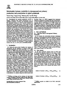
THE RELATIONSHIP BETWEEN SENSITIVITY AND VARIABILITY IN NORMAL AND GLAUCOMATOUS VISUAL FIELDS DAVID B. HENSON, SHAILA J. CHAUDRY and PAUL H. ARTES Department of Ophthalmology, University of Manchester, Manchester, UK

Abstract Purpose: To establish the relationship between sensitivity and variability in normal, ocular hypertensive and glaucomatous eyes. Method: Frequency-of-seeing (FOS) data were collected from four visual field locations of 64 eyes (22 normal, six ocular hypertensive and 38 glaucomatous), using a constant stimulus method on a Henson 4000 perimeter. At each location, 20 stimuli (0.5°) were presented (200 msec) at each of six intensities straddling the estimated threshold. In glaucomatous eyes, at least one location was chosen to lie in an area of normal sensitivity. The FOS data were fitted with a cumulative normal distribution, the standard deviation (SD) of which was used as an estimate of response variability. Results: Variability was found to increase with decreased sensitivity. The relationship was best described by the function loge(SD) = a * sensitivity(dB) + b, where the constants a and b were -0.08 and 3.22, respectively. Conclusions: Previously presented linear models of the relationship between sensitivity and variability fail to accurately predict variability at high and low perimetric sensitivities, suggesting negative variability at high sensitivities and underestimating variability at low dB values. Our model attempts to correct these shortcomings. It can be used in computer simulations of perimetry to estimate the performance of both existing and new perimetric algorithms.

Background An important parameter in the development and assessment of perimetric algorithms is the relationship between sensitivity and variability. Variability has been known for some time to increase when sensitivity reduces1-7. The magnitude of the effect can be very large; in areas of moderate sensitivity loss (8-18dB), the 95% confidence intervals can exceed the measurement range of the Humphrey Visual Field Analyzer8. Early research used repeat measures of the threshold to quantify variability (fluctuation), but more recent research has concentrated upon the use of frequency-of-seeing (FOS) curves9-13. The slope of the FOS curve gives a measure of response variability, while the 50% seen level gives a measure of sensitivity. FOS curves fully define the Address for correspondence: D.B. Henson, PhD, Department of Ophthalmology, University of Manchester, Royal Eye Hospital, Oxford Road, Manchester M13 9WH, UK

Perimetry Update 1998/1999, pp. 95–101 Proceedings of the XIIIth International Perimetric Society Meeting, Gardone Riviera (BS), Italy, September 6–9, 1998 edited by M. Wall and J.M. Wild © 1999 Kugler Publications, The Hague, The Netherlands back

54.p65

95

12/1/99, 11:02 AM

96

D.B. Henson et al.

stimulus response relationship and can be used in simulations to predict the performance of perimetric test algorithms. The relationship between FOS-derived measures of sensitivity and response variability has been reported by Weber and Rau9, Olsson et al.10 and Chauhan et al.11. Weber and Rau9 measured variability in normal eyes (central and peripheral locations) and in glaucomatous eyes. They found that a straight line could fit all their results with normal central locations at one end and defective glaucomatous locations at the other. Chauhan et al.11, while demonstrating a similar relationship, emphasized the poor quality of the linear fit at lower sensitivities. Olsson et al.10 found a good relationship between loge(variability) and threshold, pointing out that this transformation of the variability scale made the residuals reasonably independent of the variability. We re-visited the relationship between sensitivity and variability and concluded that the relationship is best expressed by a model where log (variability) is a linear function of sensitivity.

Method Subjects Data were collected from one eye of 22 normal subjects (median age 33, range 19-71 years), six ocular hypertensives (OHT) (median age 69.4, range 66-83 years), and 36 patients with primary open-angle glaucoma (POAG) (median age 67.5, range 33 to 80 years). Normal subjects were recruited from hospital staff, had no history of ophthalmic disease, a normal ophthalmic examination, no systemic illness, and a visual acuity better than 6/9. The OHTs were recruited from the glaucoma clinics at the Manchester Royal Eye Hospital. Inclusion/exclusion criteria were the same as for the normal subjects with the exception of a raised IOP. The POAG patients were also recruited from the glaucoma clinics at Manchester Royal Eye Hospital. They all had a confirmed diagnosis of POAG with visual field loss, stable controlled IOP, no other ocular pathology, previous experience with automated perimetry, and a visual acuity of better than 6/18. Test locations FOS data were collected at four visual field locations during a single experimental session. For the normal and ocular hypertensive subjects, the locations were 12.7° from fixation along the 45, 135, 225 and 315 meridians. For the glaucoma patients, one location was chosen to be in an area of normal sensitivity, and, if possible, three locations in or adjacent to a damaged area of the visual field. The damaged locations were chosen on the basis of a Humphrey Visual Field Analyzer (Program 24-2) test performed prior to the collection of FOS data. Data collection A computer program was specifically written to allow the collection of FOS data on a Henson 4000 bowl perimeter14. All stimuli subtended 0.5° and were presented for 200

54.p65

96

12/1/99, 11:02 AM


97

msec with a maximum luminance increment of 1000 cd/m5. After specification of the test locations, the program estimated the sensitivity at each location using the standard full threshold (4-2) strategy. For each location the program then selected five intensities which straddled the estimated threshold in 2dB steps. During each session, the experimenter, who received continuous feedback on the selected intensities and current responses, would repeatedly adjust the intensities and number of presentations to ensure that 1. the response range approached 0 and 100% seen; 2. data were collected for at least six intensities; and 3. there were a minimum of 20 presentations at each intensity. While the adjustments were being made, the subject was allowed a short rest. The presentation of stimuli was randomized with the inclusion of false positive and false negative response trials. Data analysis The FOS data from each test location were imported into the statistical package SPSS for probit regression analysis. The standard deviation (SD) of the fitted cumulative normal function was used as an estimate of response variability.

Results and discussion Figure 1 gives typical FOS data from one location in a normal eye (a) and two locations in a glaucomatous eye (b and c), one of which is from an area of reduced sensitivity (c). It can be seen that, while the data from the glaucomatous eye’s location with normal sensitivity are similar to that from the normal eye, the location with reduced sensitivity has a much shallower curve. When deciding upon appropriate test locations for the POAG eyes, one location was chosen to lie in an area of near normal sensitivity while the other three were chosen to lie in areas of reduced sensitivity. Many of the reduced sensitivity locations were subsequently found to yield results that, due to limitations in the dynamic range of the perimeter, did not approach the 100% seen level and could not, therefore, be accurately fitted by the probit function. These locations have not been included in the subsequent analysis. As sensitivity decreases, there is an increase in response variability (Fig. 2). This finding is in agreement with the earlier work of Weber and Rau9, Olsson et al.10 and Chauhan et al.11. The data also show an increased scatter of SD values with reduced sensitivity, a finding that was also noted by Chauhan et al.11. A linear fit to the data of Figure 2 underestimates variability at high and low sensitivities. It also predicts negative variability at high sensitivity, which is clearly at odds with common sense. The data in Figure 2 also show inequality of variance that violates the assumptions of the least-squares method. Figure 3 gives the same data after a log transform of the SD values as proposed by Olsson et al.10. The solid line (least-squares linear regression) now accurately represents the data. The parameters of the model loge(SD) = a * sensitivity + b were B0.08 and 3.22, respectively. Parameter b is dependent upon the decibel scale of the instrument. This model no longer predicts negative response variability at high sensitivities. The data points are now normally distributed around the regression line with equality of variance. The equation of the best linear fit to these data has been transformed and superimposed upon the data in Figure 2. The relationship between sensitivity and variability while being similar to that of Weber

54.p65

97

12/1/99, 11:02 AM

98

D.B. Henson et al.

Fig. 1. Three frequency-of-seeing curves. a. Normal eye; b. glaucomatous eye normal sensitivity; and c. glaucomatous eye reduced sensitivity.

54.p65

98

12/1/99, 11:02 AM


99

Fig. 2. Variability versus sensitivity linear axes.

Fig. 3. Variability versus sensitivity.

and Rau9 is much tighter than that reported by Chauhan et al.11. This can, in part, be explained by differences in experimental methods. Weber and Rau9 and the present research presented a fairly large number of stimuli at each intensity (25 and 20), while Chauhan et al.11 only presented five. With only five presentations, the precision of any FOS estimate is low, and even single response errors can result in large differences of the fitted function. Another difference in the methodology is that Weber and Rau9 and Chauhan et al.11 collected data at a greater number of stimulus intensities (ten and 17 versus a minimum of six in the present research). A large number of stimulus intensities leads to an increase in test time and invariably results in several test intensities with response probabilities close

54.p65

99

12/1/99, 11:02 AM

100

D.B. Henson et al.

to zero or one, which contribute little to the estimate of the FOS curve. For maximum information on the gradient of the FOS curve, data need to be collected at the shoulder areas of the curve. The technique used in this study allowed the operator to adjust the number of presentations and the intensities during the test. This ensured that most of the data were collected at intensities with high informational value and, thereby, contributed more to the accuracy of the FOS estimates. The more efficient approach adopted in the present research also meant that FOS curves could be determined from four visual field locations with a total number of presentations similar to that of a 30-2 full threshold test. As one of the intentions of the present research was to derive a relationship between sensitivity and response variability which could be used in perimetric simulations, it was felt important that as many parameters as possible, in particular test time, should be similar to those of a standard perimetric test. The data from normal, OHT and POAG subjects in Figures 2 or 3 are well described by a single model. There is no evidence of increased response variability for visual field locations of normal sensitivity in glaucomatous subjects. Our normal subjects with very high sensitivities showed an increase in their response variability. This might be due to frequent false-positive response errors that would lead to both an overestimation of sensitivity and to higher response variability. The present research has demonstrated that the relationship between sensitivity and log response variability can be well expressed by a linear function for normal, OHT and POAG eyes. This finding will be useful in computer simulations of perimetry to estimate the performance of both existing and new perimetric algorithms15.

Acknowledgments Supported by the International Glaucoma Association, Guide Dogs for the Blind and the Manchester Royal Eye Hospital endowment funds.

References 1. Holmin C, Krakau CET: Variability of glaucomatous visual field defects in computerised perimetry. Graefe’s Arch Exp Ophthalmol 210:235-250, 1979 2. Werner E, Saheb N, Thomas D: Variability of static threshold responses in patients with elevated IOPs. Arch Ophthalmol 100:1627-1631, 1982 3. Flammer J, Drance S, Zulauf M: Differential light threshold; short and long term fluctuation in patients with glaucoma, normal controls, and patients with suspected glaucoma. Arch Ophthalmol 102:704-706, 1984 4. Wilensky JT, Joondeph BC: Variation in visual field measurements with an automated perimeter. Am J Ophthalmol 97:328-331, 1984 5. Katz J, Sommer A: Asymmetry and variation in the normal hill of vision. Arch Ophthalmol 104:65-68, 1986 6. Lewis RA, Johnson CA, Keltner JL, Labermeier PK: Variability of quantitative automated perimetry in normal observers. Ophthalmology 93:878-881, 1986 7. Heijl A, Lindgren G, Olsson J: Normal variability of static perimetric threshold values across the central visual field. Arch Ophthalmol 105:1544-1549, 1987 8. Heijl A, Lindgren A, Lindgren G: Test-retest variability in glaucomatous visual field. Am J Ophthalmol 108:130-135, 1989 9. Weber J, Rau S: The properties of perimetric thresholds in normal and glaucomatous eyes. German J Ophthalmol 1:79-85, 1992

54.p65

100

12/1/99, 11:02 AM


101

10. Olsson J, Heijl A, Bengtsson B, Rootzen H: Frequency-of-seeing in computerised perimetry. In: Mills RP (ed) Perimetry Update 1992/1993, pp 551-556. Amsterdam/New York: Kugler Publ 1993 11. Chauhan B, Tompkins J, LeBlanc R, McCormick T: Characteristics of frequency-of-seeing curves in glaucoma in normal subjects, patients with suspected glaucoma, and patients with glaucoma. Invest Ophthalmol Vis Sci 34:3534-3541, 1993 12. Henson DB, Evans J, Chauhan BC, Lane C: Influence of fixation accuracy on threshold variability in patients with open angle glaucoma. Invest Ophthalmol Vis Sci 37:444-450, 1996 13. Wall M, Maw R, Stanek K, Chauhan B: The psychometric function and reaction times of automated perimetry in normal and abnormal areas of the visual field in patients with glaucoma. Invest Ophthalmol Vis Sci 37:878-885, 1996. 14. Henson DB: A look at the new Henson perimeter. Optician 206:17-20, 1993 15. Henson DB, Artes PH, Chaudry SJ, Chauhan B: Suprathreshold perimetry: establishing the test intensity. This Volume, pp 243-252

54.p65

101

12/1/99, 11:02 AM