DECEMBER 2004
1895
MITCHELL ET AL.
The Residual GEM Technique and Its Application to the Southwestern Japan/East Sea D. A. MITCHELL,* M. WIMBUSH,
AND
D. R. WATTS
Graduate School of Oceanography, University of Rhode Island, Narragansett, Rhode Island
W. J. TEAGUE Naval Research Laboratory, Stennis Space Center, Mississippi (Manuscript received 9 September 2003, in final form 25 March 2004) ABSTRACT The standard gravest empirical mode (GEM) technique for utilizing hydrography in concert with integral ocean measurements performs poorly in the southwestern Japan/East Sea (JES) because of a spatially variable seasonal signal and a shallow thermocline. This paper presents a new method that combines the U.S. Navy’s Modular Ocean Data Assimilation System (MODAS) static climatology (which implicitly contains the mean seasonal signal) with historical hydrography to construct a ‘‘residual GEM’’ from which profiles of such parameters as temperature (T ) and specific volume anomaly (d) can be estimated from measurements of an integral quantity such as geopotential height or acoustic echo time (t). This is called the residual GEM technique. In a further refinement, sea surface temperature (SST) measurements are included in the profile determinations. In the southwestern JES, profiles determined by the standard GEM technique capture 70% of the T variance and 64% of the d variance, while the residual GEM technique using SST captures 89% of the T variance and 84% of the d variance. The residual GEM technique was applied to optimally interpolated t measurements from a two-dimensional array of pressure-gauge-equipped inverted echo sounders moored from June 1999 to July 2001 in the southwestern JES, resulting in daily 3D estimated fields of T and d throughout the region. These estimates are compared with those from direct measurements and good agreement is found between them.
1. Introduction The gravest empirical mode (GEM) technique is a method for determining oceanic vertical profiles from vertically integrated quantities. Historical hydrography is used to calculate characteristic relationships for temperature (T), salinity (S), and specific volume anomaly (d) as functions of pressure (p) and a vertically integrated quantity, such as acoustic echo time (t, used here), geopotential height (f), or heat content. These relationships (when they exist) form lookup tables known as the GEM fields, denoted as TG (p, t), SG (p, t), and d G (p, t) (Meinen et al. 2002), respectively. As a result, a single inverted echo sounder (IES) t measurement, satellite altimeter sea surface height measurement, or expendable bathythermograph (XBT) determination of heat content can provide an estimate of full vertical profiles of T, S, and d when combined with the appropriate GEM fields. * Current affiliation: Naval Research Laboratory, Stennis Space Center, Mississippi. Corresponding author address: Dr. Douglas A. Mitchell, Department of the Navy, Naval Research Laboratory, Code 7332, Stennis Space Center, MS 29529-5004. E-mail:
[email protected]
q 2004 American Meteorological Society
Two requirements must be met in order for the GEM method to be successful. They are, as stated by Meinen et al. (2002), that ‘‘there must be sufficient hydrography within the study region to characterize the mesoscale variability, and the temperature–salinity relationship must be temporally stable [along each streamline] but not necessarily tight [across streamlines]’’ (see also Watts et al. 2001). The second requirement can be restated as follows: there must be a nearly one-to-one relationship between t and the corresponding vertical profile of interest. What we mean by ‘‘nearly one-toone’’ is that there must be a general grouping of similar profiles about a particular t; that is, each of the profiles having t values within a small range of a particular t must be similar within an acceptable amount of scatter. The GEM technique was first developed by Meinen and Watts (2000) to study the vertical structure and transport of the North Atlantic Current. It has also been used successfully to investigate the Subantarctic Front (Watts et al. 2001), the Antarctic Circumpolar Current (Sun and Watts 2001), and the development of small meanders in the Kuroshio (Book et al. 2002). Each of these study regions have in common two important properties: 1) strong baroclinic variability extending to pressure levels of 1000 db (1 db 5 10 5 Pa) or more, resulting in the baroclinic signal being much larger than
1896
JOURNAL OF ATMOSPHERIC AND OCEANIC TECHNOLOGY
VOLUME 21
FIG. 1. The PIES locations in the southwestern JES are shown (black triangles). Bathymetry is shaded where darker shades represent shallower depths. The black dots represent the locations of the 2248 historical hydrocasts (many locations have repeat measurements) to at least 500-m depth, used to calculate the residual GEM fields. PIES sites P32 and P4-1 were not recovered.
the seasonal signal; and 2) disparate hydrographic vertical profiles producing distinct t values. These two similarities result in ‘‘well ordered’’ relationships between t and the vertical structures of T, d, etc., which are required for the standard GEM technique to perform satisfactorily. In the above GEM studies, which captured greater than 90% (and as much as 97%) of the variance in T and d below the penetration depth of the seasonal signal (100–300 m depending on the region), the authors used various estimates of the seasonal signal to improve the GEM’s performance in the seasonally varying upper layers. Meinen and Watts (2000) applied a simple seasonal correction only to the hydrographic and pressuregauge-equipped inverted echo sounder (PIES) t values but did nothing to seasonally correct the T data. Watts et al. (2001) developed an empirical model of the annual march of T, S, d, and t, which resulted in about a 30% reduction in rms error of the T estimates for the upper100-db layer. Book et al. (2002) developed seasonal estimates for T, d, and t using an iterative approach similar to that of Watts et al. (2001). Despite these efforts, significant variance remained uncaptured in the upper 100–200 m. Three possible reasons for this uncaptured variance are 1) spatial variation of the mean
seasonal signal within the study region, 2) interannual variation in the shape and amplitude of the seasonal signal, and 3) short-term atmospheric effects. In any case, most of the variability in geopotential height in these study regions occurs below the upper 100–300 m due to the strong baroclinicity that extends to pressure levels greater than 1000 db. Therefore, the error associated with the upper few hundred meters was considered acceptable for their analyses. The standard GEM technique performs poorly when applied to the Ulleung Basin (UB) of the southwestern Japan/East Sea (JES) (Fig. 1) for two reasons: a shallow permanent thermocline and a spatially variable seasonal signal (Fig. 2 and Fig. 3, left panel). Normally, a representative seasonal signal for a region calculated from hydrography (using one of the methods mentioned above) is removed from the data prior to calculation of the GEM fields. In the UB the permanent thermocline is only 50–250 m deep, and hence the seasonal signal fundamentally alters its structure. Moreover, even within this limited region, the seasonal signal varies in vertical structure, amplitude, and phase from one location to another. Thus, it was determined that the calculation of a single seasonal signal to represent the entire UB was unacceptable. Efforts to calculate seasonal signals for
DECEMBER 2004
MITCHELL ET AL.
1897
FIG. 2. The seasonal signal as seen in the MODAS static climatology in the southwestern JES. The four left-hand panels show the temperature at 100 m in Feb, May, Aug, and Nov. The rightmost panel shows vertical profiles for the same four months. The solid lines represent the location depicted by the diamonds in the four left-hand panels, and the dashed lines represent the location depicted by the squares in those panels. The numbers at the top of the panel indicate the month during which the profile was taken.
subregions were not made because there were insufficient data to resolve the seasonal signal, because good temporal coverage of the hydrographic data only occurred in a few localized areas. The difficulties involved are illustrated in Fig. 3 with four temperature profiles, the two on the left for winter and summer at a single location and the two on the right for different locations in the same month. All four profiles have essentially the same t value yet have very different shapes: in two, the surface layer is warm and the thermocline is shallow and cool; in the other two, the surface layer is relatively cool and depresses the thermocline, making it relatively warm. For a given t value, relatively warm temperatures in one layer must be compensated by relatively cool temperatures in another. The limitations of the standard GEM technique are most clearly illustrated in the right-hand panel. Since the two profiles occur in the same month and have essentially the same t, the standard GEM, even with a seasonal correction (i.e., Watts et al. 2001 or Book et al. 2002), could only produce a single estimate for these
two profiles. On the other hand, the new technique described in this paper (and as shown in Fig. 3) produces a different and improved estimate for each of these profiles. The standard T GEM field for the Ulleung Basin and its associated rms error is shown in Fig. 4. The GEM field clearly illustrates that the thermocline and strong baroclinicity resides between 50 and 250 m throughout the UB. The bottom panel highlights the error above the thermocline associated with the seasonal signal, with a mean error in the upper 100 db of 2.78C and a maximum error of 5.68C. Thus, we found the error associated with the seasonal signal unacceptably large. Interestingly, for short travel times (i.e., 0.670–0.673 s) there is a local minimum in the error field that resides near 200 m for t 5 0.670 s and rises to 170 m for t 5 0.673 s. This occurs because disparate T profiles contribute to the GEM at similar t (e.g., Fig. 3), indicating that the second GEM requirement described above is not being satisfied. The GEM technique depends solely on the correlation
1898
JOURNAL OF ATMOSPHERIC AND OCEANIC TECHNOLOGY
VOLUME 21
FIG. 3. (left) Hydrographic temperature profiles near 36.368N, 134.088E for Mar and Aug, illustrating the seasonally changing vertical structure. (right) Hydrographic temperature profiles for two locations 325 km apart during Feb. In each panel, two measured temperature profiles (solid lines) with similar t values are compared with profiles estimated from the standard GEM technique (dashed line) and with the residual GEM technique (thin solid lines with dark circles).
between the parameterization variables (t and p, in this case) and the variables of interest (T, S, d, etc.). Since t is determined by sound speed (c), which depends strongly on T, one might expect a T GEM to perform well. However, a T GEM only performs well when the vertical distribution of T, that is, T(p), is strongly related to t. In the JES, their relation was too weak to allow accurate estimates of T(p), thus leading us to seek an improved method. This new method, the residual GEM technique, works well because T9(p) and t 9 (where a prime indicates the residual value after removal of the climatological value) are strongly related [as are d9(p) and t 9]. Unfortunately, neither S(p) and t, nor S9(p) and t 9, are strongly related in the JES. Therefore, the remainder of this paper will examine T and d only. The purpose of this paper is to document a new technique, referred to as the residual GEM technique, designed to address the above problems. We use a spatiotemporal climatology to represent the seasonal signal, and t measurements to estimate residual differences from that climatology. Hence, we call it the residual GEM technique.
2. Methods a. Data used to calculate residual GEMs The U.S. Navy’s Modular Ocean Data Assimilation System (MODAS) static climatology fields (Fox et al. 2002) for T and S for the JES are provided bimonthly starting in January (on the 15th), on a 1⁄8 3 1⁄8 grid at 37 depth levels from 0 to 6500 m. The vertical profiles were linearly interpolated from 0 to 500 db in 10-db increments for direct use with the GEM technique. Extraction of a MODAS climatological profile for a particular location and time is done through bilinear interpolation in the horizontal, and linear interpolation in time. A set of 2248 historical hydrocasts from the Korean Oceanographic Data Center, Japan Oceanographic Data Center, and Hydrobase (Macdonald et al. 2001) for the region 35.58–408N by 1298–1368E was used in determining the residual GEMs. This region, which is approximately 4 times as large as the deployed PIES array, was chosen because it was the smallest region that contained sufficient hydrography to characterize the mesoscale variability, thus satisfying the first requirement
DECEMBER 2004
1899
MITCHELL ET AL.
FIG. 4. (top) The standard temperature GEM lookup table. (bottom) The standard temperature GEM’s rms error field. Note the different scales.
of the GEM technique. The casts span the years 1930– 96 and are broadly distributed seasonally, interannually, and spatially across the southern JES (Fig. 1). Sea surface temperature (SST) data were provided by Remote Sensing Systems as daily 3-day averages and weekly composites on a 0.258 3 0.258 grid covering the full UB. These data were collected by the Tropical Rainfall Measuring Mission (TRMM) Microwave Imager, which is a satellite-borne multichannel scanning passive microwave radiometer designed to observe precipitation (Quartly and Srokosz 2002). Its 10.7-GHz channel collects SST data through nonprecipitating clouds. Since the SST values near land are contaminated by the land, the coastal grid locations were filled with MODAS climatological values. Missing values caused by precipitation were handled in one of two ways. First, if there were fewer than 10 missing values on any given daily map, those values were filled in with interpolated values from neighboring points. Second, if there were 10 or more missing values, they were replaced with the weekly composite values. b. Development of residual GEM fields In the residual GEM technique (for t) first we calculate
tp 5 2
E 0
p
dp˜ , rg0 c
where p is a chosen pressure level, r is density, we assume constant gravity g 0 5 9.8 m s 22 , and c is the speed of sound (see Meinen and Watts 1997) both for the hydrocasts and for the MODAS profiles. Residual values were calculated as
x9 5 x 2 xMODAS , where x are the hydrocast values (T, SST, d, or t) and xMODAS are the corresponding MODAS values interpolated to the CTD sites and times of year. Hereafter the procedure follows the (standard GEM) discussion of Watts et al. (2001). How the residual T and d GEM fields were empirically fitted to the data is illustrated in Fig. 5. The upper four panels in Fig. 5 are scatterplots of T9 versus t 9 [p 5 500 db is used (Mitchell et al. 2004) here and throughout], and the lower four panels are scatterplots of d9 versus t 9 at representative pressure levels. At each pressure level, the residual (either t 9 or d9) displays a functional relationship (plus scatter) with t 9. The curve superimposed on each plot is a smoothing cubic spline curve fit to the data. The degree of smoothing (‘‘spline tension’’) is the same at all levels, such that the rms error approximately matches the a priori
1900
JOURNAL OF ATMOSPHERIC AND OCEANIC TECHNOLOGY
VOLUME 21
FIG. 5. The upper four panels show the residual temperature (T 9) vs t 9500 at the surface and at 100, 200, and 300 db. The superimposed lines are the smoothed GEM curves fit to the data. The lower four panels are the same, but for d.
DECEMBER 2004
MITCHELL ET AL.
error, which is defined as the zero limit of the structure function calculated from these data (Willeford 2001). A cubic spline curve under tension was fitted to the T9 versus t 9 data and to the d9 versus t 9 data at each 10-db level between 0 and 500 db. This procedure produced 51 spline curves for both T9 and d9, with a unique T9 and d9 for each (t 9, p) pair, denoted by T9G(t 9, p) and d9G(t 9, p). These parameters were contoured as the two-dimensional ‘‘GEM fields’’ shown in Fig. 6 (first and third panels). Notice that the d9 GEM closely resembles the T9 GEM in pattern, suggesting that variations in the density field are determined primarily by T variations. The rms T and d error fields from the residual GEM are also shown in Fig. 6 (second and fourth panels). The mean error in the upper 100 db of the residual T GEM was 1.68C with a maximum error of 2.28C near 50 db. The depth to which the error penetrates closely follows the thermocline depth. As seen in the standard GEM rms error field (Fig. 4, bottom panel), a local minimum in the error field resides near 200 m for t 5 0.670 s and rises to 170 m for t 5 0.673 s. However, the magnitude of the error associated with this feature has been reduced by about 30%, indicating that the residual GEM technique has reduced the variability associated with this feature but has not removed it completely. For notational brevity, we will refer to this feature as MVS, which is short for multiple vertical structures for similar t. Interestingly, the MVS is not present in the d rms error field, indicating that S variations are correlated with T variations; that is, warmer waters are saltier and cooler waters are fresher. Thus, the density field is less affected by MVS than the T field. In contrast to Fig. 5, which shows horizontal slices through the T9 GEM field, Fig. 7 (top panel) shows vertical slices through the T9 GEM field at five discrete t 9 values. The thick, green curves are T9G (t 9, p) at each respective t 9. Grouped about each of these curves are all of the hydrographic T9(p) measurements within 60.15 ms of the respective t 9 values. The consistency of T9(p) profiles when grouped by t 9 from hydrographic data spanning 66 yr and all seasons confirms the effectiveness of parameterizing T9(p) with t 9. The vertical structure of the residual GEM field (the corrector, where MODAS is the predictor) changes substantially between groupings, from a 175-db, 68C warm correction at one extreme to a 75-db, 288C cold correction at the other. This indicates that negative residuals (t , tMODAS ) require a deepening of the thermocline and positive t residuals require a shoaling of the thermocline. Below 300 db their structure is nearly indistinguishable, displaying the near homogeneity of the waters below the shallow thermocline. Histograms of t from the 2248 hydrocasts used to construct the residual GEMs (Fig. 6, fifth panel) and t from the PIES measurements (Fig. 6, bottom panel) indicate that the MVS structure is relatively rare. The region of MVS, defined as the region where the local
1901
minimum rms error at 180 db is at least 0.58C less than the surrounding two maximum rms error regions, occurs for values of t 9 , 22.5 ms, and these account for less than 12% of the profiles used in the construction of the residual GEMs and less than 4% of the t measurements collected by the PIES array. Therefore, these profiles exert little influence over the results presented below. c. Residual GEM technique advantages The residual GEM technique is a predictor/corrector technique in which suitable climatological profiles are the predictors and the residual GEM fields are the correctors. We chose to use the MODAS static climatology (Fox et al. 2002) as the predictor, because it offers higher horizontal resolution in the JES than other available climatologies. MODAS offers two advantages in the JES that address the reasons for the poor performance of the standard GEM technique described above: 1) MODAS is a 4D climatology (x, y, z, t) that implicitly contains the regionally variable seasonal signal, and 2) MODAS incorporates the mixture of shallow thermocline and seasonal signal. Increased accuracy of the residual GEM technique compared with the standard GEM technique, for profiles that the standard GEM technique estimated poorly for the reasons discussed earlier, are shown in Fig. 3. When computing GEMs by the residual GEM technique, residual profiles are created by removing the temporally and spatially interpolated MODAS climatological profiles from the measured hydrographic profiles. The variability of the residual profiles is less than the variability of the original hydrographic profiles; accordingly, errors associated with estimating these profiles with a GEM field are also reduced. The residual GEM fields, which are the correctors, address nonseasonal (interannual and mesoscale) variability. d. Further parameterization by SST9 The rms error fields for the residual GEM technique (Fig. 6, second and fourth panels) indicate that there is still significant error in the surface layers. Since the residual GEM technique conserves t 9, and thus heat content, errors in the residual GEM estimate of T and d anywhere in the water column result in compensating errors somewhere else in the water column. Thus, any additional information about the heat content of the water column can be used to constrain and improve the residual GEM estimates. During the deployment of the PIES array, the only other relevant data collected concurrently over the entire PIES array were satellite-measured SST data (described above). Therefore, we further improve the residual GEM by additional parameterization with SST9, that is, T(x, y, p, t) 5 TMODAS (x, y, p, t) 1 T9G(p, t 9, SST9). Three SST9 bins were selected based on two factors: 1) the rms difference between the estimated profiles and the historical profiles is minimized, and 2) the distributions of SST9 and t 9 ensure the GEM
1902
JOURNAL OF ATMOSPHERIC AND OCEANIC TECHNOLOGY
FIG. 6. (top panel) The residual temperature GEM T9GEM (p, t 9500 ). (second panel) The rms difference between the residual-GEM-estimated T profiles and the 2248 hydrocasts used to construct the residual GEM. (third panel) The residual d GEM dGEM 9 (p, t 9500 ). (fourth panel) The rms difference between the residual-GEM-estimated d profiles and the 2248 hydrocasts used to construct the residual GEM. (fifth panel) Distribution of t 9500 used to construct the residual GEMs. (bottom panel) Distribution of t 9500 as measured by the PIES.
VOLUME 21
DECEMBER 2004
MITCHELL ET AL.
FIG. 7. (top panel) Five groupings of temperature profiles, each showing all the profiles from the 2248 profiles used to construct the residual GEMs that are within 60.15 ms of the five central t 9500 values as labeled in the bottom panel. The green curves are the corresponding T9G profiles at each of the same five t 9500 values. The leftmost set of profiles has no offset, and each successive curve is offset 128C from its predecessor. (second panel) Same as the top panel, except only those profiles with an SST9 value less than 218C are plotted. The leftmost grouping has no T 9 curves plotted, indicating that profiles with fast t 9500 values (i.e., negative values) rarely occur when the sea surface is cooler than climatological values. (third panel) Same as the top panel, except only those profiles with SST9 values greater than 218 and less than 28C are plotted. (bottom panel) Same as the top panel, except only those profiles with SST9 values greater than 28C are plotted. The rightmost grouping has no T 9 curves plotted, indicating that profiles with slow t 9500 values (i.e., positive values) rarely occur when the sea surface is warmer than climatological values.
1903
1904
JOURNAL OF ATMOSPHERIC AND OCEANIC TECHNOLOGY
VOLUME 21
resembles that of T. It also increases from the surface to 50 db before steadily decreasing: it is less than 0.598 3 10 27 m 3 kg 21 below 250 db, less than 1.39 3 10 27 m 3 kg 21 below 130 db, and less than 3.92 3 10 27 m 3 kg 21 in the highly variable seasonal thermocline. The relatively high error in d near the surface results from large-amplitude (;3 psu) variations in S, which create changes in d that are not well correlated with t. All further discussion, unless explicitly noted, refers to the residual GEM technique with SST9 parameterization. e. Residual GEM field interpretation
FIG. 8. Standard deviation of Tmeasured 2 Testimated for the standard GEM technique (dashed–dotted line), the residual GEM technique (dashed line), and the residual GEM technique with SST9 parameterization (solid line).
structures are well represented in parameter space. The bins selected were SST9 , 218C (bin 1), 218C , SST9 , 28C (bin 2), and SST9 . 28C (bin 3). Residual GEM fields, one for each SST9 bin, were then calculated as described above for T and d. The rms error in the upper 100 db (not shown) was 1.448C with a maximum error of 2.148C. The vertical T profiles along with the residual-GEMestimated T profiles (thick green lines) for the three SST9 bins for profiles within 60.15 ms of the labeled t values are shown in Fig. 7 (lower three panels). The negative t 9 (i.e., warm correction) T G estimates have similar structures between 50 and 500 db for all three SST9 bins, with the main differences confined to the top 50 db. The positive t 9 estimates (i.e., cold correction) display a marked change between the surface and 300 db. In particular, the maximum correction at 100 db changes by about 28C, with the largest correction occurring for the greatest SST9. Thus, as expected, a warming/cooling at the sea surface requires a cooling/warming of the subsurface to conserve t. The standard deviation of the error for the standard GEM technique, the residual GEM technique, and the residual GEM technique with SST9 parameterization are shown in Fig. 8. The residual GEM technique (dashed line) offers a significant improvement over the standard GEM technique (dashed–dotted line), and parameterization by SST9 (solid line) shows further improvement, particularly in the top 50 db. The rms error in estimated T increases from the surface to 50 db, after which it steadily decreases: it is less than 0.68C below 250 db, less than 18C below 130 db, and less than 1.78C even in the highly variable seasonal thermocline (upper 100 db). The rms error in estimated d (not shown) closely
The 2D residual GEM fields act as corrector lookup tables to MODAS climatological predictions. The MODAS predictor profiles TMODAS (x, y, p, t) contain the basic spatial and temporal information, and the corrector T9G(p, t 9) profiles make first-order corrections based on t 9. Figure 9 shows a suite of T9G profiles that correspond to chosen t 9 values at 0.002-s intervals for the center SST9 bin. Each of the 23 PIES, during the 2-yr measurement period, experienced the full range of t 9 values plotted here. The error bars are the rms-associated deviations of T9 (obtained from the hydrographic measurements) from the corresponding T9G value; these indicate the uncertainty in T profiles determined by the residual GEM technique from a precise measurement of t. The magnitude of the largest error bars below the surface (61.58C), being an order of magnitude smaller than the temperature change across the suite of curves (;148C), shows that the error associated with individual temperature corrections is much less than the range of corrections employed. Therefore, the residual GEM technique is a useful tool for tracking changing water column properties. The residual GEM fields give information about how the water column differs from the MODAS static climatology. For example, the T9G field (Fig. 6) shows how for a negative t 9 value (i.e., measured t less than climatological t for a given location) a particular warmanomaly profile must be added to the climatological profile to produce the proper t. Likewise, a cold-anomaly profile must be added for a positive t 9 value. Of course, the residual GEM fields must be recombined with the MODAS profiles, that is, T(x, y, p, t) 5 TMODAS (x, y, p, t) 1 T9G(p, t 9, SST9), in forming an estimate of the water column temperature profile. The standard deviations of T and d and the percent variance captured by the T9 and d9 residual GEM fields as a function of pressure are shown in Fig. 10. For both parameters, the peak standard deviation and its associated minimum in the captured percent variance occur near 50 db. This happens because the mixed layer depth, which displays strong nonseasonal variation, may be incorrectly estimated by the residual GEM technique. Since the thermocline in this region is shallow and marked by a strong vertical gradient below the mixed
DECEMBER 2004
MITCHELL ET AL.
1905
FIG. 9. Suite of five T9G curves for labeled t 9 values for the center SST9 bin (218C , SST9 , 28C). The error bars are the associated rms error values.
layer, the incorrect estimation of the mixed layer depth generates maximum error at the level where the gradient below the mixed layer is strongest on average for the UB. This occurs at 50 db in the UB and is the largest source of error in the residual GEM technique. Since the residual GEM technique conserves t, which is approximately proportional to integrated heat content, the over- or underestimation of the mixed layer depth results in compensatory under- or overestimation of the heat content of the profiles below the mixed layer. The residual GEM technique, which is based on an integrated quantity (t) that depends strongly on temperature, can be used to estimate other integrated quantities that depend on temperature. For example, heat content is readily determined from t, because the two are nearly linearly related. The residual GEM technique can also be used to estimate geopotential height relative to 500 db (f) (Fig. 11). The rms difference between residual-GEM-estimated f and that calculated directly from the 2248 hydrocasts used to calculate the GEM is 2.44 cm. The f values from the hydrocasts span a range of about 52 cm, from a minimum of about 37.5 cm to a maximum of nearly 90 cm. Therefore, the uncertainty in f relative to its full range is only about 5%.
3. Comparisons with other observations a. Data used in comparisons An array of 25 PIES was deployed during June 1999 as an approximate 5 3 5 array with 50–60-km spacing covering a 220 km 3 240 km region in the UB (Fig. 1), (Mitchell et al. 2004; Teague et al. 2004). The data were collected as components of the U.S. Office of Naval Research JES program. Twenty-three PIES were recovered in June–July 2001, with crab fishing probably responsible for the two losses. Instrument spacing was selected to allow coherent mapping of mesoscale features, based on a correlation length scale of 100 km estimated for upper-layer features using Rossby wave theory (Matsuyama et al. 1990). A PIES measures vertical acoustic travel time with an accuracy of 1.6 ms and a resolution of 0.1 ms (Chaplin and Watts 1984; Meinen and Watts 1998), abyssal pressure with an accuracy of 0.1–0.3 db and a resolution of 0.001 db (Watts et al. 2001), and temperature (used to correct the Digiquartz pressure transducer’s temperature sensitivity) with an accuracy of 0.158C and a resolution of 0.00078C. All measurements were recorded hourly.
1906
JOURNAL OF ATMOSPHERIC AND OCEANIC TECHNOLOGY
VOLUME 21
FIG. 10. (top left) Standard deviation of Tmeasured 2 Testimated for standard GEM (thin line) and residual GEM with SST9 parameterization (thick line). (top right) Same as top left, except for d. (bottom left) Percent of signal captured by the standard GEM (dashed line) and residual GEM with SST9 parameterization (thick line). (bottom right) Same as bottom left, except for d.
High-resolution CTDs from surveys conducted in the UB during the PIES deployment period were provided by K.-I. Chang of the Korean Oceanographic Research and Development Institute (KORDI). CTDs were also provided by the Korean Oceanographic Data Center (KODC). b. KORDI CTD data and KODC CTD data Independent confirmation of the residual GEM technique is accomplished by comparison with 27 CTD casts collected by KORDI and KODC within 2 km of PIES sites. These 27 CTDs were not used in the construction of the residual GEMs. The 2-km radius was chosen to limit the effects of spatial gradients between the CTD and PIES sites. To ensure a fair comparison, only CTD casts with t 500 values within 60.35 ms of the PIESdetermined t 500 value [PIES t measurements are linearly related to t 500 (Mitchell et al. 2004)] are considered (this excludes five CTD casts), because it allows the maximum number of CTD casts within the expected a priori error for t. The five excluded CTD casts occurred at times when the PIES t data were extremely noisy and
considered unreliable for accurate comparison. The difference in measured t between the PIES and the remaining 27 CTD values, apart from measurement uncertainty and noise (particularly in the PIES t measurements), occurs largely because of the smoothing effect of the 5-day low-pass filter applied to the PIES t measurement, while the CTD casts, which represent measurements taken over a short duration, may contain high-frequency information filtered out of the PIES data. The results of the comparisons are shown in Fig. 12. The main panels show the 27 CTD casts (solid lines) and the PIES-derived profiles (dashed lines) arranged by increasing rms difference. These profiles show that by under- or overestimation of the depth of the surface mixed layer by the residual GEM technique (as explained above) results in an error peak in the 30–50-db range. Furthermore, under- or overestimation of the mixed layer depth results in a compensating over- or underestimation of temperature deeper in the water column. The right-hand panel shows the standard deviation of the difference between the CTD and the PIES residual GEM values. It closely resembles the standard deviation of the residual T shown in Fig. 8 (leftmost curve), show-
DECEMBER 2004
MITCHELL ET AL.
1907
FIG. 11. (top) Geopotential height at the surface relative to 500 db arranged by ascending t, as measured by the 2248 hydrocasts (black dots) and as estimated by the residual GEM technique (green dots). (bottom) Geopotential height differences at the surface relative to 500 db: hydrocasts 2 residual GEM estimates. The red lines represent one standard deviation (62.44 cm).
ing that the residual GEM technique is performing within predicted limits. Figure 13 shows the difference in f between the 27 CTD casts and the PIES-derived values, arranged in the same manner as in Fig. 12. The rms difference is 2.07 cm, which is 15% less than the 2.44-cm expected value (Fig. 11). The magnitude of the largest difference in Fig. 13 is 5.45 cm (comparison 23). It is caused by anomalously low salinity in the upper 50 db (Fig. 14). The fact that this difference appears to be largely due to the departure of S from its climatological value can be demonstrated by calculating f for this CTD cast in two different ways: 1) calculate it with the CTD T and S profiles, which gives a value of 78.26 cm, and 2) calculate it with the CTD T profile and the MODAS climatological S profile, which gives a value of 72.88 cm. The difference between these two calculations is 5.38 cm, which accounts for 98.7% of the difference between the CTD-measured and PIES-measured f values for the significant outlier. A similar calculation for all 2248 hydrocasts used to construct the residual GEMs, that is, calculating f(S, T) and f(SMODAS , T), reveals that 70% of the error in the residual-GEM-estimated f is caused by uncorrelated S variations.
4. Summary and conclusions The standard GEM fields, though not as accurate as the residual-GEM-estimated fields, are still useful as a visual aid for gaining insight into the basic water properties and vertical structures present in a region. The traditional T GEM field (Fig. 4, top panel) clearly displays the shallow thermocline present throughout the UB. The associated rms error field (Fig. 4, bottom panel) highlights, by the larger error above 100 db, the need to remove a well-represented seasonal signal from the data prior to calculating the GEM field, at least in regions where the main thermocline is shallow. The technique described in this paper was developed to accomplish this in the UB. The residual GEM technique, which combines a suitable climatology with the GEM technique to quantify the water column characteristics of a region, was used to interpret data collected by an array of PIES in the JES. The U.S. Navy’s static MODAS climatology was used because of its increased horizontal resolution in the JES compared to other readily available climatologies. The residual GEM technique addresses two difficulties experienced by the standard GEM, a spatially
1908
JOURNAL OF ATMOSPHERIC AND OCEANIC TECHNOLOGY
VOLUME 21
FIG. 12. (main panels) Comparisons between 27 T profiles from the residual GEM technique (with SST9 parameterization) applied to PIES data (dashed lines) and from KORDI CTD casts (solid lines) taken within 2 km of the PIES sites and having t within 60.35 ms of the PIES determined values, arranged in order of increasing rms difference. (secondary panel) The rms difference between the PIES and CTD profiles.
FIG. 13. The rms difference between the geopotential height at the surface relative to 500 db (cm) from the 27 KORDI CTD casts in Fig. 12 and the PIES-derived values. The black lines represent the expected error of the residual GEM technique (62.44 cm).
FIG. 14. The KORDI CTD-measured salinity profile taken at 37.078N, 130.948E on 18 Oct 1999 (solid line) and the MODAS climatological estimate of the CTD profile (dashed line).
DECEMBER 2004
1909
MITCHELL ET AL.
varying seasonal signal and a shallow thermocline. The residual GEM technique, a predictor/corrector scheme, addresses these difficulties by using the MODAS climatology as the predictor, because MODAS implicitly contains the seasonal signal and the shallow thermocline. The residual GEMs, which are the correctors, address mesoscale variations by characterizing departures from MODAS as a function of acoustic echo time. As a further refinement, the residual GEMs are additionally parameterized by SST9, which reduces the errors near the surface. The residual GEM technique (with SST parameterization) captures 89% of the T variance and 84% of the d variance in the interval 0–250 db (i.e., within the thermocline). In the upper 100 db, where the seasonal signal exerts the most influence, the residual GEM technique reduces the rms error by about 47% compared to the standard GEM (from 2.78 to 1.448C). Comparisons of 27 high-resolution CTD casts taken within 2 km of PIES sites during the PIES deployment period with residual GEM T profile estimates (Fig. 12) reveal that the estimated profiles capture the dominant vertical structure of each of the CTD profiles. Integrated quantities, such as geopotential height of the surface relative to 500 db (f), are often well reproduced by the residual GEM technique. The standard deviation in f error computed from the standard GEM is 4.46 cm, while it is reduced to 2.44 cm with the residual GEM technique. It was further demonstrated that 70% of this uncertainty can be attributed to uncorrelated S variations. The residual GEM technique requires three criteria be met in order to perform well: 1) a strong relationship between a measurable integral quantity and a variable of interest, such as between t 9 and T9(p); 2) sufficient hydrography to characterize this relationship in the desired region; and 3) the availability of a robust climatology with adequate spatial and temporal resolution. In order to determine if a region is well suited to the GEM techniques, either standard or residual, the GEMs must be calculated and their errors determined based on available hydrography. Fortunately, once the available hydrography has been collected, calculating GEMs and determining their errors is quick and straightforward. Acknowledgments. This work was supported by the Office of Naval Research ‘‘Japan/East Sea DRI.’’ Basic Research Programs include the Japan/East Sea initiative under Grant N000149810246 and the Naval Research Laboratory’s ‘‘Linkages of Asian Marginal Seas’’ under Program Element 0601153N. The authors would like to
thank G. Chaplin, M. Mulroney, and K. Tracey, who helped with the collection and initial processing of the PIES data. Thanks also to the crews of the R/V Roger Revelle and the R/V Melville for their work during the deployment and recovery cruises. We would also like to thank Dr. K.-I. Chang of the Korean Oceanographic and Research Development Institute for providing highresolution CTD profiles, and Chris Meinen and two anonymous reviewers for their helpful comments. REFERENCES Book, J. W., M. Wimbush, S. Imawaki, H. Ichikawa, H. Uchida, and H. Kinoshita, 2002: Kuroshio temporal and spatial variations south of Japan determined from inverted echo sounder measurements. J. Geophys. Res., 107, 3121, doi:10.1029/2001JC000795. Chaplin, G. F., and D. R. Watts, 1984: Inverted Echo sounder development. IEEE Oceans ’84 Conference Record, Vol. 1, IEEE, 249–253. Fox, D. N., W. J. Teague, C. N. Barron, M. R. Carnes, and C. M. Lee, 2002: The Modular Ocean Data Assimilation System (MODAS). J. Atmos. Oceanic Technol., 19, 240–252. Macdonald, A. M., T. Suga, and R. G. Curry, 2001: An isopycnally averaged North Pacific climatology. J. Atmos. Oceanic Technol., 18, 394–420. Matsuyama, M., Y. Kurita, T. Senjyu, Y. Koike, and T. Hayashi, 1990: The warm eddy observed east of Oki Islands in the Japan Sea. Umi Sora, 66, 67–75. Meinen, C. S., and D. R. Watts, 1997: Further evidence that the soundspeed algorithm of Del Grosso is more accurate that that of Chen and Millero. J. Acoust. Soc. Amer., 102, 2058–2062. ——, and ——, 1998: Calibrating inverted echo sounders equipped with pressure sensors. J. Atmos. Oceanic Technol., 15, 1339– 1345. ——, and ——, 2000: Vertical structure and transport on a transect across the North Atlantic Current near 42 degrees N: Timeseries and mean. J. Geophys. Res., 105, 21 869–21 891. ——, D. S. Luther, D. R. Watts, K. L. Tracey, and J. Richman, 2002: Combining inverted echo sounder and horizontal electric field recorder measurements to obtain absolute velocity profiles. J. Atmos. Oceanic Technol., 19, 1653–1654. Mitchell, D. A., and Coauthors, 2004: Upper circulation patterns in the Ulleung Basin. Deep-Sea Res., in press. Quartly, G. D., and M. A. Srokosz, 2002: SST observations of the Agulhus and East Madagascar retroflections by the TRMM Microwave Imager. J. Phys. Oceanogr., 32, 1585–1592. Sun, C., and D. R. Watts, 2001: A gravest empirical mode analysis for the Southern Ocean hydrography. J. Geophys. Res., 106, 2833–2855. Teague, W. J., and Coauthors, 2004: Observed deep circulation in the Ulleung Basin. Deep-Sea Res., in press. Watts, D. R., C. Sun, and S. Rintoul, 2001: A two-dimensional gravest empirical mode determined from hydrographic observations in the Subantarctic Front. J. Phys. Oceanogr., 31, 2186–2209. Willeford, B. D., 2001: Using stream function coordinates to study the circulation and water masses of the North Pacific. M.S. thesis, Dept. of Physical Oceanography, University of Rhode Island, 193 pp.