THE REVERSE LOGISTICS FORECASTING ... - Gnedenko Forum

M. Plewa, A. Jodejko-Pietruczuk – THE REVERSE LOGISTICS FORECASTING MODEL WITH WHOLE PRODUCT RECOVERY

RT&A # 01 (24) (Vol.1) 2012, March

THE REVERSE LOGISTICS FORECASTING MODEL WITH WHOLE PRODUCT RECOVERY M. Plewa, A. Jodejko-Pietruczuk  Wrocław University of Technology, Wrocław, Poland e-mail: [email protected]

ABSTRACT Classical logistics systems supports only processes carried out in material flow from manufacturer to final user. Recently it has been a striking growth of interest in optimizing logistics processes that supports recapturing value from used goods. The process of planning, implementing, and controlling the efficient, cost effective flow of raw materials, in-process inventory, finished goods and related information from the point of consumption to the point of origin for the purpose of recapturing value or proper disposal is called reverse logistics. The main goal of this paper is to create the forecasting model to predict returns quantity for reverse logistics system that supports processes of recapturing value from used products that has been decommissioned (because of failure) before a certain time called an allowable working time before failure.

1

INTRODUCTION

Until recently logistics systems supported only processes carried out in classical material flow from manufacturer to final user. Recently it has been a remarkable growth of interest in optimizing logistics processes that supports recapturing value from used goods. The process of planning, implementing, and controlling the efficient, cost effective flow of raw materials, in-process inventory, finished goods and related information from the point of consumption to the point of origin for the purpose of recapturing value or proper disposal is called reverse logistics. In reverse logistics systems demand can be partially satisfied with new items manufacture or procurement and returned products recovery. Reuse of products can bring direct advantages because company uses recycled materials instead of expensive raw materials. The first part of the article contains literature survey, which is a summary of work that has been done around the theme of research. The main goal of this paper is to create the model of logistics system that supports processes of recapturing value from used products that has been decommissioned (because of failure) before a certain time called an allowable working time before failure. Article contains forecasting model which explains the process of moving goods from maintenance system to recovery system. In presented model there is an assumption that there is a relationship between demand for new products and the number of returns. There is also an assumption that every product that fail before acceptable time to failure can be recovered and used again. After recovery process products are as good as new ones. Demand for new products can be fulfilled by production or by recovery of used (failed) products. This article deals with single-item products. This paper objectives are achieved by creating the mathematical model that describe analyzed processes. Some objectives can’t be achieved without creating a simulation model, which make possible to describe analyzed processes with various probability distributions. The next step is a sensitivity analysis of created model and verification process. The article ends with conclusions and directions for further research.

98

M. Plewa, A. Jodejko-Pietruczuk – THE REVERSE LOGISTICS FORECASTING MODEL WITH WHOLE PRODUCT RECOVERY

2

RT&A # 01 (24) (Vol.1) 2012, March

LITERATURE SURVEY

In literature the field of reverse logistics is usually subdivided into three areas: inventory control, production, recovery and distribution planning. The model presented in this paper is a inventory control model and hence the literature survey refers to this area. Basic inventory control model in reverse logistics is built on following assumptions (Fleischmann et al. 1997):  he manufacturer receives and stores the products returned from the final user;  requirement for the new products is addressed to the final products storage;  demand for the new products can be fulfilled by the production of the new ones or by the recovery of returned products;  recovered products are as good as new ones;  the goal of the model is to minimize the total costs. Inventory control models in reverse logistics can be divided into deterministic and stochastic models. 2.1

Deterministic models

Deterministic models presented in the literature are mainly the modifications of the classical EOQ model. First models in this category was created by Schrady (Fleischmann et al. 1997, Schrady 1967, Teunter 2001). In his models demand and return rates are constant. Return rate is described as a part of demand rate. Returns are put into recoverable inventory. Recovered products are as good as new ones and they are stored with new products in serviceable inventory. There is no disposal option, all returns are recovered and used to fulfill the demand. There are fixed lead-times for new products procurement and returns recovery. The goal is to set up optimal lot sizes for procurement and recovery. Schrady considers fixed setup costs for procurement and recovery and holding costs for recoverable and serviceable inventory. Schradys work was continued by Steven Nahmias & Henry Rivera (Nahmias & Rivera 1979). In contrast to Schrady they assume limited capacity of the recovery process and zero lead times. Schradys work was also continued by Teunter. In his model there are multiple lots for procurement and recovery. In Schradys model there was only one procurement lot. Teunter assume zero lead times but he allows disposal. Teunter considers linear costs for recovery, production, disposal and inventory holding. He also considers fixed setup costs for production and recovery. (Teunter 2001, 2002, 2003, 2004). Model presented in (Teunter 2004) was extended in (Konstantaras & Papachristos 2006, 2008). In (Konstantaras & Papachristos 2008) authors assume that the parameters determining the number of production and recovery runs are integers. In (Konstantaras & Papachristos 2006) authors add the possibility of occurrence of backorders. Applicability of the EOQ model in reverse logistics was also studied by Marilyn C. Mabini, Liliane M. Pintelon & Gelders Ludo F. These authors extend model formulated by Schrady. They consider both single and multi-item systems. In single item model in contrast with model proposed by Schrady, Mabini et al. consider backorders. In multi-item model they assume limited capacity of recovery process which must be allocated among multiple products. New products are ordered when recovery capacity is exhausted. They consider the possibility of selling excess of recoverable inventory (Mabini et al. 1992). Another EOQ model in reverse logistics was created by Knut Richter. Richter describes two workshops. In the first manufacturing and recovery processes are carried out and serviceable products are stored. In the second workshop products are used and recoverable items are stored. Recoverable items are periodically transferred to the first workshop. (Richter 1994, 1996a, b, 1997, 1999).

99

M. Plewa, A. Jodejko-Pietruczuk – THE REVERSE LOGISTICS FORECASTING MODEL WITH WHOLE PRODUCT RECOVERY

RT&A # 01 (24) (Vol.1) 2012, March

Economic lot size problem was also analyzed by Shie-Gheun Koh, Hark Hwang, Kwon-Ik Sohn and Chang-Seong Ko. They present model similar to the models described by Schrady (1967), Mabini (1992) & Richter (1996). In contrast with previous authors, they take into account the duration of the recovery process. They assume that at least one of the variables describing the number of external orders and the number of starts of the recovery process is equal to one. (Koh et al. 2002). Production and recovery rates are also taken into account by Knut Richter & Imre Dobos. These authors extend the model formulated previously by Richter by taking into account the quality factor in recovery management. (Dobos 2002, Dobos & Richter 2000, 2003, 2004, 2006, Richter & Dobos 1999). Model presented by Richter in (Richter 1996a, b) was extended by Ahmed M.A. El Saadany & Mohammad’a Y. Jaber. Ahmed & Jaber believe that in the first period, only the production should be car-ried out. They also consider fixed switching costs. (El Saadany & Jaber 2008, Jabber & Rosen 2008). In another work (Jaber & El Saadany 2009) the same authors assume that the recovered products differ from new ones. They consider the different demand rates for new products and products of recovery process. The possibility of applying EOQ models in reverse logistics was also studied by Yong Hui Oh & Hark Hwang. These authors analyze the system in which after recovery returns are treated as a raw material in the manufacturing process (Hwang & Oh 2006). Particularly noteworthy articles are (Inderfurth et al. 2005, 2006). In these papers authors analyze the impact of recoverable inventory holding time on recovery process. Equally noteworthy is article (Mitra 2009), in which author presents the analysis of the two echelon inventory model. In the analyzed literature, a separate category are models based on dynamic programming. In most papers, presented models are the extensions of the classical Wagner Whitin model. Applicability of dynamic programming in reverse logistics is discussed in (Inderfurth et al. 2006, Kiesműller 2003, Konstantaras & Papachristos 2007, Minner & Kleber 2001, Richter & Sombrutzki 2000, Richter & Weber 2001, Van Eijl & van Hoesel 1997). In models described above authors assume one recovery option. Multiple recovery options are considered in (Corbacıoğlu & van der Laan 2007, Kleber et al. 2002). 2.2

Stochastic models

In the class of stochastic models there are two model groups:  models, in which demand for the new product is s a consequence of the return;  models, in which the demand for new products does not depend on the number of returns, but the number of returns may depend on the previous demand. The first group are models of repair systems. These are closed systems in which the number of elements remains constant. The main goal of such a system is to keep sufficient number of spare parts to provide the required level of availability of the technical system. There are many literature reviews on repair systems. The most significant papers are (Diaz & Fu 2005, Guide & Srivastava 1997, Kennedy et al. 2002, Mabini & Gelders 1991, Pierskalla & Voelker 2006, Valdez-Flores & Feldman 1989, Wang 2002). The well-known inventory control model in repair systems is METRIC which was firstly presented in (Sherbrooke 1968). Modifications of METRIC model can be found in many subsequent works (e.g. Cheung et al. 1993, Muckstadt 1973, Pyke 1990, Sherbrooke 1971, Sleptchenko et al. 2002, Wang et al. 2000, Zijm & Avsar 2003). The second group of stochastic inventory control models can be divided into continuous and periodical review models.

100

M. Plewa, A. Jodejko-Pietruczuk – THE REVERSE LOGISTICS FORECASTING MODEL WITH WHOLE PRODUCT RECOVERY

RT&A # 01 (24) (Vol.1) 2012, March

2.2.1 Continuous review models First model in this category was created by Hayman. He built the model, in which demand for the new products and returns quantity are independent Poisson random variables. In Heyman model there is only recoverable inventory, new products are not stored because Heyman assumes zero lead times for external orders and recovery process. Recovered products are as good as new ones. Heyman doesn’t consider setup costs for recovery and procurement. Heyman defines disposal level. Newly returned products are disposed of if recoverable inventory level exceed disposal level. Heyman is looking for an optimal solution using the theory of mass service (Heyman 1997). The work of Hayman was continued by John A. Muckstadt & Michael H. Isaac. These authors con-sider single and two echelon models. In single echelon model, as in the work of Heyman, the demand for final products and product returns are independent Poisson random variables. In contrast to Heyman, Muckstadt & Isaac consider lead times for recovery and procurement. Procurement lead time is fixed and recovery lead time is a random variable. Muckstadt and Isaac allow backorders. Recovered products are as good as new ones. In two echelon model, on the upper echelon, there is a central depot where recovery is carried out and new products are delivered. Lower echelon contains the group of sellers who collect returns from customers and send them to the central depot (Muck-stadt & Isaac 1981). Multi echelon reverse logistics model was also created by Aybek Korugan & Surendra M. Gupta. In contrast with previous model Korugan and Gupta consider disposal option but they do not allow backorders (Korugan & Gupta 1998). The work of Korugan & Gupta has been pursued by Mitra S. in (Mitra 2009) by considering fixed setup costs. The model similar to the single echelon model presented in (Muckstadt & Isaac 1981) has been proposed by Ervin van der Laan, Rommert Dekker, Marc Salomon a& Ad Ridder (Van der Laan et al. 1996b). Van der Laan, Dekker & Salomon present also the comparison of alternative inventory control strategies. They compare their models with those presented by Muckstadt et al. & Heyman (der Laan et al. 1996a). The comparison of alternative control strategies is also presented in (Bayindir et al. 2004). Van der Laan & Salomon also compared PUSH and PULL strategies in reverse logistics. They show that PULL strategy is more profitable only if holding costs in recoverable inventory are significantly lower than in serviceable inventory (Van der Laan & Salomon 1997). The theory of inventory management in reverse logistics was also developed by Moritz Fleischmann, Reolof Kuik & Rommert Dekker. They built model similar to the one presented by John A. Muckstadt & Michael H. Isaac. They investigate a case in which returned products can by directly reused. They allow backorders and consider fixed setup costs for procurement and linear holding and backorders costs (Fleischmann et al. 2002). Fleischman & Kuik consider direct reuse of returns also in (Fleischmann & Kuik 2003, Fleischmann et al. 2003). Particularly noteworthy is an article (Ouyang & Zhu 2006) in which authors present the model that describe the final stage of product life, when the number of returned products can significantly exceed the demand for these products. 2.2.1 Periodical review models First model in this category was created by V. P. Simpson (1978). He assumes that demand for the new products and returns quantity are independent random variables. Simpson considers separate inventories for new products and returns. He assumes zero lead times for a procurement and recovery. Simpson allows disposal. He considers linear costs for external orders, recovery, inventory holding and unfulfilled demand and does not take into account disposal cost (Simpson 1978). Model based on similar assumptions was developed by Karl Inderfurth. Unlike his predecessor, he takes into account recovery process and procurement lead time expressed in the number of periods. Unfulfilled demand takes the form of pending orders. Inderfurth investigates two cases: in first one he doesn’t allow for returns storage, in the second he eliminates that

101

M. Plewa, A. Jodejko-Pietruczuk – THE REVERSE LOGISTICS FORECASTING MODEL WITH WHOLE PRODUCT RECOVERY

RT&A # 01 (24) (Vol.1) 2012, March

constraint. Inderfurth notes that the difference between recovery and procurement lead limes is a factor that has significant impact on the model’s level of complications (Inderfurth 1997, Inderfurth & van der Laan 2001). Model presented in (Inderfurth 1997, Sobczyk 2001) is investigated by Kiesmüller & Scherer in (Kiesműller & Scherer 2003). They use computer simulation to find optimal solution of the model. G. P. Kiesmüller & S, Miner are the following authors dealing with inventory control in reverse logistics. In their works (Kiesműller 2003, Kiesműller & Minner 2003) the authors assume that returns don’t depend on demand. Kiesmüller & Minner don’t con-sider disposal. They assume that all the returns are recoverable. They model a production system in which serviceable inventory is replenished with production and recovery. Authors take into consideration production and recovery lead times. They assume that review takes place at the beginning of each period. Production system is also modelled by Mahadevan, Pyke & Fleischmann. They investigated the system in which returns and demand are described by Poisson distribution. The system consists recoverable and serviceable inventory. The authors take into account inventory holding and backorders costs. In modelled system a review is performed always after certain number of periods (Mahadevan 2003, Pyke 2001). Peter Kelle & Edward A. Silver focus on a periodic review inventory control system in their work as well. They develop an optimal policy form new products purchase using the example of reusable packaging. They assume that all the returns undergo recovery process. The authors don’t consider the disposal. Unfulfilled demand takes the form of pending orders and is satisfied during the further periods. The authors don’t take into account the cost related with backorders. They substitute it with a customer service level. The authors reduce the stochastic model to a deterministic model which is analytically solved (Kelle & Silver 1989). D. J. Buchanan & P. L. Abad describe reusable packaging inventory management system as well. The authors create a model similar to that of Kelle & Silver. Buchanan & Abad analyze single- and multi-period model. As for multi-period model, the authors assume that the number of returns at each period is a fraction of all the products found on the market at the beginning of this period. At each period some part of products found on the market isn’t suitable for reuse. The authors take into consideration the cost connected with products that were not sold at the end of analyzed planning horizon. The authors assume that the time of product presence on the market is described by the exponential distribution (Buchanan & Abad 1998). The models presented above are based on the assumptions of a classical periodic review model. Subsequent authors R. H. Teunter & D. Vlachos developed a model similar to continuous review model that had been earlier introduced by Ervin Van der Laan & Marc Salomon. Teunter & Vlachos analyse the model using a computer simulation (Teunter & Vlachos 2002). Worth mentioning is model developed by Inderfurth. In (Inderfurth 2004) he describes the model in which recovered products differ from new ones and are stored separately. Model presented by Inderfurth is a single period inventory model. Inderfurth assumes that the demand for new products and the demand for recovered returns are independent random variables. Interesting is the assumption, which allows the use of excess inventory of new products to meet unfulfilled demand for recovered products. Single period inventory model is also presented in (Bhattacharya et al. 2006, Mostard 2005, Toktay 2000, Vlachos & Dekker 2003). 2.3

Summary

Presented review allows to summarize the current state of knowledge. Most authors assume that demand and returns are independent Poisson random variables. Few authors examine the relationship between the demand, and the number of returns but there are no inventory models in reverse logistics that use reliability theory to assess the number of returns. There are few models that use the reliability to assess the reusability of components. In real reverse logistics systems products that fail in a short time after the purchase by the final user are withdrawn from the market.

102

M. Plewa, A. Jodejko-Pietruczuk – THE REVERSE LOGISTICS FORECASTING MODEL WITH WHOLE PRODUCT RECOVERY

RT&A # 01 (24) (Vol.1) 2012, March

In most cases these products are returned to the manufacturer. Recovery of such products or components is not labour-intensive, because undamaged components have not been exposed to the aging process and are suitable for direct reuse. There is a lack of models that consider different recovery options and different return reasons. There are no models which support decision making process about recovery options. The goal of this paper is to create an inventory control model in which products are recoverable if they are withdrawn because of failure before a specified time from the start of the operation process. The model takes into account the relationship between the size of demand for the new products, and the number of returned objects. 3

MODEL DESCRIPTION

In modelled system demand for the new products at the particular periods DT is an independent random variable. The demand occurs at the beginning of each period. We assume that failed products are returned to the manufacturer and can be recovered if their operating time was shorter than dop. We call it allowable working time before failure. Demand can be fulfill by production or recovery. Recovered products are as good as new ones. Failed products are returned at the beginning of each period. The number of products returned at the beginning of each period is the following:

ZT  PNtT 1 ,tT 

(1)

where PN[tT-1,tT) = the number of products withdrawn because of failure at period [tT-1,tT); tT-1 = the beginning of period T-1; tT = the beginning of period T. Returned products are stored in recoverable inventory and new products are stored with recovered ones in serviceable inventory. In presented model a review is performed every Tprz periods. We assume that the first review occur at the beginning of the first period. The set of review periods can be presented in the following way: VTprz  Tprz ,1 , Tprz ,2 , Tprz ,3 ,..., Tprz ,n ,...

(2)

where Tprz,n=1+(n-1)Tprz; Tprz,n ≤H for n=1,2,3,…,; n = review number; H = planning horizon. Inventory position can change as a result of new items production and returns recovery or disposal. Recovery process starts if the serviceable inventory position is equal or lower than s and there is enough products in recoverable inventory to fulfill fixed recovery batch. Otherwise the inventory is replenished owing to production. We assume fixed and equal to one, lead times for production and recovery. We allow the disposal of excess inventory of recoverable items if in the review period the level of recoverable inventory is higher than su. We don’t allow backorders. Unfulfilled demand is lost. Framework for this situation is depicted in Figure 1.

103

M. Plewa, A. Jodejko-Pietruczuk – THE REVERSE LOGISTICS FORECASTING MODEL WITH WHOLE PRODUCT RECOVERY

RT&A # 01 (24) (Vol.1) 2012, March

Q prod ,T 1 NO

I z ,T    dop YES ZT  PNtT 1 ,tT 

I np ,T Qodz ,T

Qodz ,T 1

Dzr ,T  DT  BT

Qu ,T

Figure 1. Framework inventory management The serviceable inventory position in each period T may be presented as follows: I np ,T  max  I np ,T 1  Qodz ,T 1  Q prod ,T 1  DT , 0

(3)

where Inp,T-1 = on hand serviceable inventory at the end of period T-1; Qodz,T-1 = recovery batch size launched in period T-1; Qprod,T-1 = production batch size launched in period T-1; DT = demand for the new products in period T. Unfulfilled demand in period T can be presented in the following way:

BT  min I np ,T 1  Qodz ,T 1  Qprod ,T 1  DT , 0

(4)

We don’t allow the disposal of products in serviceable inventory. The recoverable inventory level at the end of period T is the following:

I z ,T  I z ,T 1  PNtT 1 ,tT   Qodz ,T  Qu ,T

(5)

where Iz,T-1 = on hand recoverable inventory at the end of period T-1; Qodz,T = recovery batch size launched in period T; Qu,T = the number of products disposed of in period T. Recovery batch size launched in period T is the following: (6)

Qodz ,T  Qodz  X T

where

  I np ,T  s  and   1 if  I z ,T 1  PNt ,t   Qodz  T 1 T   and    T  VTprz  XT    I np ,T  s  or    0 if  I np ,T  s and I z ,T 1  PNtT 1 ,tT   Qodz    or  T VT prz  



(7)



Production batch size launched in period T is the following:

104

RT&A # 01 (24) (Vol.1) 2012, March

M. Plewa, A. Jodejko-Pietruczuk – THE REVERSE LOGISTICS FORECASTING MODEL WITH WHOLE PRODUCT RECOVERY

(8)

Q prod ,T  Q prod  YT

where   I np ,T  s and I z ,T 1  PNtT 1 ,tT   Qodz   1 if and  T V T prz   YT    I np ,T  s and I z ,T 1  PN tT 1 ,tT   Qodz     0 if or I   s or T  VTprz  np ,T 



(9)



The number of products disposed of in period T is the following:





Qu ,T  I z ,T 1  PNtT 1 ,tT   Qodz ,T  su UT

(10)

where





  I  PNtT 1 ,tT   Qodz ,T  su   z ,T 1 1 if and    T VTprz   UT    I   PNtT 1 ,tT   Qodz ,T  su  z ,T 1   0 if or  T  V T prz   



(11)



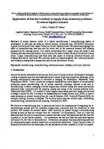
Behavior of the system for Tprz=1 is depicted in Figure 2. I np

I np D2

Qodz s

1

t2

2

t3

Q prod

Q prod

Q prod t1

Qodz

3

t4

4

t5

5

t6

6

t7

Qodz

7

t8

8

t9

9

t10

10

t11

11

t12

12

time

Iz Iz Qu su Qodz t1

1

t2

2

t3

3

t4

Qodz

Z4

4

Qodz t5

5

t6

6

t7

7

t8

8

t9

9

t10

10

t11

Figure 2. System behavior

105

11

t12

12

time

RT&A # 01 (24) (Vol.1) 2012, March

M. Plewa, A. Jodejko-Pietruczuk – THE REVERSE LOGISTICS FORECASTING MODEL WITH WHOLE PRODUCT RECOVERY

3.1

The method of forecasting the number of objects returned to the system

Presented model of reverse logistics system required to develop methods for forecasting the number of objects returned to the system, within a specified period of time, at a fixed time limit dop. Proposed forecasting model is a extension of model presented by Murayama in the (Murayama & Shu 2001, Murayama et al. 2004, 2005, 2006). The value of a dop depends on aging process and total costs. Therefore, whether the object at the time t is located in a recovery system depends on:  random variable Dzr,te specifying the number of objects placed on the operating system at the moment te,  random variable determining the probability of a technical object failure until dop. The probability of the object failure in the time interval from x1 to x2 can be written as follows (Migdalski 1982):

F  x1 , x2   P  x1    x2 

(12)

where  = random variable that describes the time to object failure. For tb-ta