Abstractâ Prior work motivated the use of sequential decoding for the problem of large-scale detection in sensor networks. In this paper we develop the metric ...
The sequential decoding metric for detection in sensor networks B. Narayanaswamy, Yaron Rachlin, Rohit Negi and Pradeep Khosla Department of ECE Carnegie Mellon University Pittsburgh, PA, 15213 Email: {bnarayan,rachlin,negi,pkk}@ece.cmu.edu
Abstract— Prior work motivated the use of sequential decoding for the problem of large-scale detection in sensor networks. In this paper we develop the metric for sequential decoding from first principles, different from the Fano metric which is conventionally used in sequential decoding. The difference in the metric arises due to the dependence between codewords, which is inherent in sensing problems. We analyze the behavior of this metric and show that it has the requisite properties for use in sequential decoding, i.e., the metric is, 1) expected to increase if decoding proceeds correctly, and 2) expected to decrease if more than a certain number of decoding errors are made. Through simulations, we show that the metric behaves according to theory and results in much higher accuracies than the Fano metric. We also show that due to an empirically-observed computational cutoff rate, we can perform accurate detection in large scale sensor networks, even when the optimal Viterbi decoding is not computationally feasible.
I. I NTRODUCTION The term “large scale detection” characterizes sensor network detection problems where the number of hypotheses is exponentially large. Examples of such applications include the use of seismic sensors to detect vehicles [5], the use of sonar to map a large room [6] and the use of thermal sensors for high resolution imaging [10]. In these applications the environment can be modeled as a discrete grid, and each sensor measurement is effected by a large number of grid blocks simultaneously (‘field of view’), sometimes by more than 100 grid blocks [10]. Conventionally, there have been two types of approaches to such problems. The first set of algorithms are computationally expensive such as Viterbi decoding and belief propagation [7]. These algorithms are at least exponential in the size of the field of view of the sensor, making them infeasible for many common sensing problems. The second set of algorithms make approximations (such as independence of sensor measurements [6]) to make the problem computationally feasible, at the cost of accuracy. Thus, there has existed a trade-off between computational complexity and accuracy of detection. Our previous work in [8] has defined the concept of ‘sensing capacity’ as the ratio of target positions to number of sensors, required to detect an environment to within a specified accuracy. Based on parallels between communication and sensing established by this work, [10] built on an analogy between sensor networks and convolutional codes, to apply a heuristic algorithm similar to the sequential decoding algorithm of convolutional codes, for the problem of detection in sensor networks. The average decoding effort of sequential decoding
is independent of the code memory, if the rate is below the computational cutoff rate of the channel. Therefore, by analogy, it is expected that the same independence applies to the problem of sensor network decoding, so long as enough measurements are collected (to keep the rate below the cutoff rate of the sensor network.) Such a computational cutoff rate behavior was indeed empirically observed in [10]. Thus, the paper demonstrated that the trade-off between computational complexity and detection accuracy can be altered by collecting additional sensor measurements. While [10] developed the possibility of using sequential decoding in sensor networks, the metric used there (the Fano metric) originated in the decoding of convolutional codes. The Fano metric is not justifiable for sensor networks, except perhaps in special cases. The main contribution of the present paper is the derivation of a sequential decoding metric for sensor networks from first principles, following arguments analogous to those used by Fano [3] for convolutional codes. The derived metric differs significantly from the Fano metric, due to the dependence between the ‘codewords’ that is inherent in sensor networks [8]. We analyze the behavior of this metric and show that it has the requisite properties for use with sequential decoding. i.e., the metric is expected to, 1) increase if decoding proceeds correctly, and 2) decrease if more than a certain number of decoding errors are made. In simulations, the metric behaves as predicted by theory and results in significantly lower error probability than the Fano metric. We also show that, due to an empirically-observed computational cutoff rate, we can perform accurate detection in large scale sensor networks, even in cases where the optimal Viterbi decoding is not computationally feasible due to the wide field of view of the sensors. II. S ENSOR N ETWORK M ODEL We consider the problem of detection in one-dimensional sensor networks. While a heuristic sequential decoding procedure has been applied to complex 2-D problems [10] using essentially the same model as the one described below, we present the 1-D case for ease of understanding and analysis. Motivated by parallels to communication theory and prior work, we model a contiguous sensor network as shown in Fig. 1. In this model, the environment is modeled as a kdimensional discrete vector v. Each position in the vector can represent any binary phenomenon such as presence or absence of a target. Possible target vectors are denoted by
derive an appropriate metric for sequential decoding in sensor networks. A. Definitions
Fig. 1.
Contiguous sensor network model
vi i ∈ 1, . . . , 2k . There are n sensors and each sensor is connected to (senses) c contiguous locations vt , . . . , vt+c−1 . The noiseless output of the sensor is a value x ∈ X that is an arbitrary function of target bits to which it is connected, x = Ψ(vt , . . . , vt+c−1 ). For example, this function could be a weighted sum, as in the case of thermal sensors, or location of the nearest target, as in the case of range sensors. The sensor output is then corrupted by noise according to an arbitrary p.m.f. PY |X (y|x) to obtain a vector of noisy observations y ∈ Y. We assume that the noise in each sensor is identical and independent so that observed sensor output vector isQrelated to the noiseless sensor outputs as n PY|X (y|x) = l=1 PY |X (yl |xl ). Using this output y, the decoder must detect which of the 2k target vectors actually occurred. Many applications also have a distortion constraint that the detected vector must be less than a distortion D ∈ [0, 1] from the true vector, i.e., if dH (vi , vj ) is the Hamming distance between two target vectors, the tolerable distortion region of vi is Dvi = {j : k1 dH (vi , vj ) < D}. Detection using this contiguous sensor model is hard because adjacent locations are often sensed together and have a joint effect on the sensors sensing them. III. S EQUENTIAL
DECODING FOR DETECTION
We adopt a sequential decoding procedure for inference, based on the stack algorithm described in [4]. This algorithm searches a binary tree consisting of all possible target hypotheses. In sequential decoding of convolutional codes, for a code of rate nk , each node in the tree corresponds to a set of n transmitted bits. There will be 2k branches leaving every node one for each possible assignment of values to the k input bits that generated the n transmitted bits. Similarly, in the case of sensor networks, each node in the tree corresponds to a group of sensors sensing the same set of locations, and each branch in tree corresponds to a hypothesis of the values of the locations sensed only by these sensors and not by any of the sensors previously decoded in the tree. Each of these hypothesis is evaluated using an appropriate metric and then inserted into a stack which holds all currently active hypothesis. This stack is then sorted according to metric values. All the branches extending from the topmost hypothesis in the stack (the hypothesis with the largest metric) are evaluated and the new hypotheses are inserted into the stack. This procedure is repeated until either a hypothesis of length equal to the target vector is obtained or some maximum number of steps is reached. The choice of metric is of primary importance in the design of sequential decoding algorithms. We now proceed to
In this paper we parallel the reasoning in [3], where a metric for sequential decoding was derived for decoding convolutional codes and extend that reasoning to the problem of detection in sensor networks. We use an argument similar to the random coding argument [11], that deals with the complications of inter-codeword dependence using arguments based on the method of types [1]. We first introduce the notation related to the types used and the random coding distributions. The rate R of a sensor network is defined as the ratio of number of target positions being sensed (k) to number of sensor measurements (n) R = nk . D(P ||Q) represents the Kullback-Leibler distance between two distributions P and Q. A sensor network is created as follows. Each sensor independently connects to c target locations according to the contiguous sensor network model as described in Section. II. When we consider all such randomly chosen sensor networks (similar to the random coding argument in communication theory), the ideal sensor outputs Xi associated with a particular target configuration Q vi is random. We can write this n probability as PXi (xi ) = l=1 PXi (xil ). A crucial fact is that the sensor outputs are not independent of each other, and are only independent given the true target configuration. The random vectors Xi and Xj corresponding to different target vectors vi and vj are not independent. Because of the sensor network connections to the target vector, similar target vectors (vs) are expected to result in similar sensor outputs (xs). We proceed to define the concepts of circular c-order types and circular c-order joint types [1] as they apply to our problem. A circular sequence is one where the last element of the sequence precedes the first element of the sequence. The circular c-order type γ of a binary target vector sequence vi is defined as 2c dimensional vector where each entry corresponds to the frequency of occurrence of one possible subsequences of length c. For example for a binary target vector and c = 2, γ = (γ00 , γ01 , γ10 , γ11 ), where γ01 is the fraction of subsequences of length 2 in vi which are 01. While all types are assumed circular we omit the word “circular” in the remainder of this section for brevity. Since each sensor selects the target positions it senses independently and uniformly across the target positions, PXi (xi ) depends only on the type Qnγ ofγ vi and can be written as γ,n PXi (xi ) = PX (x ) = i l=1 PXi (xil ) and is the same for i all vs of the same type γ. We define λ as the vector of λ(a)(b) , the fraction of positions vi has subsequence a and vj has subsequence b. For example when c = 2, λ = (λ(00)(00) , . . . , λ(11)(11) ), where λ(01)(11) is the fraction of subsequences of length 2 where vi has 01 and vj has 11. The joint probability PXi Xj (xi , xj ) depends only on the joint type of target vectors vi and vj and we can write PXi Xj (xi , xj ) = Qn λ,n PX (xi , xj ) = l=1 P λ (xil , xjl ). i Xj There are two important probability distributions that arise in the discussions to follow. The first is the joint
distribution between the ideal output xi when vi occurs, and its corresponding noise corrupted output y. This Qn is written as P (x , y) = P = X Y i X i Y (xil , yil ) i l=1 Qn (x )P (y |x ). The second distribution is the P il l il X Y |X i l=1 joint distribution between the ideal output xj corresponding to vj and the noise corrupted output y generated by the occurrence of xi corresponding to a different target vector vi . Qn (i) This is denoted as QXj Y (xj , y) = l=1 QiXj Y (xjl , yl ) = Qn P l=1 a∈X PXj Xi (xjl , xi = a)PY |X (yl |xi = a). Again the important fact should be noted that even though Y was produced by Xj , Y and Xi are dependent because of the dependence of Xi and Xj . We can reduce c-order type over a binary alphabet V to a 2-order type over a sequence with symbols in an alphabet V (c−1) of cardinality 22(c−1) by mapping each shifted binary subsequence of length c − 1 to a single symbol in this new alphabet. We ′ define λ = {λ(a)(b) , ∀a, b ∈ V (c−1) } as a probability P ′ ˜ mass function with λ(a)(b) = a,b∈V λ(aa),(bb) and λ = (c−1) {λ(a)(a)(b)(b) , ∀a, b ∈ V , ∀a, b ∈ V} as a conditional ˜ (aa)(bb) = λ(aa)(bb) . Correspondingly, we define γ ′ = with λ λ(a)(b) P ′ ′ {γa , ∀a ∈ V (c−1) } with γa = a∈V γaa and a conditional γ γ˜ = {γ˜aa , ∀a ∈ V (c−1) , ∀a ∈ V} defined as γ˜aa = (a)(a) γ(a) . B. Metric derivation
indexed by j. However, as described in Section. III-A these terms can be represented in terms of the type γ of xi and joint type λ of xi and xj . If we can tolerate errors up to a distortion D we should require the posterior probability of the correct codeword to be much greater than that of all other codewords that have a distortion greater than D. Let Sγ (D) be the set of all joint types corresponding to codewords of target vectors v at a distortion greater than D. n Y γ PX (xil )PY |X (yl |xil ) ≥ (3) i l=1
X
β(λ, k)
λ∈Sγ (D)
n X Y
λ (xjl , xi = a)PY |X (yl |xi = a) PX j Xi
l=1 a∈X
where β(λ, k) is the number of vectors vj having a given joint ′ ˜ ′ type λ with vi , bounded by β(λ, k) ≤ 2k[H(λ|λ )−H(γ˜j |γj )] [8]. Since vi and vj have the joint type λ their types are the corresponding marginals of λ(because of our definition of P types being circular) i.e., γ = c λ(a)(b) and γia = jb a∈0,1 P b∈0,1c λ(a)(b) .There are only a polynomial number of types c−1 2(c−1) C(k) = 22(c−1) k 2 (k + 1)2 [1][8], and the expression becomes n Y ′ ′ γ k[H(λ˜∗ |λ∗ )−H(γ˜∗ |γ ∗ )] PX (x )P (y |x ) − C(k)2 il l il Y |X i
While deriving the metric to be used for detection in l=1 n X Y sensor networks, significant changes need to be made from λ∗ (xjl , xi = a)PY |X (yl |xi = a) ≥ 0 (4) PX [3] because the “codeword” sequences X are not independent j Xi a∈X l=1 or identically distributed. The optimum decoding procedure ∗ would be the MAP (Maximum A Posteriori) procedure which for an appropriate choose of λ from the set of all λs and ∗ looks to find the noiseless sensor outputs X that maximizes where γ is the marginal type corresponding to the joint type ∗ the joint probability PXi Y . The MAP procedure for the 1- λ . Taking log2 () and applying a limiting argument as n → ∞, D contiguous sensor network case reduces to the Viterbi we obtain the general form of the metric (which is expected algorithm, which is computationally expensive. This is feasible to be positive when the probability of the correct codeword only for sensors with smaller field of view (c) since it requires dominates erroneous codewords) to be, n the evaluation of each element in a state space of size 2c−1 X log2 [P γ (xil )PY |X (yl |xil )] − (5) at each step with number of steps linear in the length of the target vector. The computation grows exponentially with c, l=1 n ∗ ′ ′ ∗ and so we must use sub-optimal procedures. These methods X log2 [P γ (xil )PYλ |X (yl |xil )] − k[H(λ˜∗ ||λ∗ ) − H(γ˜∗ |γ ∗ )] usually rely on the fact that if probability of error is sufficiently l=1 small, then the a posteriori most probable X is expected to be The choice of λ∗ is based on the properties desired of the much more probable than all the other code words. We try to metric and is discussed in Section. III-D. P This leads us to the select a condition under which we may expect the performance choice of appropriate metric as Sn = ni=1 ∆i , where ∆i is of an algorithm to be good. Suppose that given the received the increment in the metric as each sensor is decoded. sequence y there exists a Xi such X that γ (6) p(xi , y) ≥ p(xj , y) (1) ∆i = log2 [P (xil )PY |X (yl |xil )] − ′ ′ ∗ ∗ ∗ ∗ γ λ j6=i log2 [P (xil )PY |X (yl |xil )] − R[H(λ˜∗ ||λ ) − H(γ˜∗ |γ )] If the sensor networks were generated according to the random There are two requirements of a metric to be appropriate for scheme described in Section. II, then we can approximate the sequential decoding. The first is that the expected value of the left and right hand sides of (1) with their average value over a metric increase as the decoding of the target vector proceeds random ensemble of sensor network configurations and target down the correct branches of the binary hypothesis tree. The vectors, along the lines of the random coding argument [11] second is that the metric should decrease along any incorrect as applied to sensor networks X [8]. (i) path in the tree that is more than a distortion D from the true PXi Y (xi , y) ≥ QXj ,Y (xj , y) (2) target vector. We analyze the metric derived and prove that it j6=i The right hand side of (2) has an exponential number of terms satisfies these requirements for appropriate choices of rate R because of the exponential number of incorrect codewords and representative joint type λ∗ .
EX,Y ∆i = EX,Y log2 [P γ (x)P (y|x)] − EX,Y log2 [P
γ∗
(x)P
λ∗
(7) ∗′
∗′
(y|x)] − R[H(λ˜∗ ||λ ) − H(γ˜∗ |γ )]
Where expectation is over X and Y which are respectively, the noiseless and noise corrupted sensor outputs along the correct path. This reduces to (λ∗ )
= D(PXY ||QXi Y ) ′ ′ − R[H(λ˜∗ ||λ∗ ) − H(γ˜∗ |γ ∗ )]
EX,Y ∆i
(8)
which will be greater than or equal to 0 if we chose rate R such that (λ)
R≤
min
λ P λ ≥D Pa6=b ab b λab =γia
D(PXY ||QXi Y ) ˜ ′ ) − H(˜ [H(λ||λ γ |γ ′ )]
(9)
We note that the right hand side of (9) is expression for a lower bound on sensing capacity for a sensor network derived in [8]. Thus as long as the number of sensors used is sufficiently high so that the rate R is below the sensing capacity the metric will increase along the correct path.
50 0 −50 −100 −150
0
50
100
150
Sensors Decoded 300
Fano metric
We calculate the expected value of the increment in the metric ∆i along the correct decoding path and derive the condition on the sensor network for the expected value of these increments to be positive along this path.
New metric
C. Analysis of the metric along the correct path
200 100 0 −100 0
50
100
150
Sensors decoded
Fig. 2. Behavior of new metric and Fano metric along the correct path(in bold) and incorrect paths at a distortion D=0.02 away from the correct path for c = 15
The convexity of Sγ (D) can be reasoned as follows. The set of λ ∈ Sγ (D) are a group of probability mass functions defined by 1) a normalization constraint to ensure that they are true probability distributions 2) a set of markov constraints so that they are associated with real sequences and 3) a distortion constraint so that they correspond to sequences more than a distortion D from the true target vector. These constraints are preserved by a convex combination, implying that a convex combination of two valid λ ∈ Sγ (D) is a valid λ ∈ Sγ (D). Thus the set of λ ∈ Sγ (D) is convex and closed. Each probability distribution Qλ is linear in the elements of λ [8] and hence the set of Qλ is convex and the theorem can be applied.
D. Analysis of the metric along an incorrect path We now analyze the change in metric over an incorrect path corresponding to a vector vj having a joint type λ with the true target vector. We calculate the expected value of the increment in the metric ∆i along this path. EX ′ ,Y ∆i = EX ′ ,Y log2 P γ (x)P (y|x) − (10) ′ ′ ∗ ∗ EX ′ ,Y log2 P γ (x)P λ (y|x) − R[H(λ˜∗ ||λ∗ ) − H(γ˜∗ |γ ∗ )] ′
where X is the noiseless sensor outputs along the wrong path and Y is the noise corrupted true sensor outputs. EX ′ ,Y ∆i =
X
∗
Qλ (x, y) log2 (
X′ Y
P γ (x, y) ) Qλ∗ (x, y)
′
′
−R[H(λ˜∗ ||λ∗ ) − H(γ˜∗ |γ ∗ )] ∗
λ∗
≤ −D(Q ||P
γ∗
)− ≤0
′ R[H(λ˜∗ ||λ∗ )
(11)
∗
= −D(Qλ ||P γ ) + D(Qλ ||Qλ ) ′ ′ −R[H(λ˜∗ ||λ∗ ) − H(γ˜∗ |γ ∗ )] −
H(γ˜∗ |γ ∗
′
)]
(12) (13) (14)
Eqn. (13) is true if choose, ∗
λ∗ = arg min D(Qλ ||P γ ) λ∈Sγ (D)
(15)
Eqn. (13) arises from (12) because the set Sγ (D) is closed and convex, and using Theorem 12.6.1 in [2]. Eqn. (14) is from ′ the positivity of KL divergence [2] and since [H(λ˜∗ ||λ∗ ) − ′ ∗ H(γ˜∗ |γ )] > 0 since the γs are marginals of λs .
IV. S IMULATION R ESULTS Prior work [10] has compared sequential decoding with other algorithms such as belief propagation, occupancy grids and iterated conditional modes for a different sensing task. Since the inference task in this paper can be solved optimally by Viterbi decoding, we do not simulate these other approximate algorithms. We simulate a random sensor network at a specified rate R with sensors drawn randomly according to the contiguous sensor model. Error rates and runtimes for sequential decoding are averaged over at least 5000 runs. The output of each sensorP is the weighted sum of target regions in its field of view x = cj=1 wj vt+j . This output is discretized into one among 50 levels equally distributed between 0 and the maximum possible value and corrupted with exponentially distributed noise to obtain the discrete sensor outputs y. This has to be processed to detect the target vector. If the detected target v ˆ is more than a distortion D away from the true target vector an error occurs. An important part of the algorithm is the computation of λ∗ and the corresponding correction term. In this paper we assume that λ∗ is a joint type at a distortion D from the true vector and calculate the correction term for this λ∗ using a dynamic programming algorithm. In Fig. 2 we simulate the growth of the metric along the correct path and wrong paths at a distortion D from the true path. The behavior of the new metric is compared to that of the Fano metric where the increment is defined to be [3]: ∆Fi = log2 [PY |X (yl |xil )] − log2 PYl (yl ) − R
(16)
4
Running time of Viterbi decoding Running time of Sequential decoding
Running time in seconds
3
10
2
10
1
10
0
10
−1
10
−2
10
2
4
6
8
10
12
14
16
Sensor field of view c
Fig. 3. Comparison of running times of optimal Viterbi decoding and sequential decoding for different sensor fields of view c
Steps till convergence
Word error rate
10
0
10
−1
10
−2
10
1
0.9
0.8
0.7
0.6
0.5
0.4
0.3
0.2
0.5
0.4
0.3
0.2
Rate 2500 2000 1500 1000 500
1
0.9
0.8
0.7
0.6
Rate
Fig. 4. Running times and error rates for sequential decoding at different rates for c = 15 0
10
−1
10
Error Rate
Fig. 2 shows the important difference between the new metric and the Fano metric. Even when we proceed along an erroneous path that is at a distortion D away from the true path, the Fano metric continues to increase. This is because the Fano metric was derived assuming that if a path diverges from the true path at any point, the bits of the two codewords will be independent from that point onwards. While this is approximately true for strong convolutional codes with large memory, where the Fano metric has been used successfully, it is not a good assumption in sensor networks due to dependent distribution of codewords. Thus, if because of noise, the decoder starts along one of these erroneous paths, it could continue to explore it since the metric increases resulting in errors in decoding. When the new metric is used, the metric for the wrong path at distortion D decreases after the error, while the metric of the correct path is still increasing, verifying the properties previously derived. Thus we expect that the new metric would perform better than the Fano metric when used in a sequential decoder. The optimal decoding strategy in this sensor network application is Viterbi decoding. The computational complexity of Viterbi decoding increases exponentially in the size of the sensor field of view c. However the computational complexity of sequential decoding is seen to be largely independent of the sensor range c. This is illustrated in Fig. 3, which compares the average running times of sequential decoding and Viterbi decoding. While Viterbi decoding is not feasible for sensors with c > 8, sequential decoding can be used for much larger c values. Many real world sensors such as thermal sensors [10] or sonar sensors [6] have such large fields of view, demonstrating the need for sequential decoding algorithms. As with channel codes, sequential decoding has a higher error rate than optimal Viterbi decoding, and so is recommended only when Viterbi decoding is infeasible i.e., for large field of view sensors. The performance is reasonable given the low computation time even when Viterbi is too complex to be feasible. The primary property of sequential decoding is the existence of a computational cutoff rate. In communication theory, the computational cutoff rate is the rate below which average decoding time of sequential decoding is bounded. The complexity of Viterbi decoding on the other hand, is almost independent of the rate. We demonstrate through simulations that a computational cutoff phenomenon exists for detection
−2
10
Word error rate with new metric Word error rate with Fano metric
−3
10
Bit error rate with new metric Bit error rate with Fano metric 0
0.01
0.02
0.03
0.04
0.05
0.06
0.07
0.08
0.09
0.1
Distortion
Fig. 5. Comparison of error rates of new metric and Fano metric for different tolerable distortions at rate 0.2 for c = 15
in large scale sensing problems using the new metric. The results of these simulations are shown in Fig. 4. This leads us to an alternative to the conventional trade-off between computational complexity and accuracy of detection, where this trade-off can be altered by collecting additional sensor measurements, leading to algorithms that are both accurate and computationally efficient. Finally we compare the performance of sequential decoding when the new metric is used and when the Fano metric is used as a function of the tolerable distortion in Fig. 5. The Fano metric does not account for the distortion in any way and we can see that its performance is much worse. R EFERENCES [1] Imre Csiszar, “The Method of Types,” in IEEE Trans. on Info. Theory, Vol:44, 2502-2523, 1998. [2] Thomas M. Cover and Joy A. Thomas, “Elements of Information Theory,” John Wiley and Sons, Inc., New York, N.Y., 1991. [3] R. Fano, “A heuristic discussion of probabilistic decoding,” in IEEE Trans. on Info. Theory,Vol 9:2, 64-74, Apr 1963 [4] F. Jelinek, “A fast sequential decoding algorithm using a stack,” in IBMJ. Res. Dev., 13, 675685, 1969. [5] D. Li, K. Wong, Y. Hu, and A. Sayeed, “Detection, classification and tracking of targets in distributed sensor networks,” in IEEE Signal Processing Magazine, 1729, March 2002. [6] H. Moravec and A. Elfes, “High resolution maps from wide angle sonar,” in IEEE International Conference on Robotics & Automation, 1985. [7] J. Pearl, “Probabilistic Reasoning in Intelligent Systems: Networks of Plausible Inference,” Morgan Kaufmann, 1988. [8] Y. Rachlin, R. Negi, and P. Khosla, “The Sensing capacity of Sensor Networks,” submitted to IEEE Trans. on Info. Theory, www.ece.cmu.edu/˜rachlin/pubs/SensingCapacity Submission.pdf [9] Y. Rachlin, R. Negi, and P. Khosla, “Sensing capacity for discrete sensor network applications,” in IPSN05, Apr 25-27 2005. [10] Y. Rachlin, B. Narayanaswamy, R. Negi, John Dolan, and P. Khosla, “Increasing Sensor Measurements to Reduce Detection Complexity in Large-Scale Detection Applications,” in Proc. MILCOM06, 2006. [11] C. E. Shannon, “A mathematical theory of communication,” Bell Syst. Tech. J., vol. 27, pt. I, pp. 379–423, 1948; pt. II, pp. 623–656, 1948.