Molecular Ecology Resources (2012) 12, 1058–1067
doi: 10.1111/1755-0998.12003
The simple fool’s guide to population genomics via RNA-Seq: an introduction to high-throughput sequencing data analysis PIERRE DE WIT,* 1 MELISSA H. PESPENI,*† 1 JASON T. LADNER,* DANIEL J. BARSHIS,* FRANC ¸ OIS SENECA,* HANNAH JARIS,* NINA OVERGAARD THERKILDSEN,‡ MEGAN MORIKAWA§ and STEPHEN R. PALUMBI* *Department of Biology, Stanford University, Hopkins Marine Station, 120 Ocean view Blvd., Pacific Grove, CA 93950, USA, †Department of Biology, Indiana University, 915 E. Third Street, Myers Hall 150, Bloomington, IN 47405-7107, USA, ‡National Institute of Aquatic Resources, Technical University of Denmark, Vejlsøvej 39, 8600, Silkeborg, Denmark, §Duke University, Durham, NC 27708, USA
Abstract High-throughput sequencing technologies are currently revolutionizing the field of biology and medicine, yet bioinformatic challenges in analysing very large data sets have slowed the adoption of these technologies by the community of population biologists. We introduce the ‘Simple Fool’s Guide to Population Genomics via RNA-seq’ (SFG), a document intended to serve as an easy-to-follow protocol, walking a user through one example of highthroughput sequencing data analysis of nonmodel organisms. It is by no means an exhaustive protocol, but rather serves as an introduction to the bioinformatic methods used in population genomics, enabling a user to gain familiarity with basic analysis steps. The SFG consists of two parts. This document summarizes the steps needed and lays out the basic themes for each and a simple approach to follow. The second document is the full SFG, publicly available at http://sfg.stanford.edu, that includes detailed protocols for data processing and analysis, along with a repository of custom-made scripts and sample files. Steps included in the SFG range from tissue collection to de novo assembly, BLAST annotation, alignment, gene expression, functional enrichment, SNP detection, principal components and FST outlier analyses. Although the technical aspects of population genomics are changing very quickly, our hope is that this document will help population biologists with little to no background in high-throughput sequencing and bioinformatics to more quickly adopt these new techniques. Keywords: bioinformatics, de novo assembly, gene expression, population genomics, RNA-Seq, SNP detection Received 13 March 2012; revision received 16 July 2012; accepted 27 July 2012
Introduction High-throughput sequencing technologies are today capable of sequencing billions of bases in a single sequencing reaction (Hudson 2008; Morozova et al. 2009). These revolutionary techniques allow researchers to sequence entire genomes or transcriptomes (Wang et al. 2009) on a population-wide scale at reasonable cost and are currently revolutionizing our view of many important biological concepts, such as natural selection (Pickrell et al. 2009; Yi et al. 2010; Pespeni et al. 2011), gene flow (Tishkoff et al. 2009; Neafsey et al. 2010) and gene expression patterns (Wolf et al. 2010; Renaut & Correspondence: Pierre De Wit, Fax: (831) 375-0793; Email:
[email protected] 1
Equally contributing authors.
Bernatchez 2011). For example, Price et al. (2012) recently used high-throughput sequencing to simultaneously assemble nuclear, mitochondrial and chloroplast genomes of the basal alga Cyanophora paradoxa and to unambiguously demonstrate a single origin of all algal and plant chloroplasts in the face of a complex pattern of reticulate evolution. Barakat et al. (2009) used 454 sequencing to assemble Chestnut transcriptomes to find genes and functional pathways involved in resistance to a parasitic fungal infection, opening the door for genetic engineering of resistant trees (Barakat et al. 2009). Similarly, Poelchau et al. (2011) assembled a transcriptome of an invasive disease-carrying mosquito and identified genes involved in diapause, which allows mosquitos to survive harsh winters, research that might lead to better control of mosquito-transmitted diseases in the future.
© 2012 Blackwell Publishing Ltd
S I M P L E F O O L ’ S G U I D E T O P O P U L A T I O N G E N O M I C S 1059 Yet, the computational power and bioinformatics knowledge needed to process and successfully analyse these immense data sets have slowed adoption of this approach for a large number of population biologists. Increasingly powerful desktop computers make it possible to analyse short-read DNA sequence data, but analytical approaches are still being developed (e.g. Grabherr et al. 2011; Haridas et al. 2011; Mizrachi et al. 2011), and new software is being written constantly (Li & Durbin 2009; Simpson et al. 2009; Boisvert et al. 2010; Martin et al. 2010; Pitt et al. 2010; DePristo et al. 2011). Increasingly, published studies tend to omit many of the steps needed to move from tissue sample to analysis. Consequently, a great deal of trial and error is demanded in every new laboratory taking up these tools. Further, most analysis software to date require considerable knowledge of computer scripting and micro-programming. In many cases, there is a demand for custom-made scripts to move from one analysis step to another, but how to write or execute these requires learning a new skill set (See Haddock & Dunn (2011)). Thus, there is a need for an easy-to-follow guide that walks the user through the steps needed from tissue collection, to acquiring gene expression and genotype data on genome or transcriptome-wide scales, to data analysis and visualization. In this article, we introduce the ‘Simple Fool’s Guide to Population Genomics via RNA-Seq’ (from here on ‘SFG’), available at http://sfg.stanford.edu, a tool intended as a guide to help researchers dealing with nonmodel organisms start to acquire and process highthroughput sequencing data. It aims at walking population biologists with little to no background knowledge in computer programming through an example analysis of high-throughput sequencing data. It is intended as an example of one way to process this kind of data, to address a few specific biological questions (outlined below). By getting started with a simplified analysis for which scripts are already written, our intention is to lower the steepness of the initial learning curve. After walking through this protocol and focusing on bioinformatic methods, the user will have acquired many skills that will be useful for creating their own custom analysis. In the long run, users will likely want to learn how to write their own scripts in Perl or Python, a topic that is not included in this protocol. However, by studying how the scripts within this protocol are structured in combination with more general bioinformatic learning material such as Haddock and Dunn’s ‘Practical Computing for Biologists’ (2011), the user will be at an optimal starting point for further learning. We recognize that any SFG to Population Genomics is partially obsolete already when published owing to the speed with which the field is developing; but our aim is
© 2012 Blackwell Publishing Ltd
to get the reader started, leaving future developments to be incorporated as needed. The SFG covers tissue collection, library preparation and computer setup and includes data quality control, transcriptome assembly and extraction of SNP and gene expression data.
High-throughput sequencing in population biology There are numerous techniques currently in use that are associated with high-throughput sequencing. Population-wide whole-genome shotgun sequencing (Weber & Myers 1997) data are still technically difficult to analyse in nonmodel organisms, as repeat regions and insertions and deletions in noncoding regions complicate assembly. Also, an intense sequencing effort is required to gain sufficient sequencing depth throughout unknown genomes to confidently identify variant sites. This issue is now starting to become less problematic with the extremely high output and lower cost of new sequencing machines. Also, development of new inferential methods for assignment of genotypes from pooled individuals is likely to decrease the coverage needed in the future (Li 2011). Yet, these issues must still be kept in mind when choosing the sequencing technique for a new project. An option is to initially sequence the genome of one individual through BAC library Sanger sequencing and then resequence more individuals using a high-throughput platform, as was recently performed by Jones et al. (2012). This approach was successful in locating adaptive sequences throughout the genome. However, the initial genome sequencing was both time-consuming and costly. In addition, current population-based genome resequencing studies often rely on experimentally inbred lineages (e.g. in Drosophila (Andolfatto et al. 2011; Turner et al. 2011)), which is not feasible for studying variation in natural populations. As a result, it seems as if practical access to genomewide information from nonmodel organisms currently requires that the entire genome be reduced in some way. One way to do this is to concentrate on regions that surround predefined restriction sites, used in the Genotypingby-Sequencing (Elshire et al. 2011), CRoPS (van Orsouw et al. 2007) and RAD-Tag sequencing (Hohenlohe et al. 2010) techniques. These methods provide a cost-effective way of identifying variant sites throughout the genome (Davey et al. 2011), because many individuals can be combined in one sequencing run by using barcoded adapters, while still maintaining a high coverage over the reduced representation library. These techniques have successfully been used for genome-wide association studies in species with high chromosomal linkage, such as the Diamondback moth and Barley (Baxter et al. 2011; Chutimanitsakun et al. 2011), and are very useful for studying phenomena such as introgression and
1060 P . D E W I T E T A L . genome-wide population differentiation with a high number of loci. Because data from these approaches are scattered at sites across the genome, they usually occur in nongenic regions, which do not provide any information on the function of the variant-containing sequence unless annotated genomic sequence information also is available or the sites in question are tightly linked to particular genes. Another genome-reducing framework is RNA-Seq (Wang et al. 2009), in which the focus is on sequencing only mRNA from the genes that are expressed in a tissue (the ‘transcriptome’), wherein a significant proportion of adaptively interesting variation is located. Jones et al. (2012), for example, found that up to 60% of putatively adaptive sites in sticklebacks were located in proteincoding positions, the rest being located in regulatory regions. The great advantage of RNA-Seq is that functional information for sequences can be obtained by comparing to known genes in other organisms, side-stepping the need for pre-existing species-specific genomic information. Also, this method provides gene expression data in addition to variant DNA bases, as it is possible to compare counts of reads that map to any given gene between individuals. An important issue when working with RNA, however, is RNA instability; mRNA degrades very quickly, so it is very important to promptly process tissue samples in buffer solutions and at low temperatures to avoid degradation.
Purpose and scope of the SFG In the SFG, we focus on RNA-Seq data, although the approach we outline also is useful for other highthroughput sequencing methods. This is by no means an exhaustive protocol, and there are many other ways to process and analyse high-throughput sequencing data. However, the methods outlined herein provide an approachable, functional starting platform with which to build the bioinformatic skills required to subsequently create a custom analysis protocol. The protocol can be used for organisms for which there are no current genomic resources, or for those with fully sequenced and annotated genomes or transcriptomes, in which case some steps can be omitted. All instructions are written for Mac OS X, but will also work (with slight modifications) on a machine running Linux or in Windows through a UNIX/Linux portal. The SFG is divided into eight sections. An initial section on sample preparation is followed by a guide on how to set up a Macintosh computer properly, after which there are six major sections on data processing (Fig. 1). Within the data processing pipeline, if there are genomic resources available for the study organism, the de novo assembly and annotation sections can be omitted.
Sections on quality control processing, de novo assembly, BLAST comparison and mapping to reference are data processing steps, whereas the gene expression and SNP detection and analysis sections start addressing biological questions. For each section, we provide a narrative guide with some of the intrinsic trade-offs of different approaches. Most of the technical details – from specific laboratory protocols to scripts to statistical approaches – change rapidly enough that we provide them as an online resource available at http://sfg. stanford.edu.
Tissue collection and sample preparation Basic themes Depending on the goal of the project and resources available for the study organism, the user will want to prepare samples in accordance with the sequencing technique that provides the most information. Wholegenome sequencing can provide information on sequence variation throughout the entire genome. However, this approach works best if there already is a conspecific genomic resource available. To create and annotate a de novo assembly of a genome is still a daunting task; it requires long reads (preferably from 454 sequencing), high coverage and time to discover genes and annotate them. By combining reads from different sequencing technologies, some of these issues can be dealt with (Nowrousian et al. 2010). Restriction enzyme– based approaches, such as Genotyping-by-Sequencing (GBS), can also provide genome-wide sequence variant information, without the need for a reference genome. GBS does not, however, provide any information on whether the variation detected is located in genes or not. Transcriptome sequencing (RNA-Seq) only provides information for expressed genes, but it gives two kinds of information: it is a record of how many mRNAs from a particular exon are in the sample, and it includes variants in the sequence that tell us about polymorphisms in the DNA. This is currently the only method for acquiring gene expression data in addition to sequence variation in genes, although issues such as sequencing error and amplification bias always need to be kept in mind when dealing with high-throughput sequencing data. There is a major difference in collecting strategies for these different empirical approaches. As genes are expressed differently in different tissues and times, mRNAs extracted from different parts of the same species will not be identical. Thus, an important first consideration is tissue sampling – the user needs to be consistent in tissue type and processing. The genes not expressed in these tissues will be invisible to the analysis, so think about what tissues would be optimal.
© 2012 Blackwell Publishing Ltd
S I M P L E F O O L ’ S G U I D E T O P O P U L A T I O N G E N O M I C S 1061
Gene expression analysis
Sequencing
Tissue collection Library preparation
Computer setup
Quality control processing of raw data
De novo assembly
BLAST
Mapping reads to a reference
SNP detection
Fig. 1 Workflow of the Simple Fool’s Guide to Population Genomics via RNA-Seq: Gene expression and SNP data analysis in the age of high-throughput sequencing.
Individuals sampled from the wild have had a different environmental and evolutionary history, so they are not expected to have identical expression patterns. Also, the user may be working in a system where gene expression is highly circadian, so sample timing is also important to consider. In most cases, it is the variation between individuals within a group compared with the variation between groups that will be the heart of a SNP or expression analysis, so choose sampling scheme carefully to reduce gene expression variance within groups or to maximize the chances of finding rare/local variants in a SNP analysis.
Approach Whole-genome or GBS library creation begins with highmolecular-weight DNA and generates a genome library by shearing the genomic DNA into an optimal size range or using restriction enzymes to cut the genomic DNA at certain sites that will be the starting point of all reads. RNA-Seq begins with extraction of RNA from fresh, frozen (at 80 °C) or preserved [in RNAlater (Qiagen, Valencia, CA, USA) or Trizol (Invitrogen, Grand Island, NY, USA)] tissue samples. This demands a series of extra steps including purification of mRNA from total RNA, fragmentation and synthesis of complementary DNA (cDNA) from the mRNA. Unlike DNA, RNA is highly labile: RNAlater makes it possible to preserve tissues in field settings. It is also quite easy to make a buffer solution acting like RNAlater (recipe available at http://sfg.stanford.edu). RNAlater works by quickly diffusing into cells, stabilizing mRNA and inactivating RNA-degrading RNases. It cannot diffuse into frozen tissue, so samples should be stored in RNAlater at refrigerator temperatures for a day or so before freezing. RNAlater samples can be kept at room
© 2012 Blackwell Publishing Ltd
temperature, but they decay at a slow rate. In our protocol, we use Qiagen’s ‘RNeasy’ RNA extraction kit (Qiagen) to extract total RNA from tissue, after which we use Illumina’s ‘TruSeq RNA Sample Prep Kit’ (Illumina, San Diego, CA, USA) to create cDNA libraries. The full SFG has more information, although the kits’ protocol worksheets are extensive and (eventually) self-explanatory. The cDNA libraries are then quality-assayed (generally using an Agilent Bioanalyzer or quantitative PCR) and sent to a sequencing centre for sequencing. No matter where the library DNA comes from (e.g. from sheared DNA, from restriction digested DNA, or from cDNA preparations), library constructions is similar. Tags (‘barcodes’) are placed on the ends of DNA molecules from each library, allowing each sample to be identified after sequencing. This means that several samples can be mixed into one sequencing run, thereby decreasing cost. There are many different tags available; for RNA-Seq, it is currently possible to multiplex 24 individuals in one run – although whether this renders enough data for each individual depends on the question being asked and the analytical power needed. The GBS protocol of Elshire et al. (2011) allows for a nearly unlimited set of individual DNA labels. Once the DNA libraries are created and amplified, they are ready to be sequenced, and it is time for a decision: what kind of sequencing platform would be most relevant? As of this writing, Illumina sequencing is most commonly performed in one of two ways: single-end 50 base pair reads or paired end 100 base pair reads. The latter tends to cost about twice the former, although four times more data are returned. Assemblies of transcriptomes of new organisms tend to be easier with paired end 100 bp reads. But if a reference transcriptome already exists, shorter reads might be adequate for mapping and analysing gene expression patterns or genotyping. Every
1062 P . D E W I T E T A L . project is unique, and the data type should be chosen with the project goal in mind.
Computer setup Basic themes The promise of high-throughput sequencing is a flood of data. Taking the time to set up the files and programs on a computer, so that it is possible to move step by step through the large number of different protocols is an efficient way to build the virtual laboratory bench needed. The SFG walks the user through the installation process on a Macintosh with an Intel processor and the Lion (OS X version 10.7) or Snow Leopard (OS X version 10.6) operating system. This does not mean that a Mac is required, but Mac OS X is currently one of the most commonly used operating systems for bioinformatics, along with various versions of the Linux operating system family. Properly setting up the computer is a challenge and will take at least a full day. Yet, the rewards are great in that the user will not have to stop constantly to troubleshoot cryptic error messages or install new software during data analysis steps. However, even with a properly configured computer, some tasks will take a long time or even be infeasible on a standard desktop computer. For most tasks, we recommend purchasing a new computer with as many processor cores as possible and the maximum possible RAM memory. For the most intensive tasks, such as de novo assembly (depending on software used) and gene annotation, access to computer clusters or online cloud services will be highly beneficial; many universities offer this type of services, so it might be worthwhile for the user to investigate what options are available.
Approach The protocol includes more than ten different software packages, using different file formats, programming languages and command line arguments, so making sure that the computer understands these is crucial before starting the data analysis. Detailed information on how to install software and set up a computer is given in the online version of the SFG. We propose creating one folder for scripts and one for programs in the home directory, where all software can be located, as well as one folder for data files (sub-folders optional). Modifying output files from one program into input files from the next or conducting statistical analyses on large amounts of data can also be a major hurdle. For this purpose, we also distribute a package of scripts along with the SFG, which can be found at http://sfg.stanford.edu. The scripts provided in the repository are free software with no warranty of any kind: they can by redis-
tributed and/or modified under the terms of the GNU General Public License (Free Software Foundation, version 3 of the License). A list of all software mentioned in the SFG, along with information on where to find it, can be found in table 1 of the SFG (see http://sfg.stanford. edu/software.html).
Quality control processing of high-throughput sequencing data Basic themes The day has arrived when the sequencing centre returns an immense number of short DNA sequences, ‘reads’, from the libraries submitted. Ideally, these would all be of perfect quality and represent the full diversity of mRNA (or genomic DNA, depending on method used) in a tissue. Yet, to make sure that this is the case, we need to scan through the huge data files using specialized software. We are looking for reads that are too short, reads with poor-quality base pair calls and artefacts from the sample preparation procedure.
Approach This section guides the user through the process of initial data processing of short reads generated with highthroughput sequencing. The first objective is to remove any adapter sequences (the tags put onto the DNA during sample preparation) and to perform a few simple quality control steps, such as graphing the distributions of quality scores (e.g. confidence levels for the DNA sequences) and calculating the fractions of duplicate and singleton reads in the data. A duplicate read is one that is identical to another in the data set. These should be rare, yet poor initial sample quality or bias during the final PCR step can elevate the numbers significantly (Note that GBS data can be expected to contain a higher fraction of duplicates). To perform these tasks, the software package ‘fastx toolkit’ (http://hannonlab.cshl.edu/fastx_toolkit/) is used in combination with provided scripts. Graphing is conducted on the Galaxy Web server (http://main.g2.bx. psu.edu/). At the end of this process, the user will have a list of high-quality DNA reads that will form the basis for the rest of the analysis.
De novo assembly Basic themes When dealing with nonmodel organisms, the lack of published genomes or transcriptomes onto which the reads can be mapped can be a major hurdle. Depending
© 2012 Blackwell Publishing Ltd
S I M P L E F O O L ’ S G U I D E T O P O P U L A T I O N G E N O M I C S 1063 on what species the user is working with, an EST library might be available on NCBI’s database. However, even these lists do not generally encompass all the expressed material in the new data. The next step is called ‘assembly’, and it searches for overlap among short reads and thereby builds longer and longer ‘contigs’. With restriction site–directed libraries, all reads start at a set of a few thousand up to millions of restriction sites. As a result, the ‘contigs’ will be aggregations of reads near those sites, no longer than the read length. For other approaches, the libraries are derived from randomly sheared DNA and so reads start at different places. This variability allows these reads to be joined together into contigs. De novo assemblies are tricky to create – ideally only reads from the same genes should line up, but there are many duplicate genes in some genomes and reads can get switched. In addition, whole gene sequences are seldom generated this way – except for very highly expressed genes, there are often several contigs per gene. Longer reads (say 100 bases vs. 50) produce better assemblies because the overlap can be better. Paired end reads (where sequences are read from both ends of a cDNA molecule) are also helpful. Lastly, the cDNA library includes sequences from more than the study organism. Bacterial and viral reads can be very common: there might also be gut content sequences present if gut tissues have been sampled. As a result, some contigs are not from the intended species. The basic idea in de novo assemblies is to use as much data as possible in creating contigs that represent genes in the species of interest and to take the results cautiously.
Approach The objective of this section is to use the graphical user interface application ‘CLC genomics workbench’ (http://www.clcbio.com/index.php?id=1240) (CLC bio, Cambridge, MA) to combine reads from all sequenced individuals into a de novo assembly. The assembly will be used as a reference transcriptome in the following sections. If a transcriptomic resource is available, this step can be omitted. There are many other approaches available (see e.g. Martin & Wang 2011; Baker 2012; Scally et al. 2012), but the CLC algorithm is less memory-intensive than most others and is currently the only practical option for desktop computers. Unless the transcriptome assembly is a major part of the research program, remember that the assembly is largely a means to an end, and it will not be perfect no matter what software is being used. The key aspect of the transcriptome is not that it is comprehensive, but that the contigs in it represent valid and unique sections of genes from the genome of interest.
© 2012 Blackwell Publishing Ltd
BLAST comparison to known sequence databases and functional annotation
Basic themes One of the major advantages of transcriptome sequencing is that the data come from functional, expressed genes. But this value will be minimal unless it is possible to identify these genes. The same is true of wholegenome assemblies, where some of the contigs are from exons within genes. One way to identify contigs is to compare each contig sequence with known genes and assume that homology tells something about function. Doing this for one or a few genes is easy using the BLAST search algorithm on the NCBI Web page – but with 10 000s or 100 000s of contigs, an automated approach is necessary. Also, BLAST searches against large databases take a long time (a BLASTx against NCBI’s nr database typically takes around 1 min per contig, so with 100 000 contigs, the search will take 70 days), so access to a computer cluster or a cloud service will be essential for this step. This way, the list of contigs can be split into many small files, BLAST searches can be run in parallel, and the run duration can be reduced to hours.
Approach Establishing links between observed sequence variation and gene function is a major challenge when analysing transcriptome data from nonmodel organisms (Pop & Salzberg 2008; Yandell & Ence 2012). Here, we describe a pipeline using the Basic Local Alignment Search Tool (BLAST; http://blast.ncbi.nlm.nih.gov/) to compare de novo assembled contigs to sequence databases to annotate them with similarity to known genes/proteins/ functions. Usually, the best way to look for homology is not at the nucleotide level, but rather at the protein level. By querying three major databases, GenBank’s nonredundant protein database (NR) and Uniprot’s Swiss-Prot and TrEMBL protein databases, we can identify the most similar known proteins for the translation of each contig. In addition to the gene name, there is a wealth of information in code form about the metabolic functions of many genes. To access these codes, we also describe a method to extract gene names, general descriptions and Gene Ontology (GO) categories (http://www.geneontology. org/) for significant BLAST matches. GO categories are alphanumeric codes that correspond with the metabolic roles known for a gene. These codes can be used in subsequent enrichment analyses for gene expression or SNP data. Finally, because all these data sets are complex, we provide a simple, single-reference data framework that
1064 P . D E W I T E T A L . houses all the de novo assembly annotation information for easy access by the user.
Mapping reads to a set of reference sequences Basic themes Mapping refers to the process of aligning short reads to a reference sequence, whether the reference is a complete genome, transcriptome or a de novo assembly. Reads are compared with the whole length of every contig in the assembly and the position where they match the best is noted. Does the match have to be perfect? No, and the criteria for calling something a match is something that needs to be adjusted. If a read matches more than one place, it must be discarded, as there is no way to figure out where the correct location is. Thus, it is important to choose mapping parameters to maximize the fraction of reads that match one place in the reference, yet minimize the fraction of reads that map to more than one place.
Approach There are numerous programs that have been developed to map reads to a reference sequence that vary in their algorithms and therefore speed (see Flicek & Birney 2009 and references therein). The program that we utilize in this pipeline is called BWA (Li & Durbin 2009). It uses a Burrow’s Wheeler Transform method that results in much faster processing than the first wave of programs that used a hash-based algorithm such as MAQ (Li et al. 2008). The sequence alignment files created in this step are also used in subsequent steps to extract expression information (the number of reads that map to each gene) and to identify polymorphisms across a data set. To obtain the highest number of high-quality mapped reads, it is important to optimize the alignment parameters for each study organism. For example, the number of differences between reference and query sequences is expected to vary with the polymorphism and recombination rates specific to a species.
Gene expression analysis from RNA-Seq data Basic themes Gene expression analysis from RNA-Seq data starts with extracting the number of reads that map uniquely to each contig or gene from alignment files. These count data will serve as a proxy for the magnitude of gene expression because transcripts of greater abundance in the cell will have more reads generated from libraries prepared from RNA. Gene expression may vary between samples or individuals in a study owing to experimental
design, for example control vs. treatment, or among ecotypes or morphs, time of sampling, tissue or origin. Once obtained, the density of data is likely to be different among individuals because of initial differences in RNA yield or library density. To compare among individuals, then, the data need to be bioinformatically ‘normalized’ (Oshlack et al. 2010) to account for differences in sequencing depth (note that this is different from normalizing cDNA libraries prior to sequencing). The simplest way would be to calculate the fraction of reads mapping to a contig out of the total number of reads. More complex procedures have been developed, but they have similar goals, making it possible to compare data sets.
Approaches The main objectives of this section are to (i) extract gene expression data for the sequence alignment files generated in the mapping step, (ii) detect differential gene expression among treatments, and (iii) identify transcriptome-wide patterns of enrichment for functional classes of proteins. Although it is not included in the SFG, RNASeq data can also be used to explore alternative splicing and allele-specific expression. This is a fairly detailed section, divided up into the three sub-sections above. Extracting read numbers per gene is straightforward – the reads associated with each contig are counted up. However, there are several important nuances to the data. In particular, different individuals in the data set will have different numbers of reads just because of chance or differences in mRNA, cDNA or library quality. To adjust for this, data for each sample need to be normalized against one another. A simple way to accomplish this is to estimate the number of reads per million mapped (Wang et al. 2009). Other, more sophisticated procedures normalize across samples for a particular contig, taking into account whether a particular individual tends to have lower or higher counts among all contigs than others (Oshlack et al. 2010; Robinson & Oshlack 2010). We begin with a popular software package, DESeq (Anders 2010). However, there are many other ways to operate, including producing a large spreadsheet of expression levels, arranged with contigs in different rows and individuals in different columns, principal components, statistical functions in R such as ANOVA or any other method that can deal with large data sets. The rule here is that the data are generally messy and that variation from individual to individual is common. The answers tend to be based on whether there is more variation between groups (say between experimental treatments) rather than within them. The other key feature of the analysis is that there are many statistical tests
© 2012 Blackwell Publishing Ltd
S I M P L E F O O L ’ S G U I D E T O P O P U L A T I O N G E N O M I C S 1065 involved; thus, corrections for multiple tests are critical. A P-value of 0.05 means nothing when differential selection is being tested for in 20 000 genes: one would expect 1000 to be different purely by chance. Benjamini– Hochberg correction, false discovery rate corrections and q-value calculation are common methods employed with genomic data to correct for multiple tests (Benjamini & Hochberg 1995; Storey & Tibshirani 2003). Last, it is important to realize that the gene (or contig) is not the only unit of analysis and that it is possible that entire metabolic pathways are differentially expressed without a single gene in the pathway being significant (often because of among-individual variation and multiple test corrections, see above). In this analysis, we group genes by function and ask whether the groups of genes differ in expression between individuals. There are several common sources of gene groups: UniProt, Gene Ontology, PANTHER and KeGG (Ogata et al. 1999; Ashburner et al. 2000; Thomas et al. 2003; Bairoch et al. 2009). Keep in mind that the gene functions coded in the above lists are generally the functions of that gene in mammals: their function in the study organism may be different. It is also possible to make up a list for metabolic functions under particular interest, such as biomineralization; these genes could be well characterized in the study organism. The nested nature and seeming redundancy of functional categories can make interpreting functional enrichment results a challenge. For example, the single transcription factor NF-kappaB may belong to 20 functional categories related to transcriptional regulation, inflammatory response, apoptosis and so on, all significantly enriched in the data. There are several tools that have been developed to simplify, visualize and help interpret functional enrichment results. Some useful programs include REViGO (Supek et al. 2011), Ontologizer (Bauer et al. 2008) and model-based gene set analysis [MGSA (Bauer et al. 2010)]. The GO website maintains an extensive list of programs (http://www.geneontology. org/GO.tools.microarray.shtml).
SNP detection and analysis Basic themes Single nucleotide polymorphisms (SNPs) are one of the fundamental types of genetic variation, and with the growing popularity of next-generation sequencing, they are becoming the most ubiquitously utilized genetic markers in analyses of both model and nonmodel organisms (Kim & Misra 2007; Dereeper et al. 2011; Geraldes et al. 2011; Helyar et al. 2011). Recall that when reads were mapped to the contigs, they did not have to be 100% perfect matches. When a read is mismatched to a contig at a single base, this is either a mistake or a
© 2012 Blackwell Publishing Ltd
polymorphism. When several reads include the mismatch (ideally, about half), then this individual may be a heterozygote for that single nucleotide polymorphism. By looking at all the base calls at all the polymorphic sites at all the reads in the data set, we can estimate the genotype of an individual at all these SNPs. This tends to be a huge number for a decently covered genome or transcriptome and represents a repository of much information about genetic structure and adaptation. The algorithms that detect SNPs and assign genotypes also take uncertainty (because of sequencing/PCR/alignment errors) into account and assign quality scores to each individual SNP and genotype, making it possible to filter out and ignore SNP sites or genotypes that fall below a quality threshold. In addition, maximum-likelihood and Bayesian models have been developed for improving the accuracy of detecting allele frequencies from next-generation sequencing data for population genomic analyses (Lynch 2009; Gompert & Buerkle 2011). A major challenge for the user is thus to find an optimal balance between quantity and quality of data.
Approaches Short reads from a single lane of an Illumina sequencer can easily result in the identification and genotyping of 10 000s of SNPs. An issue, however, is to separate true polymorphisms from sequencing or alignment artefacts (DePristo et al. 2011). The main objective of this section is to provide a step-by-step pipeline through thirdparty software packages [SAMtools (http://samtools. sourceforge.net/) (Li et al. 2009), Picard (http://picard. sourceforge.net/) and GATK (http://www.broadinstitute. org/gsa/wiki/index.php/The_Genome_Analysis_Toolkit) (McKenna et al. 2010; DePristo et al. 2011)] to convert a raw sequence alignment file for any species into high-quality SNPs and individual genotypes. A common feature of these analyses is to discard questionable data when sequence quality is low. Another key aspect of the analysis is that different individuals by chance will have different genes expressed, and so the high-quality SNP list for each individual is not the same. However, most highly expressed genes are present in high copy number in most if not all individuals, and so the data set tends to be more complete for these genes (although biologically important genes are not necessarily highly expressed at all times). An additional challenge when using RNA-Seq data for determining genotypes of individuals or allele frequencies of populations or pooled samples is that heterozygous individuals may only be expressing one allele at the time of sampling and therefore be mistaken as homozygotes (Hawkins et al. 2010). It is therefore in general prudent to confirm allele frequencies for variants of special interest by targeted sequencing from genomic DNA.
1066 P . D E W I T E T A L . We also present two quick ways to begin exploring genetic patterns in the data set using a combination of custom scripts and open source software packages: (i) principal component analysis (smartPCA (eigensoft) (Patterson et al. 2006) and (ii) FST outlier analysis [BayeScan (Foll & Gaggiotti 2008)]. Both packages examine patterns across mind-numbing amounts of data points and return patterns that can be interpreted in terms of individual differences (PCA) or locus-by-locus differences (BayeScan).
Summary The Simple Fool’s Guide to Population Genomics via RNA-Seq is intended to guide a user through the data processing and analysis steps required to be able to answer a number of important biological questions using high-throughput sequencing data. The SFG walks the user through sample preparation, computer setup, quality control processing, differential gene expression and functional enrichment analyses, as well as principal component and FST outlier analyses with SNP data. This is by no means an exhaustive protocol, but provides one method of analysis that can be expanded upon by the user. The SFG, together with custom-made scripts and example files, is freely available for download at http:// sfg.stanford.edu. This resource simplifies and integrates the many steps involved to get biologically relevant data from large quantities of short-read sequences, enabling biologists from all fields to take advantage of the full power of high-throughput sequencing. Our hope is that this document will accelerate the adoption of the genomic and transcriptomic techniques that are presently changing the field of biology by population biologists.
Acknowledgements We would like to thank the PISCO class of 2011 and the population genomics class 2012 at Hopkins for initial testing of this protocol. We would also like to thank all members in the Palumbi lab, as well as Henrik Nilsson, University of Gothenburg, for support and valuable comments. The study was supported by grants from the NSF, the David and Lucile Packard Foundation, the Gordon and Betty Moore Foundation and Marcus and Amalia Wallenberg’s Memorial Foundation.
References Anders S (2010) Analysing RNA-Seq data with the DESeq package. Molecular Biology, 1–17. Andolfatto P, Davison D, Erezyilmaz D et al. (2011) Multiplexed shotgun genotyping for rapid and efficient genetic mapping. Genome Research, 21, 610–617. Ashburner M, Ball CA, Blake JA et al. (2000) Gene Ontology: tool for the unification of biology. Nature Genetics, 25, 25–29.
Bairoch A, Consortium U, Bougueleret L et al. (2009) The Universal Protein Resource (UniProt) 2009. Nucleic Acids Research, 37, D169–D174. Baker M (2012) De novo genome assembly: what every biologist should know. Nature Methods, 9, 333–337. Barakat A, DiLoreto DS, Zhang Y et al. (2009) Comparison of the transcriptomes of American chestnut (Castanea dentata) and Chinese chestnut (Castanea mollissima) in response to the chestnut blight infection. BMC Plant Biology, 9, 51. Bauer S, Grossmann S, Vingron M et al. (2008) Ontologizer 2.0 – a multifunctional tool for GO term enrichment analysis and data exploration. Bioinformatics, 24, 1650–1651. Bauer S, Gagneur J, Robinson PN (2010) GOing Bayesian: model-based gene set analysis of genome-scale data. Nucleic Acids Research, 38, 3523 –3532. Baxter SW, Davey JW, Johnston JS et al. (2011) Linkage mapping and comparative genomics using next-generation RAD sequencing of a non-model organism. PLoS ONE, 6, e19315. Benjamini Y, Hochberg Y (1995) Controlling the false discovery rate: a practical and powerful approach to multiple testing. Journal of the Royal Statistical Society. Series B (Methodological), 51, 289–300. Boisvert S, Laviolette F, Corbeil J (2010) Ray: simultaneous assembly of reads from a mix of high-throughput sequencing technologies. Journal of Computational Biology, 17, 1519–1533. Chutimanitsakun Y, Nipper RW, Cuesta-Marcos A et al. (2011) Construction and application for QTL analysis of a Restriction Site Associated DNA (RAD) linkage map in barley. BMC Genomics, 12, 4. Davey JW, Hohenlohe PA, Etter PD, et al. (2011) Genome-wide genetic marker discovery and genotyping using next-generation sequencing. Nature Reviews Genetics, 12, 499–510. DePristo M, Banks E, Poplin R et al. (2011) A framework for variation discovery and genotyping using next-generation DNA sequencing data. Nature Genetics, 43, 491–498. Dereeper A, Nicolas S, Le Cunff L et al. (2011) SNiPlay: a web-based tool for detection, management and analysis of SNPs. Application to grapevine diversity projects. BMC Bioinformatics, 12, 134. Elshire RJ, Glaubitz JC, Sun Q et al. (2011) A robust, simple genotypingby-sequencing (GBS) approach for high diversity species. PLoS ONE, 6, e19379. Flicek P, Birney E (2009) Sense from sequence reads: methods for alignment and assembly. Nature Methods, 6, S6–S12. Foll M, Gaggiotti OE (2008) A genome scan method to identify selected loci appropriate for both dominant and codominant markers: a Bayesian perspective. Genetics, 180, 977–993. Geraldes A, Pang J, Thiessen N et al. (2011) SNP discovery in black cottonwood (Populus trichocarpa) by population transcriptome sequencing. Molecular Ecology Resources, 11(Suppl. 1), 81–92. Gompert Z, Buerkle CA (2011) A hierarchical Bayesian model for nextgeneration population genomics. Genetics, 187, 903–917. Grabherr MG, Haas BJ, Yassour M et al. (2011) Full-length transcriptome assembly from RNA-Seq data without a reference genome. Nature Biotechnology, 29, 644–U130. Haddock SHD, Dunn CW (2011) Practical Computing for Biologists. Sinauer Associates, Inc., Sunderland, MA, USA. Haridas S, Breuill C, Bohlmann J et al. (2011) A biologist’s guide to de novo genome assembly using next-generation sequence data: a test with fungal genomes. Journal of Microbiological Methods, 86, 368–375. Hawkins RD, Hon GC, Ren B (2010) Next-generation genomics: an integrative approach. Nature Reviews Genetics, 11, 476–486. Helyar SJ, Hemmer-Hansen J, Bekkevold D et al. (2011) Applications of SNPs for population genetics of nonmodel organisms: new opportunities and challenges. Molecular Ecology Resources, 11(Suppl. 1), 123–136. Hohenlohe PA, Bassham S, Etter PD et al. (2010) Population genomics of parallel adaptation in Threespine Stickleback using sequenced RAD tags. PLoS Genetics, 6, e1000862. Hudson ME (2008) Sequencing breakthroughs for genomic ecology and evolutionary biology. Molecular Ecology Resources, 8, 3–17. Jones FC, Grabherr MG, Chan YF et al. (2012) The genomic basis of adaptive evolution in threespine sticklebacks. Nature, 484, 55–61.
© 2012 Blackwell Publishing Ltd
S I M P L E F O O L ’ S G U I D E T O P O P U L A T I O N G E N O M I C S 1067 Kim S, Misra A (2007) SNP genotyping: technologies and biomedical applications. Annual Review of Biomedical Engineering, 9, 289–320. Li H (2011) A statistical framework for SNP calling, mutation discovery, association mapping and population genetical parameter estimation from sequencing data. Bioinformatics, 27, 2987–2993. Li H, Durbin R (2009) Fast and accurate short read alignment with Burrows-Wheeler transform. Bioinformatics, 25, 1754–1760. Li H, Ruan J, Durbin R (2008) Mapping short DNA sequencing reads and calling variants using mapping quality scores. Genome Research, 18, 1851–1858. Li H, Handsaker B, Wysoker A et al. (2009) The sequence alignment/ map format and SAMtools. Bioinformatics, 25, 2078–2079. Lynch M (2009) Estimation of allele frequencies from high-coverage genome-sequencing projects. Genetics, 182, 295–301. Martin JA, Wang Z (2011) Next-generation transcriptome assembly. Nature Reviews Genetics, 12, 671–682. Martin ER, Kinnamon DD, Schmidt MA et al. (2010) SeqEM: an adaptive genotype-calling approach for next-generation sequencing studies. Bioinformatics, 26, 2803–2810. McKenna A, Hanna M, Banks E et al. (2010) The Genome Analysis Toolkit: a MapReduce framework for analyzing next-generation DNA sequencing data. Genome Research, 20, 1297–1303. Mizrachi E, Hefer CA, Ranik M et al. (2011) De novo assembled expressed gene catalog of a fast-growing Eucalyptus tree produced by Illumina mRNA-Seq. BMC Genomics, 11, 681. Morozova O, Hirst M, Marra MA (2009) Applications of new sequencing technologies for transcriptome analysis. Annual Review of Genomics and Human Genetics, 10, 135–151. Neafsey DE, Lawniczak MKN, Park DJ et al. (2010) SNP genotyping defines complex gene-flow boundaries among African Malaria vector mosquitoes. Science, 330, 514–517. Nowrousian M, Stajich JE, Chu M et al. (2010) De novo assembly of a 40 Mb eukaryotic genome from short sequence reads: Sordaria macrospora, a model organism for fungal morphogenesis. PLoS Genetics, 6, e1000891. Ogata H, Goto S, Sato K et al. (1999) KEGG: Kyoto Encyclopedia of Genes and Genomes. Nucleic Acids Research, 27, 29–34. van Orsouw NJ, Hogers RCJ, Janssen A et al. (2007) Complexity reduction of polymorphic sequences (CRoPSTM): A novel approach for large-scale polymorphism discovery in complex genomes. PLoS ONE, 2, e1172. Oshlack A, Robinson MD, Young MD (2010) From RNA-seq reads to differential expression results. Genome Biology, 11, 220. Patterson N, Price AL, Reich D (2006) Population structure and eigenanalysis. PLoS Genetics, 2, e190. Pespeni MH, Garfield DA, Manier MK et al. (2011) Genome-wide polymorphisms show unexpected targets of natural selection. Proceedings of the Royal Society of London B, 279, 1412–1420. Pickrell JK, Coop G, Novembre J et al. (2009) Signals of recent positive selection in a worldwide sample of human populations. Genome Research, 19, 826–837. Pitt JN, Rajapakse I, Ferre-D’Amare AR (2010) SEWAL: an open-source platform for next-generation sequence analysis and visualization. Nucleic Acids Research, 38, 7908–7915. Poelchau MF, Reynolds JA, Denlinger DL et al. (2011) A de novo transcriptome of the Asian tiger mosquito, Aedes albopictus, to identify candidate transcripts for diapause preparation. BMC Genomics, 12, 619. Pop M, Salzberg SL (2008) Bioinformatics challenges of new sequencing technology. Trends in Genetics, 24, 142–149. Price DC, Chan CX, Yoon HS et al. (2012) Cyanophora paradoxa genome elucidates origin of photosynthesis in algae and plants. Science, 335, 843–847.
© 2012 Blackwell Publishing Ltd
Renaut S, Bernatchez L (2011) Transcriptome-wide signature of hybrid breakdown associated with intrinsic reproductive isolation in lake whitefish species pairs (Coregonus spp Salmonidae). Heredity, 106, 1003–1011. Robinson MD, Oshlack A (2010) A scaling normalization method for differential expression analysis of RNA-seq data. Genome Biology, 11, R25. Scally A, Dutheil JY, Hillier LW et al. (2012) Insights into hominid evolution from the gorilla genome sequence. Nature, 483, 169–175. Simpson JT, Wong K, Jackman SD et al. (2009) ABySS: a parallel assembler for short read sequence data. Genome Research, 19, 1117–1123. Storey JD, Tibshirani R (2003) Statistical significance for genomewide studies. Proceedings of the National Academy of Sciences of the United States of America, 100, 9440–9445. Supek F, Bosnjak M, Skunca N et al. (2011) REVIGO summarizes and visualizes long lists of gene ontology terms. PLoS ONE, 6, e21800. Thomas PD, Campbell MJ, Kejariwal A et al. (2003) PANTHER: A library of protein families and subfamilies indexed by function. Genome Research, 13, 2129–2141. Tishkoff SA, Reed FA, Friedlaender FR et al. (2009) The genetic structure and history of Africans and African Americans. Science, 324, 1035– 1044. Turner TL, Stewart AD, Fields AT et al. (2011) Population-based resequencing of experimentally evolved populations reveals the genetic basis of body size variation in Drosophila melanogaster. PLoS Genetics, 7, e1001336. Wang Z, Gerstein M, Snyder M (2009) RNA-Seq: a revolutionary tool for transcriptomics. Nature Reviews, 10, 57–63. Weber JL, Myers EW (1997) Human whole-genome shotgun sequencing. Genome Research, 7, 401–409. Wolf JBW, Bayer T, Haubold B et al. (2010) Nucleotide divergence vs. gene expression differentiation: comparative transcriptome sequencing in natural isolates from the carrion crow and its hybrid zone with the hooded crow. Molecular Ecology, 19, 162–175. Yandell M, Ence D (2012) A beginner’s guide to eukaryotic genome annotation. Nature Reviews Genetics, 13, 329–342. Yi X, Liang Y, Huerta-Sanchez E et al. (2010) Sequencing of 50 human exomes reveals adaptation to high altitude. Science, 329, 75–78.
P.D.W. and M.H.P. are responsible for designing the workflow and writing the main portion of this document as well as the online document. D.J.B. and J.T.L. are responsible for most python scripts. F.S. wrote part of the annotation section of the online document. H.J. wrote the tissue collection/sample preparation section of the online SFG. N.O.T. and M.M. tested the analysis workflow extensively and provided edits to the manuscript; M.M. also constructed table 1. S.R.P. is responsible for funding and testing of the protocol and has provided extensive edits to the final manuscripts.
Data Accessibility The online version of the SFG, all scripts and sample test files are freely available at http://sfg.stanford.edu