THE SINGLE-ITEM LOT-SIZING PROBLEM WITH IMMEDIATE LOST SALES Deniz Aksen∗, Kemal Altınkemer , Suresh Chand Purdue University, Krannert Graduate School of Management, West Lafayette, IN 47907, USA {deniz_aksen, kemal, suresh}@mgmt.purdue.edu April 2002
Abstract
W
e introduce a profit maximization version of the well-known Wagner-Whitin model for the deterministic uncapacitated single-item lot-sizing problem with lost sales. Demand
cannot be backlogged, but it does not have to be satisfied, either. Costs and selling prices are assumed to be time-variant, differentiating our model from previous models with lost sales. Production quantities and levels of lost sales in different periods represent a two-fold decision problem. We first transform the total profit function into a special total cost function. We then prove several properties of an optimal solution. A forward recursive dynamic programming algorithm is developed to solve the problem optimally in O(T 2) time, where T denotes the number of periods in the problem horizon. The proposed algorithm can solve problems of sizes up to 400 periods in less than a second on a 500 MHz Pentium® III processor. (Lot-Sizing; Dynamic Programming; Conservation Period; Profit)
∗
Corresponding author. Tel.: ++1-765-743-9552; Fax:++1-765-494-1526.
E-mail address:
[email protected] 1
1. INTRODUCTION We consider the classical finite-horizon, deterministic dynamic lot-sizing problem with the difference that problem parameters could be time-variant and that the demand does not have to be met in all periods. Inventory procurements are assumed instantaneous, and can be available in unlimited amounts in any period since we work on the uncapacitated version of the problem. The goal of our problem is to maximize the total profit that will be realized from the procurement and sales of the item throughout T periods. The traditional tradeoff in a lot-sizing problem is between the inventory holding cost and the setup cost. If a company procures in every period to avoid the holding cost, it suffers from a high number of setups. On the other hand, inventory will have to be carried for many periods (i.e. high holding cost) if it procures large amounts to avoid setup costs. Our study adds a new dimension to this tradeoff where the firm has to decide whether or not to satisfy the demand in a period. Unsatisfied demand means lost sales, i.e. lost revenue. A company facing considerably low demand with low gross marginal profit in a certain period might find it more profitable to lose that demand. It is assumed that the demand in a period cannot be backlogged, but this demand does not have to be satisfied either. The total revenue at the end of the problem horizon is not constant as it will depend on the decision of when and how much of the demand to lose. Therefore, the total profit cannot be maximized just by minimizing the total cost, what has been usually done in the previous lot-sizing models. Starting from the early work of Wagner and Whitin (1958) on the dynamic lot-sizing problem who developed a dynamic programming (DP) algorithm and some planning horizon results, there have been many papers on this and related topics. The reader is referred to Kuik, Salomon and van Wassenhove (1994) for a detailed survey of lot-sizing models. The problem that we consider is most directly related to the case of lost demand in lot-sizing problems addressed by Sandbothe and Thompson (1990, 1993). They derive and prove conditions for optimal solutions, propose a forward DP algorithm to solve it, and obtain conditions for termination of the algorithm. The worst-case effort involved in solving their model is shown to become asymptotically linear in problem size (number of periods), where their algorithm initially
2
behaves either in a cubic fashion or exponentially. This initial behavior depends on whether the production capacity remains constant or varies each period. However, all their cost data are time-invariant. As a result, having a “conservation period” (as defined in Section 4) cannot be optimal in their model. Instead, we show that losing demand in spite of a nonzero inventory at hand can sometimes be more profitable if costs or prices vary. To the best of our knowledge, we did not come across any study in the literature that explicitly incorporates lost demand into a lot-sizing model with time-variant costs and prices. In this article, we present and prove several structural properties of optimal solutions of our model. These properties establish the foundation of our forward recursive dynamic programming algorithm AAC (Aksen-Altınkemer-Chand). It solves the lot-sizing model in O(T 2) time. Our study shows that this new problem has instances in which losing demand in some periods can be more profitable than meeting demand. To achieve maximum profit in some cases, demand could go unsatisfied not only when the level of available inventory is zero, but also when it is high enough to meet that demand. The rest of this article is organized as follows: Section 2 describes our model with the total profit as the objective function, and explains how this objective function transforms to a special total cost expression.
The fundamental assumptions are discussed, and a mixed integer
programming (MIP) formulation of the problem is presented. A numerical example with four periods is also solved in this section. Section 3 presents several lemmas for the model. Using those lemmas, a forward recursive DP formulation is given to solve the problem. Section 4 is devoted to the numerical results of experimentation with 22 test problems. We report CPU times of our algorithm in this section. Finally, in Section 5, we provide a short conclusion of our findings and suggest future research directions. The proofs of the lemmas given in Section 3 have been put in an appendix after Section 5.
2. THE MATHEMATICAL MODEL We define the following parameters for our model. T : The total number of periods in the horizon. st : Setup cost (fixed cost) of production (procurement) in period t. 3
pt : Unit revenue (unit-selling price) in period t. ct : Unit production (procurement) cost (variable cost) in period t. ht : Unit inventory holding cost in period t. This is charged for inventory at the end of period t. dt : Demand in period t. The decision variables of our model are given below: Xt : Production (procurement) quantity in period t. It : End-of-period inventory level for period t. Lt : Shortage (or amount of unmet demand) in period t. yt : Indicator variable of the production (procurement) activity in period t. We make all the standard assumptions of the Wagner-Whitin model. In addition, we make the following two additional assumptions: 1. Any demand that is not satisfied in its period is considered lost. 2. The gross marginal profit (pt − ct) is nonnegative for ∀ t ∈ {1, …, T}. We first present a profit maximization formulation of our model. The total profit is found by subtracting the total inventory cost from the total realized revenue. The total inventory cost includes both fixed and variable costs of procurement and inventory holding throughout the problem horizon. The revenue in a period t results from multiplying the realized sales by the corresponding unit-selling price. The realized sale in period t is given by (dt − Lt), demand minus shortage in t. Revenues are summed over all periods to yield the total revenue. Equation (1a) provides a formulation of the total profit function; equation (1b) simplifies the formulation by rearranging the terms.
PROFIT Π =
4
T
∑
t =1
pt(dt − Lt) −
T
∑
t =1
( st yt + ct Xt + ht It )
(1a)
PROFIT Π =
T
∑
pt dt −
t =1
T
∑
t =1
( st yt + ct Xt + ht It + pt Lt)
(1b)
The first term on the right-hand side of (1b) is a data-dependent constant and can be dropped from the objective function. Since there is no difference between maximizing an objective function f(x) and minimizing −f(x) as regards to the optimal values of the decision variables x, we can rewrite the original objective function in (1a) as follows:
(−PROFIT Π) =
T
∑
t =1 T
where CONST stands for the constant
∑
t =1
( st yt + ct Xt + ht It + pt Lt) −
CONST
(2)
pt⋅dt, which will be omitted from the above objective
function. The original objective function in (1a) has changed into a simpler one subject to minimization. It still represents a total profit function, however it will be treated from now on as a total pseudo-cost function. The resulting mixed integer program is given below: Problem P min. Π′ = s.t.
T
∑
t =1
( st yt + ct Xt + ht It + pt Lt)
(3)
It−1 + Xt − (dt − Lt ) = It
t = 1, …, T
(4)
Lt ≤ dt
t = 1, …, T
(5)
t = 1, …, T
(6)
1 yt = 0
if X t > 0 otherwise
I0 = 0
(7)
Xt ≥ 0 , It ≥ 0 , Lt ≥ 0
t = 1, …, T
(8)
yt ∈ {0,1}
t = 1, …, T
(9)
The first constraint (4) provides balance for inventory flow from the previous period (t–1) into the current period t. The constraint in (5) ensures that any lost demand Lt in period t cannot 5
exceed the demand dt of that period. The next constraint in (6) is a logical constraint that tracks any production or procurement activity in period t. In order for Xt to be nonzero, the binary variable yt must be equal to 1, which in turn increments the total inventory costs by the corresponding period’s setup cost st. Equality (7) ensures that initial inventory I0 is zero. Finally, the constraints in (8) and (9) are nonnegativity and binary constraints on the variables of the model, respectively. The model involves (3T) constraint equations, (3T) linear and T binary decision variables. Note that the variables Lt and the constraints in (5) make up the only distinction between this and the original W-W model. Moreover, the model above clearly reduces to the lot-sizing model in Sandbothe and Thompson (1990) for time-invariant (fixed) price and cost data, but without any capacity constraints. We present an example with four periods to demonstrate the impact of including the option of lost sales in the objective function. Table 1 gives the price, cost and demand data of our example. In this example, the demand and the unit-selling price for the good in question follow a seasonal pattern. Starting at a low level in spring, both the demand and the price jump sharply in summer. They then drop drastically in fall, followed by a slight rise in winter. The demand and price data eventually repeat themselves in the next four seasons. This type of pattern is typical of seasonal premium goods, for which the price fluctuates periodically. It goes up as the demand increases.
Table 1
6
Cost, revenue and demand data for the example lot-sizing problem Period t
pt
ct
ht
st
Demand dt
1 (Spring)
15
10
3
25,000
3,000
2 (Summer)
21
10
3
25,000
11,750
3 (Fall)
12
10
3
25,000
2,000
4 (Winter)
18
10
3
25,000
4,000
Table 2 below shows our model’s optimal solution.
Table 2
The optimal solution for the example lot-sizing problem Period t
I*t−1
X*t
dt
L*t
I*t
1 (Spring) 2 (Summer) 3 (Fall) 4 (Winter)
0 0 4,000 4,000
0 15,750 0 0
3,000 11,750 2,000 4,000
3,000 0 2,000 0
0 4,000 4,000 0
NET PROFIT:
$112,250
It is interesting to note that we lose demands in periods 1 and 3 in spite of having enough capacity and/or inventory to meet them. The reason for losing these demands is the considerably low selling prices along with the low demands in these periods. Ending inventories I2 and I3 are remarkable. We do not meet d3 although we have sufficient ending inventory in summer (period 2), which we preserve up to end of fall. From these observations, we derive three lemmas underlying the optimal solution of the lot-sizing problem P. We then develop a forward recursive DP algorithm to obtain this solution in polynomial time.
3. PROPERTIES OF OPTIMAL SOLUTIONS AND A FORWARD DYNAMIC PROGRAMMING ALGORITHM In the following lemmas, we present several structural characteristics observed with an optimal solution of problem P. The new DP algorithm AAC exploits these characteristics to arrive at the optimal solution in polynomial time with polynomial memory requirements. The proofs of the lemmas are given in the appendix. The asterisk-superscripted variables in the lemmas and proofs signify optimal values. LEMMA 1.
L*t X*t = 0
∀t ∈ {1, 2, …, T}
The first lemma suggests that there is an optimal solution such that demand in a given period will be fully satisfied if procurement is made in that period. A proof for this lemma easily follows from our assumption that pt > ct as stated in Section 2. 7
LEMMA 2.
I*t−1 X*t = 0
∀t ∈ {1, 2, …, T}
The second lemma suggests that there is an optimal solution such that we will procure in a given period only if the inventory level at the end of the preceding period drops to zero. This principle is also known as the zero-inventory ordering policy of the Wagner-Whitin solution, according to which beginning inventory in a period of procurement activity is always zero. In our lost demand model, it is slightly altered such that we might have both I*t−1= 0 and X*t = 0 if the demand dt is determined to be lost. LEMMA 3.
L*t (dt − L*t) = 0
∀t ∈ {1, 2, …, T}
The third lemma suggests that there is an optimal solution such that if we lose any demand in a given period, then we should lose the entire demand in that period. In other words, it prohibits partial loss of demand. If L*t > 0, then L*t must equal dt. We next define several terms that will be needed to explain the algorithm AAC. DEFINITION 1a.
A period t is a production period if Xt > 0.
DEFINITION 1b.
A period t is a loss period if Lt > 0.
DEFINITION 1c.
A loss period t is also a stockout period if It = 0.
DEFINITION 1d.
A loss period t is also a conservation period if It > 0.
As stated before, we formulate a dynamic program to solve the problem P to optimality. Our formulation poses the following new cost and subset definitions based on the above lemmas. We indicate the set of consecutive periods {i, i+1, …, j} by 〈i, j〉. DEFINITION 2.
MCjt denotes the tradeoff between the marginal cost of losing the demand in
period t and meeting it by a production in j before t. The value of MCjt is determined by (10). MCjt = min{pt , cj + Ht−1− Hj−1}
8
(10)
Ht−1 and Hj−1 stand for the cumulative inventory holding costs from the first period up to the beginning of periods t and j, respectively. Hence, (Ht−1− Hj−1) equals
DEFINITION 3.
t −1
∑ hr .
r= j
Kj denotes the linked list of periods that should be conservation periods with
respect to a production in period j. Any period in Kj will be one coming after j. The set of periods in Kj is obtained as shown in (11). Kj = { k ∈ 〈 j+1, T 〉 : cj + Hk−1− Hj−1 > pk }
(11)
Computing all Kj sets for j ∈ 〈1, T−1〉 requires exactly ½⋅(T 2 −T ) calculations and comparisons, thus it has a time complexity of O(T 2). DEFINITION 4.
Cj(t) is the minimum cost of handling periods 〈1, t〉 with It = 0 when period j is
the last production period (j ≤ t).
DEFINITION 5.
C(t) denotes the minimum possible cost of handling periods 〈1, t〉 with It = 0.
Consequently, C(T ) represents the optimal objective value of the problem P in (3)-(9). C(T) is computed by forward recursion starting from C(0) whose value is set to zero. An O(T 2) forward recursive DP algorithm is presented next to compute all Cj(t) and C(t) values, and to determine the optimal last production periods jt* associated with each C(t).
Algorithm AAC Initialization H0 = C0(0) = C(0) = 0, C0(t) = C0(t−1) + pt dt
1≤t≤T
j0* = 0.
9
Step 1 1≤t≤T
Compute Ht = Ht−1 + ht
In a two-level nested loop, compute MCjt tradeoff values and determine linked lists Kj for 1 ≤ j < t ≤ T as explained by Definitions 2 and 3. Step 2 For t = 1, 2, …, T : compute Ct(t) = C(t−1) + st + ct dt For j = 1, 2, …, t−1 : compute Cj(t) = Cj(t−1) + MCjt dt Find C(t) =
min
j ∈ 0, t
{Cj(t)} and jt* = argmin {Cj(t)}. j ∈ 0, t
Note that the loops in algorithm AAC have at most two levels, resulting in a computational complexity of O(T 2). To derive the optimal policy of procurements and losses over the problem horizon, we should backtrack from the final C(T ) and jT* values. Backtracking exposes the optimal sequence of production periods as well as loss periods. The linked lists Kj are utilized during the backtracking to determine the conservation periods. Optimal ending inventories need also to be computed according to the inventory balance constraint (4). Finally, the transition from C(T ) to the optimal total profit Π*max follows in (12). Π*max =
T
∑
t =1
pt dt − C(T )
(12)
Implementation of AAC on the example lot-sizing problem in Section 2 To conclude this section, we present the results of the algorithm AAC for the example given in Section 2. Table 3 shows the values of C( t) and associated last production period jt* . The optimal policy at a given stage (period) t yields from a production activity in jt* and from backtracking
10
the cost term C( jt* −1) which belongs to the previous stage. In the next section, we report the computational results of AAC.
Table 3: Results of the recursion formulae for the example lot-sizing problem in Section 2
t
jt*
C(t)
Optimal policy for periods 〈1, t〉
0
$0
−
−
1
$45,000
0
Do not produce and lose d1.
2
$187,500
2
First, lose d1 and then produce in period 2 to meet d2.
3
$211,500
2
First, lose d1 and produce in period 2 to meet d2. Then, lose also d3.
4
$275,500
2
First, lose d1and produce in period 2 to meet d2 and d4. Carry d4 until period 4. Lose also d3.
4. COMPUTATIONAL RESULTS The algorithm AAC has been coded in ANSI C and compiled using Microsoft Visual C++ 6.0® on a Pentium III 500 MHz computer. Test problems vary in sizes of 8 to 400 periods. Since a profit maximization version of the lot-sizing problem with time-variant costs and prices has not been tackled in the literature, no sample problems were available. Therefore, we obtained our test problems in the following ways: (i) AKSEN1, AKSEN2, and AKSEN3: systematically generated to capture all possible types of periods and inventory flows that may arise at optimality. (ii) BRENNAN and MAES6: appropriate unit revenue data added to the test problems, which have been reported in Gupta and Brennan (1992) and in Maes and Van Wassenhove (1988), respectively. (iii) Others have been generated either by duplicating the original data of some earlier test problems multiple times, or by merging several problems and adding appropriate unit
11
revenue data to them.
Duplication or merging enabled us to produce problem
instances with such extended numbers of periods as 36 and more1. The CPU times reported in Table 4 reflect an auspicious performance of the algorithm AAC on 22 test problems. They are measured as zero milliseconds for problems with 100 or less periods. For the largest test problem (RD400) the solution time did not exceed one second. This observation clearly justifies AAC to solve the profit maximization version of the single-item lotsizing problem proposed in this study.
Table 4
1
CPU times of AAC on 22 test problems
Problem Name
Source of Problem Data
Number of periods
Aksen1
AAC AAC
8
0.000
Aksen2
8
0.000
Brennan
Gupta and Brennan
10
0.000 0.000
Maes6
Maes and Van Wassenhove
12
Rd7-all
Randomly
12
0.000
Aksen3
AAC
16
0.000
Rd10-all
Randomly
16
0.000
Rd2-all
Randomly
18
0.000
Rd4-all
Randomly
24
0.000
Rd6-all
Randomly
24
0.000
Rd8-all
Randomly
30
0.000
Rd3-all
Randomly
36
0.000
Rd5-all
Randomly
48
0.000
Rd01-all
Randomly
48
0.000
Rd9-all
Randomly
72
0.000
Rd100
Randomly
100
0.000
Rd144
Randomly
144
0.110
Rd200
Randomly
200
0.390
Rd240
Randomly
240
0.550
Rd312
Randomly
312
0.710
Rd350
Randomly
350
0.720
Rd400
Randomly
400
0.760
Test problems can be obtained from the corresponding author by e-mail.
12
CPU time of AAC in [sec]
5. CONCLUSIONS A new DP based procedure (AAC) with solution time complexity O(T 2) is presented for a variant of the original uncapacitated single-item lot-sizing model by Wagner and Whitin (1958). In our extended model, we assume any demand not satisfied promptly is lost, and backlogging of demand is prohibited. The objective, which is to minimize the total cost in the Wagner-Whitin model, is converted to the maximization of the total profit over a fixed problem horizon of T periods. We show that an inventory manager who wants to achieve this objective has to decide not only the timing and volumes of procurements, but also when and how much of demand to lose. An example is given showing that more profit can be generated by losing the demand of some periods in spite of sufficient inventory at hand. This situation is illustrated by a 4-period example in Section 2, in which the first and third periods’ demands are lost. The zero-inventory ordering policy, which is the backbone of the famous DP algorithm for the traditional lot-sizing model in Wagner and Whitin (1958), is also optimal for our profitmaximizing model. We prove two further structural properties that relate to the volume of procurements and lost demand at optimality. First, procurement and loss of demand cannot occur together in the same period. Second, whenever there is a loss of demand in a period, the entire demand of that period will be lost. Our study classifies loss periods as stockout and conservation periods. In a stockout period, the demand is lost because there is no procurement and also no inventory available in that period. In a conservation period, on the other hand, the demand is intentionally lost in spite of sufficient inventory.
Stockout and conservation periods are
determined within the dynamics of our algorithm. The optimal DP algorithm AAC is proposed in compliance with the structural properties of our model’s optimal solution. It can be considered an extension to the O(T 2) Wagner-Whitin algorithm (W-W). AAC’s time complexity of O(T 2) is explained, and its performance is tested for 22 problems on a 500 MHz Pentium III processor. It took 0.760 seconds to solve the 400period problem, which is the largest one in the test bed. Our current model disregards the indisputable cost of customer goodwill loss, which could arise as a natural consequence of losing the demand. Goodwill loss is an abstract phenomenon.
13
Its representation in exact numerical terms is both difficult and controversial. Handling the cost of goodwill loss would be an important realistic extension.
Acknowledgement The authors gratefully acknowledge anonymous referees whose invaluable comments profoundly simplified the proofs in the appendix and abridged sections 1, 4 and 5, thus improved the quality of the paper.
Appendix:
Proofs of the lemmas in §3
Proof of Lemma 1 Suppose we have Xt > 0 and Lt > 0 at optimality. Then, increasing Xt to Xt+δ and reducing Lt to Lt−δ with (0 < δ ≤ Lt) maintains the feasibility of the solution while it lowers the total cost function Π′ in (3) by (pt−ct)⋅δ. By our model assumption, gross marginal profit (pt−ct) is nonnegative for each period, i.e. pt ≥ ct. If pt > ct then the current solution with Xt > 0 and Lt > 0 cannot be optimal – a contradiction. Hence, either Xt or Lt has to be zero. On the other hand, if pt = ct then an alternative optimal solution can still be constructed that satisfies the lemma. This completes the proof of Lemma 1.
Proofs of Lemmas 2 and 3 To prove lemmas 2 and 3, we formulate our lot-sizing problem P in (3)-(9) as a concave cost network flow problem. The network representation of P is depicted in Figure 1. It differs from the representation in Sandbothe and Thompson (1990) in that there are two distinct nodes for each period of the problem horizon. M is the master supply node receiving the total demand of T periods. P and L are two transshipment nodes, where the former transships total production and the latter transships total lost sales. Clearly, the sum of these transshipments is equal to the initial inflow of demand at node M. Nodes 1 through T are the period demand nodes showing the actual satisfied amounts of demand in each period. At each such node but two, there is a pair of incoming arcs, one production arc emanating from P and one inventory arc coming from the previous period. There is also a pair of outgoing arcs, one carrying satisfied demand and the 14
other one carrying ending inventory of the respective period into the next node. At node 1 the incoming arc is absent because I0 is assumed zero. Similarly, at node T the outgoing arc is missing because at optimality IT will be zero. The balance between incoming and outgoing arcs is equivalent to the model’s second constraint in (4). Finally, nodes 1’ through T’ show the original demand in periods 〈1, T 〉. At each such node, there are two incoming arcs, one from the transshipment node L with the lost sales and the other one from the corresponding period’s demand node with the satisfied amount of demand. Their sum, that period’s total demand, is then the flow on the outgoing arc. It is easy to observe that costs on all arcs of the network in Figure 1 are concave. Costs on the arcs of master supply node M are zero. Arcs with flows dt−Lt and dt have also zero unit costs. Arcs of lost sales with flows Lt have unit cost pt whereas that on inventory arcs with flow It is ht. Finally, the cost on production arcs is zero for zero flow and (st + ct Xt) if the arc’s flow Xt is greater than zero. Apart from concave costs, all constraints in our lot-sizing problem P are linear. Therefore, the network representation of P shows the characteristics of a concave cost network with a single source node as described in Zangwill (1968, 1969). Accordingly, a basic optimal solution (bos) to P will be an extreme point solution corresponding to a spanning tree of the network in Figure 1. Moreover, such a bos will have the property that any node has at most one positive input (incoming arc), although a node can receive zero positive inputs.
15
P T
∑ Xt
X1
t =1 T
∑ dt
X2
1
X3
2
I1
t =1
M
d1−L1
T
∑ Lt
3
I2 d3−L3
d1
d2 2’
L2
L3
IT−1 dT −LT dT
d3 3’
t =1
T
… I3
d2−L2
1’
L1
XT
…
T’ LT
L Figure 1
Network representation of the lot-sizing problem P with immediate lost sales
We first consider nodes 2 through T in Figure 1. Two incoming arcs to such a node t ∈ 〈2, T〉 carry flows Xt and It−1. Hence, at a bos of problem P at most one of them can be nonzero, which proves Lemma 2. The lemma is also true for node 1 because I0 is zero by constraint (7). Next, we consider nodes 1’ through T’. Two incoming arcs to such a node t’ ∈ 〈1’, T’〉 carry flows (dt−Lt) and Lt. Hence, at a bos of problem P at most one of them can be nonzero, which proves Lemma 3.
16
References Gupta, S. M., L. Brennan. 1992. Heuristic and optimal approaches to lot-sizing incorporating backorders: an empirical evaluation. International Journal of Production Research 30 (12) 2813-2824. Kuik, R., M. Salomon, L. N. Van Wassenhove. 1994. Batching decisions: structure and models. European Journal of Operational Research 75 (2) 243-263. Maes, J., L. N. Van Wassenhove. 1988. Multi-item single-level capacitated lot-sizing heuristics: a general review. Journal of Operational Research Society 39 (11) 991-1004. Sandbothe, R. A., G. L. Thompson. 1990. A forward algorithm for the capacitated lot size model with stockouts. Operations Research 38 (3) 474-486. Sandbothe, R. A., G. L. Thompson. 1993. Decision horizons for the capacitated lot size model with inventory bounds and stockouts. Computers & Operations Research 20 (5) 455-465. Wagner, H. M., T. Whitin. 1958. Dynamic version of the economic lot size model. Management Science 5 89-96. Zangwill, W. I. 1968. Minimum concave cost flows in certain networks. Management Science 14 (9) 429-450. Zangwill, W. I. 1969. A backlogging model and a multi-echelon model of a dynamic economic lot size production system – a network approach. Management Science 15 (9) 506-527.
17