4207 Bell Engineering Center. Fayetteville, AR .... problems: 1) how to group the orders together, which we call job formation, and 2) how to schedule the jobs ...
The single machine multiple orders per job scheduling problem Scott J. Mason University of Arkansas 4207 Bell Engineering Center Fayetteville, AR 72701, USA Peng Qu Advanced Micro Devices 5204 East Ben White Boulevard Austin, TX 78741, USA Erhan Kutanoglu Operations Research and Industrial Engineering Program The University of Texas at Austin 1 University Station C2200 Austin, TX 78712 John W. Fowler Arizona State University P. O. Box 875906 Tempe, AZ 85287-5906, USA
Abstract The standard unit of transfer in new semiconductor wafer fabrication facilities is the front opening unified pod (FOUP). Due to automated material handling system and cost concerns, the number of FOUPs in a wafer fab is kept limited.
Large 300-mm wafers allow for customer orders to be filled with less than a full FOUP of wafers in
these new fabs, thereby making grouping orders from multiple customers into a job necessary. Efficient utilization of FOUP capacity while attaining good system performance is a challenge. We investigate the multiple orders per job scheduling problem, presenting a nonlinear mixed-integer program that encompasses both order grouping (job formation) and job scheduling decisions. Recognizing the tractability limitations of this formulation, we relax the nonlinear constraints so that the problem is solvable using standard commercial solvers. We examine a number of heuristic approaches in an attempt to obtain high quality solutions in an acceptable amount of computation time. We study both optimization- and heuristic-based approaches in two different machine processing environments in an attempt to minimize order total weighted completion time on a single machine. Experimental results demonstrate the difficulty of solving the problem using an optimization-based approach. However, heuristic approaches can find good solutions in a reasonable amount of computation time to this practically motivated scheduling problem. Keywords: Scheduling, optimization, heuristics, semiconductor manufacturing
1
Introduction Although the semiconductor industry has a shorter history than many other manufacturing industries, it has
become one of the fastest growing industries in the world. In recent years, the worldwide annual revenues of the semiconductor market have grown to over US $200 Billion. The size of this market has led to increased competition and risk within the semiconductor industry. To survive in such an environment, a company must not only improve its quality and manufacturing techniques, but also try to meet customers’ demands in a timely manner. If product delivery is consistently late, a company will lose market share and its customers’ goodwill. Therefore, minimizing the time required to complete orders is a high priority. The industry has turned to “smarter” dispatching and scheduling practices in recent years due to their high effectiveness and low cost (Pfund and Fowler 2002). Uzsoy et al. (1992) describes the four main phases of semiconductor manufacturing: wafer fabrication (wafer fab), wafer probe, assembly, and final testing. In a typical wafer fab, there are dozens of process flows, each with a number of processing steps that typically varies between 300 and 500.
In current generation wafer
fabs, semiconductors are manufactured in a clean room on silicon wafers 200-mm in diameter, typically in groups of 25 wafers known as lots. In addition, more than 100 types of wafer processing machines are usually contained in a wafer fab. Various operating characteristics such as sequence-dependent setups, reentrant flow, and batch processing contribute to making the wafer fab a complex job shop (Mason et al. 2002). The newest generation of semiconductor wafer fabs produces integrated circuits (ICs) on silicon wafers 300-mm in diameter.
The area of a 300-mm wafer is 2.25 times larger than that of a current-generation 200-mm
wafer. Thus, roughly 125% more die can be produced per wafer. With this wafer size increase, a 300-mm wafer is much heavier than a 200-mm wafer. In 300-mm wafer fabs, a standard production lot of 25 wafers can weigh up
1
to 30 pounds—a load that cannot physically be carried safely.
Therefore, full factory automation is inevitable in
300-mm wafer fabs. To facilitate this necessary factory automation while simultaneously keeping tool development costs down, 300-mm tool suppliers and semiconductor industry partners agreed upon a set of standards by which all tools will be designed for 300-mm wafer processing.
The standard unit of lot transfer between tools in a 300-mm fab is the
front-opening unified pod (FOUP) (SEMI Standard E47.1-0303, 2003). FOUPs are containers that hold a 25-wafer (or 13-wafer) lot of 300-mm wafers in an inert, nitrogen atmosphere. By providing a clean atmosphere for the wafers, FOUPs help prevent potential contaminants from contacting the surface of the wafers.
The number of
integrated circuits (ICs) per wafer will continue to grow due to decreasing device line widths (currently 0.11 microns).
This increased number of die per wafer will lead to an even greater danger of particulate contamination
in 300-mm wafer fabs when compared to existing 200-mm fabs. Further, the combination of decreased line width and increased area per wafer require fewer wafers being needed to fill a customer’s IC orders.
Each order could be assigned to its own FOUP, but FOUPs are expensive,
and more importantly, assigning each customer order to its own FOUP has the potential to cause the automated material handling system (AMHS) to become overloaded. In addition, the processing time of some operations is the same regardless of the number of wafers in the FOUP (lot processing). Thus, 300-mm semiconductor manufacturers often have the need to group orders from different customers into one FOUP. Once multiple orders are grouped into the same job (FOUP), these jobs must then be scheduled on the various types of tool groups in the wafer fab so that effective job processing can promote on-time delivery of customer orders. Since there are multiple performance measures in which a company may be interested (e.g. makespan, total weighted completion time, total weighted tardiness), we refer to this collection of problems as multiple orders per job ( moj ) scheduling problems.
2
Figure 1 gives an overview of moj scheduling problems. must be made in moj problems:
Note that there are two primary decisions that
1) how to group the orders together, which we call job formation, and 2) how to
schedule the jobs once they are formed (job scheduling). In order to obtain the optimal solution to a moj scheduling problem, these two decisions should be made simultaneously.
However, heuristics that decompose the
problem by first deciding how to form jobs and then schedule the formed jobs may be reasonable and/or necessary for some machine environments and performance measures.
Job Scheduling
Job Formation Orders (O)
Jobs (J)
Schedule
O1
J1 O2
J3
J2 J4 J3
J1
O3 J4
J2
Figure 1. The Multiple Orders per Job Scheduling Problem
The processing time of a job depends on the type of machine upon which a job is processed. We consider two types of machines that lead to two types of dependency between order processing times and job processing times:
3
(1) Single lot processing: A job’s processing time may not depend on the size (i.e., number of wafers) or the contents of the job since the processing step may involve either single lot or batch processing. In single lot processing, such as the operation of a wet sink, the entire cassette (FOUP in 300mm factories) of wafers is processed simultaneously (e.g., the cassette is submerged in a liquid solution in the wet sink case). Therefore, total processing time is independent of the number of items in the cassette. Under pure batch processing, which occurs at diffusion furnaces and burn-in ovens, multiple lots are processed simultaneously for a prescribed period of time, which is again independent of the number of lots being processed. In these cases, the corresponding product type and the specific step of the product’s recipe determine the processing time. Out of these two types, we consider single lot processing in our study. (2) Single item processing: In general, job processing times can be a function of job formation decisions. Hence, a job’s processing time may depend on the size of the job along with the product type and the processing step of its recipe. Single item processing that we consider here makes a job’s processing time to be the sum of its orders’ individual wafer processing times, hence it becomes a function of both wafer processing times and the number of wafers grouped in the job.
As multiple orders per job will be common in future semiconductor manufacturing systems, as well as in less than truckload trucking and military deployment applications (see discussion in the Conclusions section), we propose new additions to the single lot processing as
β
field of the
α | β |γ
scheduling notation of Graham et al. (1979). We refer to
moj(lot ) and single item processing as moj (item) . Batch processing is specified by
including batch as an additional
β
parameter (e.g.,
moj(lot ), batch ).
4
In this paper, we investigate the problem of forming and scheduling jobs that are made of multiple orders of various characteristics for a single machine under the objective of minimizing total weighted completion time.
The
remaining sections of the paper are organized as follows: Section 2 reviews the existing literature that is most relevant to our problem.
In Section 3, we develop the mathematical model for the problem.
As the model is
nonlinear, we also provide a linearized version of the model by observing that the jobs can be pre-sequenced in a specific order without loss in the model’s accuracy. Due to the long computation time of the mathematical model, we then present an extensive set of heuristic approaches in Section 4. Finally, we compare the performance of the proposed heuristics to the optimal solutions and to each other in Section 5, followed by research conclusions and directions for future research in Section 6.
2
Literature Review The most recent research effort that is similar to our problem is Dobson and Nambimadom (2001)’s batch
loading and scheduling problem which also contains two decisions: batch loading (BLP problem) and batch scheduling (BSP problem).
In their problem, each job has a certain size and belongs to a specific job family.
Only the jobs from the same family can be batched together under the batch capacity constraints.
The processing
time of a batch only depends on the family and not on the batch size. Obviously, if there is only one job family, the problem is similar to our moj scheduling problem under pure batch processing. The authors study the problem using mean weighted flow time as the objective function. However, batches are not the critical resources in their problem, as they have no limitations on the number of batches (jobs) in the system. When the batch capacity constraints are not tight, the problem is considerably simpler.
There are many other research efforts in batch
scheduling problems (Fowler et al. 1992 and 2000, Lee et al. 1992, Chandru et al. 1993, Uzsoy 1994 and 1995,
5
Webster and Baker 1995, Kempf et al. 1998, Ghazvini and DuPont 1998, Azizoglu and Webster 2000, Cheng et al. 2001). The fundamental difference between these problems and our problem is that the batch size in their problems is expressed in terms of the number of jobs that can be simultaneously processed under pure batching, rather than the single item and single lot scenarios we explore. Another closely related problem deals with grouping techniques in Printed Circuit Board (PCB) assembly. Grouping techniques have been extensively studied for the PCB industry with the primary objective of reducing the total setup time (see Maimon and Shtub 1991, Hashiba and Chang 1991, 1992, Sadiq and Landers 1993, Dillon et al. 1998, Rajkumar and Narendran 1998, Salonen et al. 2000, Magazine et al. 2002, Deo et al. 2002.). approaches aim to group boards that contain a maximum number of common components.
Most of these
Since the product type
is the only characteristic of each board that may affect the setup times, other characteristics, e.g., priority of a board, are seldom considered during grouping. Although there are similarities between our problem and the setup reduction problems in PCB industry (e.g., various product types, machine capacity (FOUP capacity), and so on), we cannot take direct advantage of these techniques because it is hard to find common attributes that accommodate all the characteristics of each order while simultaneously strongly affecting the objective function. Another problem that is similar to the moj scheduling problem is the lot-to-order matching problem (see Knutson, et al. 1999, Fowler et al. 2000, Carlyle et al. 2001). This type of problem also involves two decisions: assigning orders to the factory and assigning lots to orders. Similarly, the problem can be formulated as a nonlinear integer programming model. But these authors’ nonlinearity is tractable, which makes the problem simpler than our problem.
Once orders are assigned to the factory, the assignment of lots to orders does not affect
the objective value significantly.
The objective function in our problem, on the other hand, needs the
6
considerations of both decisions. So the techniques used in these three articles are not directly applicable for our research. Through the literature review, we are unaware of any previous research efforts addressing the problem of scheduling production jobs that contain multiple customer orders. As a typical wafer fab’s life cycle can last almost 20 years, 300-mm wafer fabs will continue to be built and operated around the world for many years to come. Our research will help semiconductor manufacturers to utilize their FOUPs more effectively and hopefully improve customer satisfaction through timely production.
∑w C
3
The 1 | moj (•) |
3.1
Problem Setting and Notation
j
j
Problem
As discussed earlier, 300-mm manufacturers often cannot allocate an individual FOUP for each customer’s order due to cost, storage, and especially the AMHS system considerations. The number of FOUPs available in a 300-mm wafer fab typically remains fairly constant after the factory has been ramped to full production. The number of FOUPs required in a given fab can be determined via simulation experiments during the fab design stage. Care must be taken to ensure a sufficient number of FOUPs are present to keep the carriers from significantly constraining the fab’s production output (i.e., ensuring that FOUPs do not become the bottleneck tool in the fab). Unfortunately, customer order patterns vary widely over time.
Typically, order release techniques are
employed to help smooth or balance the inventory levels throughout the wafer fab (see Glassey and Resende 1988, Fowler et al. 2002). When employing these techniques in 300-mm wafer fabs, companies ensure sufficient FOUP capacity is available prior to releasing a new group of orders into the fab. With this in mind, we assume that the number of FOUPs available in our scheduling problem is fixed, known, and sufficient for processing all orders.
7
We assume that all orders are simultaneously available at time 0 for job formation, scheduling, and subsequent processing. (We will investigate non-zero job ready times and the interaction of order release policies with scheduling in future research efforts.)
Thus, the problem we study in this paper is the moj problem for a single
machine with a static set of orders, where the machine is a single item processing or a single lot processing machine. Our primary goal is to minimize total weighted completion time of orders. Customers place their orders with semiconductor manufacturers at various points in time by phone, fax, e-mail, and/or the Internet. Let
O = {1..n} denote set of all customer orders that will be scheduled at a certain
decision making point, where n is the number of orders. Each order o ∈ O has the following parameters associated with it: •
s o , the size of order o in number of wafers. This can be determined by converting a customer’s required die quantity into wafers and taking into account production yield. The size of an order determines the number of slots it occupies in its FOUP container.
•
to , the product type of order o . We assume that only orders of the same type can be grouped together in a job (or FOUP) because each product type requires following a “recipe” which specifies a potentially unique routing (sequence of machines to visit) and different processing requirements.
In general, a
customer may combine different quantities of several types of wafers into one order while issuing the order. We assume that these multiple-type orders are split into multiple orders of a single type before releasing them to the fab, mainly due to the trouble involved in grouping different types of wafers together in one job. Hence, we study the single-type version of the problem without losing much from the essence of the problem. •
wo , the priority weight of order o . The manufacturer may assign the weight of each order according to their relationship with the requesting customer, the size of the order, or other factors. As we focus on the minimization of the total weighted completion time in this paper, the weights can also include terms related to inventory holding costs.
In general, there are no restrictions on how many wafers a customer can order.
Hence, it is possible that a
customer’s order size is greater than or less than the FOUP capacity. Further, the average size of orders and their
8
variability may depend on the type of products being manufactured. Order sizes for commodity products such as memory and microprocessors are typically much larger than the order sizes for Application Specific Integrated Circuits (ASICs) and products made in foundries. Let K denote the capacity of a FOUP container.
This eventually limits the number of wafers coming
from different orders that are grouped together within a specific FOUP. One can interpret this as the maximum size of the job associated with the FOUP under consideration. As the FOUPs are standardized, they all have the same capacity of K wafers. Typical values of K are 13 or 25 wafers. For an order o with s o < K , there is a potential that it will be combined with other orders of the same type to better utilize the existing individual and total FOUP capacities. If so > K for an order o, then we assume that ⎢ so
⎢⎣
⎥ full lots are formed for order o , and K ⎥⎦
the remaining ( so mod K ) wafers are explicitly considered in the model so that its grouping possibilities with other orders are considered.
Hence, for simplicity, we assume that all orders have sizes less than the FOUP capacity, i.e.,
so < K for all orders o ∈ O . Figure 1 describes our problem pictorially, where job formation is completed before job scheduling. In short, each job potentially could contain multiple orders. The ultimate performance of the system depends on the completion times of customer orders, which are captured in the total weighted completion time objective. Hence, the assignment of orders to jobs (lots) affects the performance of the system, through the final scheduling of the formed jobs, which consist of the orders that are grouped together in FOUPs. In other words, different assignments of orders to jobs will lead to different scheduling performance, as the jobs that are formed will be different. Moreover, proper scheduling of the jobs will depend on the jobs’ contents (orders). Semiconductor manufacturers usually group the orders with the same basic product type (differing only by patterns produced in photolithography) in one FOUP to reduce the sequence-dependent setup times between
9
different types of product. Therefore, a problem with multiple product types can be decomposed into a series of problems, each for a different product type.
Hence we further assume that all customer orders have the same basic
product type in this article.
3.2
A Nonlinear Integer Programming Model We now consider the special case of single product-type, multiple-order jobs in a single machine
environment. We assume that the number of FOUPs (which in turn determines the number of lots to be formed) is given and fixed at a level denoted by F. Set J denotes the set of jobs, indexed by j, i.e., j=1, …, F. Let ρ
be
the processing time of a single item (wafer) or the time of a single lot, depending on the machine type. This time is assumed to be the same for all wafers. Recall that K denotes the FOUP capacity or the maximum job size (in terms of the number of wafers). We define the following basic binary decision variables: •
X oj = 1 when order o is assigned to job j; = 0 otherwise
•
Y jj ' = 1 when job j is scheduled before job j’; = 0 otherwise Depending on these variables, we define other decision variables to capture the timing of the jobs:
•
p j , the processing time of lot/job j. As expected this is usually a function of the unit wafer processing time and is likely to be dependent on the orders that go into the job (see below).
•
δ o , the completion time of order o.
We assume that all the orders in a job are processed together and the
job completion time determines the completion times of all the orders. •
C j , the completion time of job j. Note that the total processing times of jobs are defined as decision variables to capture machine types that
produce processing times that depend on the contents of the jobs.
However, for our single-product type,
single-machine, single lot processing problem, the job processing time is just the wafer processing time: i.e.,
10
p j = ρ , ∀j ∈ J . In this setting, the job processing times are just parameters of the problem instead of being decision variables. For the single-type, single-machine, single item processing problem, the job processing time is given below:
p j = ρ ∑ so X oj ∀j
(1)
o∈O
The objective of the model is to minimize the total weighted completion time, as shown below:
TWC = ∑ woδ o
(2)
o∈O
The constraints include job formation constraints, scheduling constraints, and the constraints that link orders to jobs. We first formulate the constraints that link the order-to-job assignment decisions X with the job scheduling decisions. The completion times of orders in job j are the same as the job completion time:
δ o = C j X oj
∀o ∈ O , ∀j ∈ J
(3)
Also, orders and their corresponding jobs will at least spend the job’s processing time in the system:
∀o ∈ O , ∀j ∈ J
Cj ≥ pj
(4)
We further have to consider the FOUP capacity limitations and make sure each order is assigned to a job exactly once:
∑s X o
oj
≤K
∀j ∈ J
(5)
∀o ∈ O
(6)
o∈O
∑X j∈J
oj
=1
Finally, the scheduling constraints should resolve the sequencing of the formed jobs. We introduce disjunctive constraints to handle the machine capacity limitations and to find the processing order of formed jobs:
C j ' − p j ' ≥ C j − M (1 − Y jj ' ) C j − p j ≥ C j ' − MY jj '
∀j ≠ j ' , j ∈ J , j '∈ J
∀j ≠ j ' , j ∈ J , j '∈ J
(7) (8)
where M is a large number (big-M).
11
Here, we define the overall multi-order job scheduling problem as a nonlinear integer programming model. The overall model is to minimize (2) subject to constraints (3-8). To complete the model, constraint set (1) is added for the single item processing problem, and job processing times are set to constant p j = ρ for all orders for the single lot processing version. The nonlinearity is in constraint set (3). Although, one can try to solve this model directly using nonlinear optimization techniques, our approach introduces a linearized version of the model that significantly simplifies the model and uses its properties to develop a set of efficient heuristics.
3.3
The Linearized Model For the linearized version of the model, we first observe that we do not have to “schedule” the jobs from
scratch. Without loss of generality (and loss of the original optimal solution), we can assume that there is a given sequence of jobs. In this case, the main problem is to find the orders that will fill the jobs that are preordered. We can do this as the capacities of all the FOUPs are the same and the sequencing of the jobs is just re-indexing them. Hence, we assume that the sequence of the jobs is pre-defined and they are sequenced according to the increasing order of their indices. That is, job 1 is the first job, job 2 is the second job, etc. This eliminates the explicit need for decision variables Y. We then linearize constraints (3) introducing the following constraints instead:
δ o ≥ C j − M (1 − X oj )
∀o ∈ O , ∀j ∈ J
(9)
where M is a large number. Note that these linearized constraints will work as long as the objective function is a regular measure, that is, it is a non-decreasing function of the completion times of orders. This is the case for many objective functions including the total weighted completion time considered in this paper.
12
The complete revised model is thereby described by the following linear integer program:
min
∑w δ
(10)
o o
o∈O
subject to
δ o ≥ C j − M (1 − X oj )
∀o ∈ O, ∀j ∈ J
(11)
Cj ≥ pj
∀o ∈ O , ∀j ∈ J
(12)
∑s
X oj ≤ K
∀j ∈ J
(13)
=1
∀o ∈ O
(14)
∀j ∈ J \ {F }
(15)
o∈O
o
∑X j∈J
oj
C j +1 ≥ C j + p j +1
δ o ≥ 0 ∀o ∈ O , C j ≥ 0 ∀j ∈ J , X oj ∈{0,1}∀o ∈ O, j ∈ J
(16)
To complete the model, we add (1) for the single item processing problem, and specify p j = ρ , ∀j ∈ J for the single lot processing problem.
Constraint set (15) is used to properly sequence the jobs according to their
indices. To create tight instances of the model for given problem data, M can be calculated a priori. To make sure that M is not too loose, we calculate M in the single item processing case as follows:
M = ∑ ρso
(17)
o∈O
Under single lot processing, we calculate M as follows:
M = Fρ
(18)
Although this linear model can be solved using a commercial optimization solver such as CPLEX, even this reduced model needs significant computing time, as it is still an integer program.
To show how computation times
change as problem size increases, we show the average solution time in seconds for different numbers of orders and job capacities under single item processing in Table 1 across ten randomly generated problem instances. The instances were analyzed on a Pentium IV 2.0 GHz computer with 512 MB of RAM.
13
Table 1. Average CPLEX Computation Times (seconds) for the 1 | moj (item ) |
Orders
3.4
K = 13
∑w C j
j
problem.
K = 25
5
0.14
0.04
10
25.66
10.73
15
38,750.00
5,174.00
Insights from the Linearized Model The following are several observations about optimal or near optimal solutions to the single machine moj
scheduling problem when total weighted completion time is to be minimized: 1.
An optimal solution will utilize all available jobs/FOUPs under single item processing i.e., every job will have at least one order in it (Tanrisever and Kutanoglu, 2004). To see this, we note that putting more orders into a job increases the number of orders that go into the job and increases the completion time of all of its orders, hence the incentive is to divide up the orders into all available jobs. By contrast, under single lot processing, an optimal solution will utilize the minimum number of jobs possible. One can even add valid inequalities to both versions of the model to reflect these observations.
2.
When the FOUP capacity is large enough (loose), then the sequence of the orders between jobs will resemble the weighted shortest processing time (WSPT) rule. In fact, if FOUPs (unrealistically) had unlimited capacities or had capacities where none of the capacity constraints were binding, then the WSPT sequence of the orders would be preserved in an optimal solution. The problem would reduce to finding a partition of WSPT-sequenced orders that will go into the pre-sequenced jobs, which can be solved efficiently by a dynamic program (Tanrisever and Kutanoglu, 2004). In the case of single lot processing
14
under loose capacities, all the orders are naturally grouped into one job. This observation will be a cornerstone of our heuristic development in the next section as we define our “order sequencing” rules. 3.
As we increase the number of FOUPS (jobs) available in the problem ( F ), the objective function should improve for the single item processing case until all orders are in a job by themselves. In this case, WSPT is optimal.
However, as noted previously, when each job is occupied by only a single order, material
handling burden and costs increase. 4.
We note that there is a tendency for the sequence of orders in an F- job problem instance to be preserved in the optimal solution when an additional available job (FOUP) is added, especially when the FOUP capacity
K is fairly high. 5.
Optimal solutions to the 1 | moj (item ) |
∑w C j
j
problem are characterized by later jobs being more
fully loaded than earlier jobs.
To illustrate these insights, we use an 8-order example where K = 15 and
ρ = 10 .
Clearly, when
F ≥ N , each order can be assigned to its own job. It follows that no order is delayed unnecessarily due to being grouped with other orders. In fact, the single item moj problem reduces to the 1 || problem, for which WSPT is optimal. proportional to order size,
wo
so
∑w C j
j
scheduling
As the processing time of each order under single item processing is directly
can be computed for each order, and then the orders can be sequenced in
descending ratio order to produce the optimal schedule when F ≥ N . Denote this heuristic as the weighted smallest size (WSS) rule. For the example instance in Table 2, WSS produces the optimal sequence 3-5-7-2-4-1-8-6 for the single item moj case, with TWC = 7940.
15
Table 2.
Example 8-order, single item processing instance Order
so
wo
1 2 3 4 5 6 7 8
5 8 3 6 4 7 3 7
4 8 10 5 11 3 7 3
However, our research is motivated by the F < N case inherent in 300-mm semiconductor manufacturing. Table 3 displays the optimal solutions to the single machine moj TWC problem instance in Table 2 as a function of subset of orders.
F under single item processing. In Table 3, each job is identified as a box surrounding a
As Table 3 shows, every time
F decreases, an order is grouped with another order into a job.
This grouping starts initially from the last order in the WSS sequence (i.e., when F = 8 becomes F = 7 , order 6 is grouped with order 8), as the orders sequenced last under the WSS rule often have very small weights. grouping lower weight orders results in correspondingly smaller weighted completion time increases. As continues to decrease (e.g.,
Clearly,
F
F = 4 ), orders in the first part of the WSS sequence are forced into groups with other
orders to insure overall schedule feasibility. In Table 3, the WSS sequence is followed by all orders when
4 ≤ F ≤ 8 . As
∑s o∈O
o
= 43 , jobs are 43
4(15)
= 71.67% full, on average. When F = 3 , however, the
WSS sequence is no longer followed when job fullness (“FOUP utilization”) approaches 100%.
16
Table 3.
Example problem instance solutions for single item moj case as a function of
F
8 3 5 7 2 4 1 8 6
7 3 5 7 2 4 1 8 6
6 3 5 7 2 4 1 8 6
5 3 5 7 2 4 1 8 6
4 3 5 7 2 4 1 8 6
3 3 5 7 1 2 4 8 6
TWC
7940
8150
8400
8730
9360
11150
F
When F = 3 , orders 3, 5, 7, and 1 are grouped together in job 1. Although this assignment of orders to jobs does not follow the WSS sequence, some insight can be gained by considering the problem instance’s order sizes.
The total number of wafers in orders 3, 5, and 7 is 10; the five remaining orders contain 33 wafers. As jobs
two and three can contain at most 30 wafers since K = 15 , another order must be grouped with orders 3, 5, and 7 in order to produce a feasible solution. Neither order 2 nor order 4, the next two orders in the WSS sequence, can be grouped with orders 3, 5, and 7 to form a feasible grouping because s2 = 8 and s4 = 6 .
As s1 = 5 , order 1
is the earliest order in the WSS sequence that can feasibly be grouped with orders 3, 5, and 7. From this example, it is apparent that there is a direct relationship between the WSS sequence of orders and the optimal order-to-job assignment in the single machine case of the moj scheduling problem under single item processing (as mentioned in Properties 2-4 above). As
F is incrementally decreased, the orders at the bottom of
the WSS sequence begin to get grouped together in order to minimize unnecessary order delay times being experienced by the orders at the top of the WSS sequence (as mentioned in Property 5 above). Not until FOUP
17
capacity becomes quite scarce in the F = 3 case does the optimal solution depart from the original WSS sequence. In terms of the single lot moj problem, the same 8-order example investigated for the single item environment results in the identical optimal solution for 3 ≤ F ≤ 8 . This optimal single lot environment solution exactly resembles the F = 3 column in Table 3, as it is advantageous to pack as many orders as possible into each job when job processing time is independent of the number of orders contained within the job. In this case, the resulting objective function TWC = 760 and FOUP 1 is 100% utilized, while FOUPs 2 and 3 are both filled 93.3%. All subsequent FOUPs in the F > 3 cases are unused in the optimal solution for the single lot moj problem.
4
Heuristic Development Three decisions are typically made when developing heuristics for the 1 | moj (• ) |
∑w C j
j
problem.
First, an order sequencing rule is selected for arranging a given problem instance’s orders according to some specified criteria, such as “non-increasing wo so ” (i.e., weighted smallest size (WSS)).
Five order sequencing
rules are studied in our heuristic experimentation to determine which rule (if any) produces consistently superior TWC schedules: •
WSS: weighted smallest size; non-increasing order of wo
so
. This is equivalent to WSPT order
sequencing for single item processing. •
WLS: weighted largest size; non-increasing order of wo s o
•
LW:
•
SS: smallest size first; non-decreasing order of so
largest weight first; non-increasing order of wo
18
•
LS:
largest size first; non-increasing order of so
We again assume jobs are to be scheduled in ascending order of their index (i.e., job 1 is first, followed by job 2, and so on). Once the initial order sequence is determined, a job filling direction is specified. Suppose the orders are sorted by the WSS rule. Further, assume the order sequence is o1 , o2 ....o N .
When using a “last to first” job
filling approach, the last job ( F ) is filled first with orders located at the bottom of the WSS sequence (i.e., o N ,
o N −1 , etc.). In this way, “less” important orders (i.e., orders with low WSS values) are assigned to jobs that will be processed later in the schedule, as jobs are processed according to increasing job index (i.e., job 1, job 2, …, job F). Finally, the most important order ( o1 ) is assigned to the first job in the schedule. Using this approach, later jobs are filled “fuller” than earlier jobs. Conversely, when using a “first to last” job filling approach, the first job is filled first with orders located at the top of the WSS sequence. As the optimal solution to 1 | moj (item ) |
∑w C j
j
problems is characterized by later jobs being more
fully loaded than earlier jobs in order to minimize unnecessary order delay times, a “last to first” job filling approach is adopted.
Conversely, as jobs are typically front-loaded in the optimal solution to 1 | moj (lot ) |
∑w C j
j
problems because job processing time is independent of the number of orders in the job, a “first to last” job filling approach is selected when developing heuristics for these problems.
Thus, we only consider the appropriate job
filling direction each of the two problem types. Finally, an order-to-job assignment rule is identified for designating how the individually sequenced orders are assigned to jobs. Order-to-job assignment rules are, in effect, how the jobs (bins) are formed (packed).
A
number of the approaches investigated in this paper are based on bin-packing heuristics from the bin packing
19
literature (Dowsland and Dowsland, 1992). Six order-to-job assignment rules are studied in our heuristic experimentation to determine which rule (if any) produces consistently superior TWC schedules: •
FFD1: This is a first-fit decreasing method in which the sequenced orders are feasibly placed, one by one, into the jobs. The feasibility condition is due to the limiting size of the job (capacity of FOUPs). Starting from the top or bottom of the order list (depending on the job filling direction), the selected order is put into the first job with available capacity. Once job 1 is full then we start at the top or bottom of list and go through the order list to feasibly place the available orders in job 2 in order to fill it as much as possible and continue till all the orders have been placed. This method requires at most F passes through the order list.
•
FFD1b: This rule is the same as FFD1, except that now when the number of orders left to be placed into the jobs equals the number of jobs available, in terms of capacity, a single order is placed in each of the jobs left. For example, if there are two orders still left to be placed and only two jobs left with any capacity, then a single order is placed in each of the two jobs without consideration to utilization of the capacity of the jobs. While this approach may not be promising for the single lot processing environment, we include it for completeness of the overall heuristic development.
•
FFDn: In this method, orders also are assigned to jobs according to first-fit criteria, but by using only a single pass through the sequenced order list, the order being considered is placed into the first job with available capacity.
For each order considered, all the jobs are considered one after the other and the order
is placed in the first job with available capacity. •
FFDnb: This rule is the same as FFDn, except that as soon as the number of remaining orders to be placed in jobs equals the number of jobs left in terms of capacity, a single order is placed in each of the
20
remaining jobs. •
FFDAJS: While orders are assigned to jobs according to first-fit criteria, this method tries to balance the sizes of the formed jobs.
Job size is calculated as the sum of the sizes (i.e., the number of wafers) of the
orders assigned to the job. An overview of the approach is as follows: 1.
If all orders are assigned to a job, Stop. Otherwise, update the sum of the sizes of all orders yet to be placed into a job.
2.
Divide this updated size by the number of currently unfilled jobs (i.e., the jobs with no orders currently assigned to them).
3.
This gives the expected average job size for each remaining job.
Start assigning unassigned orders in FFD order to jobs without violating the FOUP capacity and without exceeding the expected average job size calculated in Step 2. Once the size of the current job being filled exceeds the expected average job size or no more orders remain, stop filling the current job. Go to Step 1.
Two variants of FFDAJS are considered in our experiments.
FFD_AJS1 requires that all available
FOUPS have at least a single order assigned to them, while FFD_AJS2 does not require all FOUPS to be utilized during order grouping.
5
Computational Study
5.1
Experimental Design A carefully designed set of experiments was conducted to determine the efficacy of various combinations
of five different order sequencing rules and six order-to-job assignment rules on TWC solution quality. The TWC performance of the 5 × 6 = 30 unique heuristic decision combinations was compared to the optimal solution value
21
TWC * (as determined by solving the MIP formulation of the problem) over 10 replications (problem instances) of the experimental design shown in Table 4 for both 10- and 15-order problem instances. Using Table 4, order sizes are drawn from a discrete uniform distribution between 1 and 5 (i.e., s o ~ DU [1,5] ) when ν = 3 and between 2 and 8 ( so ~ DU [2,8] ) when ν = 5 .
Further, FOUP capacity K is evaluated at two levels, K = 13 and
K = 25 . These experimental factor ranges are in line with the motivating moj application of 300-mm semiconductor manufacturing. In the experiments, order weights are random integers between 1 and 15
[
]
( wo ~ DU 1,15 ), the processing time per item or lot (depending on the problem type) of jobs (FOUPs) F = ⎡ Nν
⎢
ρ = 10 , and the number
⎤ + 1 . Setting F this way generates rather capacity-tight and challenging problems 12 β ⎥
since capacity-loose problems are considerably easier to solve as mentioned before.
Table 4.
5.2
Experimental design for 10-order problem instances
Factors
Levels
Level Description
Problem Type ( P )
2
Single item processing, Single lot processing
Order Size ( s o )
2
FOUP Capacity ( K )
2
Discrete uniform
ν + 1⎤ ⎡ ν +1 ,ν + DU ⎢ν − , where ν ∈ {3,5} 2 2 ⎥⎦ ⎣ 12β + 1 , where β ∈ {1,2}
10- and 15-Order Problems—Comparison to Optimal Solutions Define
TWC ( S , A, I ) as the total weighted completion time resulting from applying order sequencing
rule S and order-to-job assignment rule
PR( S , A, I ) =
A on problem instance I . Further, define performance ratio
TWC ( S , A, I ) where TWC*(I) is the optimal solution value for instance I. Table 5 presents TWC * ( I )
22
TWC( S , A) , the average TWC over all 40 instances of varying FOUP capacities and order size distributions for single item processing, and the 95% confidence interval (CI) for the average performance ratio, S and A combinations under single item processing for the 10-order cases.
PR( S , A) , for all
Table 6 presents the corresponding
results under single lot processing. Similarly, Table 7 (Table 8) presents the results for the 15-order single item (single lot) experiments.
The bolded values in each of the four tables denote the order sequencing rule S and
order-to-job assignment rule
A combinations that best minimize the average TWC under the associated processing
environment and for the corresponding problem size.
Table 5.
TWC( S , A) and PR( S , A) under single item processing conditions for 10-order cases
Order Seq Rule LS
Order-to-Job Assignment Rule FFD1 FFD1b FFDn FFDnb FFD_AJS1 FFD_AJS2 25,150 24,497 25,150 24,497 23,745 23,879 [1.768,1.999] [1.716,1.943] [1.768,1.999] [1.716,1.943] [1.661,1.870] [1.671,1.880]
LW
19,619 17,667 19,619 17,643 15,566 15,695 [1.381,1.554] [1.249,1.354] [1.381,1.554] [1.247,1.352] [1.086,1.127] [1.094,1.138]
SS
19,694 18,478 19,694 18,093 16,348 16,348 [1.392,1.520] [1.299,1.420] [1.392,1.520] [1.275,1.402] [1.135,1.207] [1.135,1.207]
WSS
18,353 16,542 18,353 16,146 14,299 14,308 [1.289,1.454] [1.167,1.280] [1.289,1.454] [1.135,1.248] [1.011,1.026] [1.012,1.027]
WLS
21,796 20,612 21,796 20,612 19,108 19,238 [1.525,1.707] [1.436,1.591] [1.525,1.707] [1.436,1.591] [1.310,1.415] [1.319,1.425]
23
Table 6.
TWC( S , A) and PR( S , A) under single lot processing conditions for 10-order cases
Order Seq Rule LS
Order-to-Job Assignment Rule FFD1 FFD1b FFDn FFDnb FFD_AJS1 FFD_AJS2 1,541 1,701 1,541 1,819 2,203 2,203 [1.293,1.366] [1.425,1.523] [1.293,1.366] [1.498,1.604] [1.894,2.099] [1.894,2.099]
LW
1,245 1,270 1,459 1,453 1,189 1,189 [1.010,1.031] [1.056,1.084] [1.010,1.031] [1.066,1.105] [1.249,1.324] [1.245,1.322]
SS
1,328 1,466 1,328 1,466 1,576 1,531 [1.104,1.165] [1.207,1.323] [1.104,1.165] [1.207,1.323] [1.325,1.443] [1.297,1.403]
WSS
1,241 1,247 1,359 1,346 1,180 1,180 [1.005,1.021] [1.053,1.080] [1.005,1.021] [1.057,1.087] [1.165,1.228] [1.154,1.219]
WLS
1,292 1,359 1,292 1,427 1,765 1,764 [1.071,1.128] [1.124,1.192] [1.071,1.128] [1.159,1.234] [1.489,1.632] [1.489,1.631]
Table 7.
TWC( S , A) and PR( S , A) under single item processing conditions for 15-order cases
Order Seq Rule LS
Order-to-Job Assignment Rule FFD1 FFD1b FFDn FFDnb FFD_AJS1 FFD_AJS2 52,097 51,546 52,097 51,546 50,575 50,659 [1.689,1.859] [1.667,1.837] [1.689,1.859] [1.667,1.837] [1.630,1.798] [1.633,1.805]
LW
39,045 37,711 39,045 37,405 33,862 33,926 [1.268,1.350] [1.223,1.293] [1.268,1.350] [1.209,1.282] [1.101,1.136] [1.103,1.140]
SS
39,747 38,700 39,747 38,482 36,215 36,215 [1.285,1.354] [1.244,1.313] [1.285,1.354] [1.240,1.307] [1.159,1.229] [1.159,1.229]
WSS
36,029 34,827 36,029 34,516 31,202 31,202 [1.171,1.231] [1.127,1.182] [1.171,1.231] [1.117,1.172] [1.011,1.039] [1.011,1.039]
WLS
43,486 42,386 43,486 42,386 40,427 40,536 [1.402,1.543] [1.363,1.497] [1.402,1.543] [1.363,1.497] [1.300,1.404] [1.304,1.411]
24
Table 8.
TWC( S , A) and PR( S , A) under single lot processing conditions for 15-order cases
Order Seq Rule LS
Order-to-Job Assignment Rule FFD1 FFD1b FFDn FFDnb FFD_AJS1 FFD_AJS2 3,057 3,160 3,057 3,291 3,785 3,785 [1.422,1.547] [1.469,1.611] [1.422,1.547] [1.517,1.664] [1.798,1.985] [1.798,1.985]
LW
2,158 2,175 2,493 2,493 2,128 2,128 [1.022,1.043] [1.035,1.062] [1.022,1.043] [1.043,1.069] [1.193,1.279] [1.193,1.278]
SS
2,480 2,581 2,480 2,583 2,776 2,757 [1.153,1.225] [1.205,1.288] [1.153,1.225] [1.206,1.289] [1.316,1.403] [1.308,1.391]
WSS
2,155 2,178 2,360 2,358 2,123 2,123 [1.017,1.032] [1.032,1.051] [1.017,1.032] [1.038,1.062] [1.131,1.188] [1.130,1.187]
WLS
2,373 2,405 2,373 2,466 2,947 2,947 [1.126,1.181] [1.141,1.199] [1.126,1.181] [1.162,1.227] [1.403,1.544] [1.402,1.543]
For the single item processing environment, choosing either FFD_AJS1 or FFD_AJS2 as the order-to-job assignment rule, in combination with order sequencing rule WSS produces heuristic solutions that are approximately 2% above the optimal solution, on average, for both the 10- and 15-order moj problem instances. However, when processing jobs in the single lot environment, experimental results suggest that the most appropriate order-to-job assignment rule is either FFD1 or FFDn, again in combination with order sequencing rule WSS. However, arranging the orders in non-increasing order of wo produces results comparable to (albeit slightly worse than) WSS in both the 10- and 15-order problem instances. In the single lot environment wherein job processing time is independent of the number of orders contained in the job, heuristic performance was 1%-2% above the optimal solution on average for the moj problem instances investigated. While a Pentium IV 2.8 GHz PC with 1 GB of RAM requires less than one second to find a heuristic solution a 15-order moj problem instance on average, the optimization-based approach often required more than one hour to produce the optimal solution for the more difficult single item problem instances when
ν = 5 , and
25
especially when
β =1
(i.e., K = 13 --small FOUP capacity).
However, the optimization model easily solves
most single lot problem instances in less than 10 seconds, irrespective of the values of
ν and β .
A closer examination of heuristic performance is given in Figure 2 for the 15-order problem instances. In Figure 2, the single item cases result from using WSS as the order sequencing rule and FFD_AJS1 as the order-to-job assignment rule. Similarly, the single lot instances used WSS together with FFD1 as the order-to-job assignment rule. It is clear that heuristic solution quality improves as FOUP capacity increases (i.e., in both processing environments.
β
increases)
The jobs (bins) are bigger and therefore easier to form (pack). Further, as the
expected order size increases along with the range of order sizes (i.e.,
ν increases), it becomes increasingly
difficult for the best heuristic approaches to produce near-optimal solutions in the single lot environment wherein a premium is placed on packing FOUPs as fully as possible.
However, in the single item environment, increasing
expected order size results in poorer performance when FOUP capacity is low, but improved performance under a larger FOUP capacity (see key insights discussed in Section 3.4 above).
Avg Performance Ratio
1.070
Single Item β=1
1.060
Single Lot β=1
1.050 1.040 1.030
Single Lot β=2
1.020 1.010
Single Item β=2
1.000
ν=3
ν=5
Figure 2. Heuristic performance across 15 order problem instances as a function of
ν and β . 26
5.3
50-Order Problems—Heuristic Comparison The reason for examining these larger, 50-order instances is twofold. First, we wish to see if arranging
orders in non-increasing order of wo produces results comparable to WSS in larger single lot processing problem instances, or if this result is only valid for small problem instances. Second, and more importantly, the practical motivation underlying moj scheduling problems has its genesis in industries wherein more than 10 or 15 orders must be grouped into jobs and scheduled. Therefore, we now examine larger moj problem instances containing 50 orders. The experimental design described in Table 4 is again used, but the sheer size of these larger problem instances does not lend itself to analysis with the optimization-based solution approach in any practical, acceptable amount of solution time.
Therefore, we compare each of the 5 × 6 = 30 unique heuristic decision combinations
[
]
to each other.
As was the case in the 10- and 15-order experiments, order weights wo ~ DU 1,15 ,
and F = ⎡ Nυ
⎤ + 1 , are used. 12β ⎥
⎢
Using our prior definition of
TWC ( S , A, I ) , we define heuristic ratio HR( S , A, I ) =
where TWC min ( I ) = min TWC ( S , A, I ) . S,A
interval (CI) for
Table 9 (Table 10) presents
ρ = 10 ,
TWC ( S , A, I ) , TWC min ( I )
TWC( S , A) and the 95% confidence
HR( S , A) for all S and A combinations under single item (single lot) processing for the 50-order
cases. Again, the bolded values in each of table denote the order sequencing rule S and order-to-job assignment rule
A combinations that best minimize TWC under the associated processing environment.
27
Table 9.
TWC( S , A) and HR( S , A) under single item processing conditions for 50-order cases
Order Seq Rule LS
Order-to-Job Assignment Rule FFD1 FFD1b FFDn FFDnb FFD_AJS1 FFD_AJS2 516162 515540 516162 515540 513595 513650 [1.842,1.958] [1.839,1.955] [1.842,1.958] [1.839,1.955] [1.831,1.946] [1.832,1.947]
LW
329915 327685 329915 327543 313755 313816 [1.203,1.247] [1.195,1.237] [1.203,1.247] [1.195,1.236] [1.143,1.173] [1.143,1.173]
SS
346041 343623 346041 343553 335715 335715 [1.270,1.286] [1.261,1.275] [1.270,1.286] [1.261,1.274] [1.236,1.237] [1.236,1.237]
WSS
288563 286310 288563 285870 276154 276154 [1.041,1.056] [1.033,1.046] [1.041,1.056] [1.032,1.045] [1.000,1.000] [1.000,1.000]
WLS
394438 392962 394438 392839 384964 385079 [1.481,1.560] [1.475,1.553] [1.481,1.560] [1.475,1.552] [1.446,1.516] [1.447,1.516]
Table 10.
TWC( S , A) and HR( S , A) under single lot processing conditions for 50-order cases
Order Seq Rule LS
Order-to-Job Assignment Rule FFD1 FFD1b FFDn FFDnb FFD_AJS1 FFD_AJS2 29108 29306 29108 29232 32557 32557 [1.714,1.817] [1.727,1.833] [1.714,1.817] [1.712,1.813] [1.940,2.121] [1.940,2.121]
LW
17363 17398 17363 17364 19233 19233 [1.082,1.112] [1.084,1.114] [1.082,1.112] [1.082,1.110] [1.202,1.280] [1.202,1.280]
SS
17044 17118 17044 16800 18034 18032 [1.261,1.264] [1.268,1.271] [1.261,1.264] [1.240,1.243] [1.336,1.375] [1.336,1.375]
WSS
15844 15841 14683 14722 14683 14684 [1.002,1.005] [1.004,1.008] [1.002,1.005] [1.001,1.004] [1.076,1.116] [1.076,1.116]
WLS
21509 21552 21509 21583 24349 24349 [1.270,1.348] [1.272,1.351] [1.270,1.348] [1.272,1.345] [1.450,1.599] [1.450,1.599]
As was the case in the smaller moj problem instances, choosing either FFD_AJS1 or FFD_AJS2 as the order-to-job assignment rule in the single item processing environment in combination with order sequencing rule WSS produced the best heuristic results in every one of the 50-order problem instances investigated. As problem instance size increases in the single lot environment, any order-to-job assignment rule that does not take into account
28
average job size (i.e., FFD1, FFD1b, FFDn, or FFDnb), in combination with order sequencing rule WSS produces the best heuristic results overall.
Arranging orders in non-increasing wo order no longer appears to be an
appropriate method of sequencing orders as the problem size grows. A Pentium IV 2.8 GHz PC with 1 GB of RAM requires three seconds to analyze a 50-order moj problem instance, on average.
6
Conclusions and Future Research We have outlined a very practical problem motivated by a real issue in semiconductor manufacturing:
how do we form jobs from orders of various characteristics and how do we schedule the jobs for good order-based customer service performance. We considered total weighted completion time as our measure of performance in this paper. We presented a non-linear mixed-integer program that encompasses both the job formation and job scheduling decisions in a single model.
Recognizing the difficulty of solving the problem as modeled, we relaxed
the nonlinear constraints and re-formulated the problem as an MIP. With a concern for computation time, we examined a number of heuristic solution approaches, identifying promising rules for minimizing TWC to near optimal levels in a practically acceptable amount of computation time. Multiple orders per job scheduling problems exist within an extensive research landscape. Our ultimate research goal is to develop scheduling approaches for this challenging set of problems under various machine environments, such as, flow shops, flexible flow shops, job shops, and complex job shops (i.e., 300-mm semiconductor wafer fabs). We will investigate the combination of single item, single lot, and multiple lot (i.e., batch) processing that exists within practical examples of these machine environments, often on parallel machine tool groups. We will look at multiple, competing objectives such as throughput, cycle time, on-time delivery, and fab inventory level. We expect to employ optimization-based solution approaches, such as monolithic model
29
examination and decomposition approaches, in concert with heuristic-based solution approaches such as genetic algorithms, Tabu search, and newly created heuristics. Multiple orders per job scheduling problems are rich with exciting research opportunities. Another industry faced with moj scheduling problems is less than truckload (LTL) trucking (Crainic 1992, Akyilmaz 1994).
LTL carriers regularly must decide which freight orders to group together into which
trailers prior to the trailers being sent on delivery runs. Similar to the size limitation associated with the FOUP in 300-mm semiconductor manufacturing, the cubic volume and weight restrictions of an LTL trailer limit the number of jobs that can be grouped together into the trailer. In addition, military organizations are faced with moj scheduling problems during times of troop deployment, as various components of a war fighting force, such as weapons, ammunition, supplies, and personnel (i.e., the orders) must be efficiently assigned to various transportation platforms of fixed capacities (i.e., planes, ships, etc., which are the jobs), then transported to the combat theater (i.e., transport time is job processing time).
References Akyilmaz, M.O., 1994. Algorithmic framework for routing LTL shipments, Journal of the Operational Research Society, 45(5), 529-538. Azizoglu, M., Webster S., 2000, Scheduling a batch processing machine with non-identical job sizes, International Journal of Production Research, 38(10), 2173-2184. Carlyle, W.M, Knutson, K., Fowler, J.W., Bin covering algorithms in the second stage of the lot to order matching problem, Journal of the Operational Research Society, Vol. 52, No. 11, 2001, pp. 1232-1243. Chandru, V., Lee, C.Y., Uzsoy, R., 1993, Minimizing total completion time on a batch processing machine with job families, Operations Research Letters, 13, 61-65. Cheng T.C.E., Liu, Z., Liu, W., 2001, Scheduling jobs with release dates and deadlines on a batch processing machine, IIE Transactions, 33, 685-690. Crainic, T.G., 1992. Design of regular intercity driver routes for the LTL motor carrier industry, Transportation Science, 26(4), 280-295.
30
Deo, S., Javadpour, R. Knapp, G.M., 2002. Multiple setup PCB assembly planning using genetic algorithms, Computers & Industrial Engineering 42, 1-16. Dillon, S., Jones, R., Hinde, C.J., Hunt, I., 1998. PCB assembly line setup optimization using component commonality matrices, Journal of Electronic Manufacturing, 8(2), 77-87. Dobson, G., Nambimadom, R.S., 2001, The batch loading and scheduling problem, Operations Research, 49(1), 52-65. Dowsland, K., Dowsland, W., 1992, Packing problems, European Journal of Operational Research, 56, 2-14. Fowler, J.W., Hogg, G.L., Mason, S.J., 2002. Workload control in the semiconductor industry, Production Planning & Control, 13(7), 568-578. Fowler, J.W., Hogg, G.L., Phillips, D.T., 2000. Control of multiproduct bulk server diffusion/oxidation processes part two: multiple servers, IIE Transactions on Scheduling and Logistics, 32(2), 167-176. Fowler, J.W., Knutson, K., Carlyle, W.M., 2000. Comparison and evaluation of lot-to-order matching policies for a semiconductor assembly and test facility, International Journal of Production and Research, 38, 1841-1853. Fowler, J.W., Phillips, D.T., Hogg, G.L., 1992. Real time control of multiproduct bulk service semiconductor manufacturing processes, IEEE Transactions on Semiconductor Manufacturing, 5(2), 158-163. Ghazvini, F.J., DuPont, L., 1998, Minimizing mean flow times criteria on a single batch processing machine with non-identical jobs sizes, International Journal of Production Economics, 55, 273-280. Glassey, C.R., Resende, M.G.C., 1988. A scheduling rule for job release in semiconductor fabrication, Operations Research Letters, 7, 213-217. Graham, R. L., Lawler, E. L., Lenstra, J. K., Rinnooy Kann, A. H. G. Optimization and approximation in deterministic sequencing and scheduling: a survey. Annals of Discrete Mathematics 1979; 5, 287 – 326. Hashiba, S., Chang, T.C., 1991. PCB assembly setup reduction using group technology, Computers Industrial Engineering, 21(1-4), 453-457. Hashiba, S., Chang, T.C., 1992. Heuristic and simulated annealing approaches to PCB assembly setup reduction, Human Aspects in Computer Integrated Manufacturing, 769-777. Kempf, K.G., Uzsoy, R., Wang, C.S., 1998, Scheduling a single batch processing machine with secondary resource constraints, Journal of Manufacturing System, 17(1), 37-51. Knutson, K., Kempf, K., Fowler, J.W., Carlyle, M., 1999. Lot-to-order matching for a semiconductor assembly & test facility, IIE Transactions, 31, 1103-1111. Lee, C.Y., Uzsoy, R., Martin-Vega, L., 1992, Efficient algorithms for scheduling semiconductor burn-in operations, Operations Research, 40(4), 764-775. Magazine, M.J., Polak, G.G., Sharma, D., 2002. A multi-exchange neighborhood search heuristic for an integrated clustering and machine setup model for PCB manufacturing, Journal of Electronic Manufacturing, 11(2), 107-119. Maimon, O., Shtub, A., 1991. Grouping methods for printed circuit board assembly, International Journal of Production Research, 29(7), 1379-1390. Mason, S.J., Fowler, J.W., Carlyle, W.M., 2002. A modified shifting bottleneck heuristic for minimizing the total weighted tardiness, Journal of Scheduling, 5(3), 247-262. Pfund, M., Fowler, J.W., 2002. Exploring the Boundaries between Scheduling and Dispatching in High-Tech Manufacturing Environments. Proceedings of the Western Decision Sciences Institute Conference. Las Vegas, Nevada, 726-731.
31
Rajkumar, K., Narendran, T.T., 1998. A heuristic for sequencing PCB assembly to minimize set-up times, Production Planning & Control, 9(5), 465-476. Sadiq, M., Landers, T.L., 1993. Setup and run-time reduction strategies in PCB manufacturing, Proceedings of NEPCON East, 289-296. Salonen, K., Johnsson, M., Smed, J., Johtela, T., Nevalainen, O., 2000. A comparison of group in minimum setup strategies in PCB assembly, Proceedings of Group Technology / Cellular Manufacturing World Symposium, 95-100. Semiconductor Equipment and Materials International, SEMI International Standard E47.1: Provisional Mechanical Specification for Boxes and Pods Used to Transport and Store 300 mm Wafers, revised March 2003, SEMI, San Jose, California. Tanrisever, F., Kutanoglu, E., 2004. Single Machine Job Formation and Scheduling, Working Paper, Operations Research and Industrial Engineering Program, The University of Texas at Austin, Austin, TX. Uzsoy, R., Lee, C.Y., Martin-Vega, L.A., 1992. A Review of Production Planning and Scheduling Models in the Semiconductor Industry Part I: System Characteristics, Performance Evaluation and Production Planning, IIE Transactions, 24, 47-60. Uzsoy, R., 1994, Scheduling a single batch processing machine with non-identical job sizes, International Journal of Production Research, 32(7), 1615-1635. Uzsoy, R., 1995, Scheduling batch processing machines with incompatible job families, International Journal of Production Research, 33(10), 2685-2708. Webster, S., Baker, K.R., 1995, Scheduling groups of jobs on a single machine, Operations Research, 43(4), 692-703.
32