The Small World Network Effect in Software Project Teams Kevin Peterson
[email protected]
Abstract Team cohesion and the dynamics of team formation are important parts of any project, with software projects being no exception. An interesting aspect of team building is the relationships formed between the team members. Because of these relationships, representing software team members as a graph may be a natural way to explore team dynamics. As team members move between projects, these graphs become more and more connected as team members collaborate and form new relationships. We show that this connectivity, known as the “small world effect,” has a positive impact on team performance when the connectivity levels are moderate. Performance degrades, however, at both very high and very low levels of connectivity. This aligns with similar research findings of non-software teams. Keywords. Software
1
Small World, Project Management,
Introduction
A social network is a graph of people and the connections between them. The dynamics of social networks have proven to be an important research topic for many different areas of study, from academic publication[2], to the success of Broadway musicals[31]. In general, a social network is important to understanding how ideas and influence are spread[17]. Given that, we can begin to investigate the best conditions for optimal group performance within these networks. A “small world” network is a social network characterized by high clustering of graph nodes paired with a short average path between them[33]. “Clustering” in this context means how closely nodes in the graph are related to each other, or “the friend of my friend is also my friend.” “Average path length”
is the shortest route between all possible nodes, averaged over the entire graph. For example, Milgram, in his seminal study, found that any two people are linked through a chain of friends and acquaintances on average of 6 people long[22], or in other words, the average path length between any two people is 6. Uzzi [31] expanded on this by exploring how these small world networks correlate to collaboration and creativity. In his study, the network of artists involved in the making of Broadway musicals from 1945 to 1989 were analyzed. Performance was then measured based on financial success and critical acclaim, and statistically compared to the clustering and path length of the graph. We follow Uzzi’s work, and expand it to software teams. We hypothesize that the qualities of a small world graph that foster collaboration, creativity, and the efficiency of how knowledge is transfered[18] will also apply to software project teams. In this work, we investigate the “small world” phenomenon quantitatively by exploring open source project data, and qualitatively by a series of interviews of subject matter experts, and look to compare Uzzi’s findings to ours.
1.1
Hypothesis
The formalization of the “small world” quality of a graph can be expressed by the Small World Quotient, or Q[32, 33]. The value Q is calculated by dividing the clustering factor of a graph by the average path length between nodes. Uzzi explored this value in graphs of Broadway productions[31]. His findings suggest that the success of Broadway productions is greatest when teams have a good mix of new and familiar members. Productions are less likely to be successful when team members are very familiar with each other. Also, the probability of success drops much the same way when there is little familiarity between team members. This indicates that there
Page 1
is an optimal ratio of new and familiar members on a team – or, an optimal value of Q when related to performance. Thus, we formulate our hypothesis: Software Project Teams will perform best at moderate levels of Q. This performance, measured by the amount of interest their projects generate, will increase as the level of Q increases for the contributor graph. This will continue up to an optimal Q value, after which performance will begin to degrade. Thus, the performance curve given Q will be inverse U-shaped, and match Uzzi’s findings[31].
2
Methods
2.1
P1
C1
P2
C2
P3
C3
P4
C4
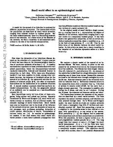
Contributors
Figure 1: An example bipartite graph of Projects and Contributors
properties of the graph were analyzed, followed by a qualitative section to help link the quantitative analysis to subject matter expert experiences.
Collection and Storage
To explore our hypothesis, software project data was collected and analyzed. This data was collected using the freely available FLOSSmole[14] datasets of free and open source projects. Two datasets were analyzed – data from from the popular open source project site Freecode,1 and another from the open source software repository SourceForge.2 The Freecode dataset contained data up to September 2013, while the SourceForge dataset was slightly older with data gathered up to June 2009. Both datasets were chosen because they met two basic criteria: (1) they contained an exhaustive list of projects and contributors to those projects, and (2) they provided some sort of quantitative measure of project “popularity.” This popularity metric will be further described in sections below. Results were analyzed using the Python graph processing package NetworkX[11]. All source code pertaining to the collection and analysis can be found at https://github.com/kevinpeterson/ small-world-effect-research.
2.2
Projects
Analysis
The collected data was organized into a graph structure, with the nodes representing the contributors and the edges representing one or more shared project between contributors. For our purposes, “contributors” includes any person that has been identified as being associated with the project by the project hosting site (Freecode and SourceForge). It is important to note that “contributor” does not always imply code contributions – as issue reporting and documentation, among other things, are valid contributions. Various 1 http://freecode.com/ 2 http://sourceforge.net/
Graph Structure For each dataset, we first considered the dataset to be one large graph. It was observed that the contributor graph was “disconnected,” meaning that there was not a path between all possible nodes. From this large disconnected graph, we extracted a set of connected subgraphs, where each connected subgraph was analyzed. Metrics were then computed for each of these subgraphs. In order to correctly compute the metrics below, a minimum subgraph size was required. Specifically, many of the graph metrics of interest measured “triangles” of nodes and their connections. This implies a subgraph of >= 3 nodes is needed. Because of this, subgraphs of < 3 nodes were not considered for analysis. The contributor/project data can be represented as a bipartite graph. A bipartite graph is a specialized type of graph containing two disjoint sets of verticies. This can be denoted by G = (P, C, E), where P ∩ C = ∅. For our purposes, let set P be the set of all projects, set C be the set of all contributors, and E the edges that connect them. Each project node, therefore, is only connected to contributor nodes, and vice versa, as show in figure 1. In other words, the sets P and C are disjoint. This bipartite representation is typical of what is found in social and collaboration networks[27]. A bipartite graph projection is necessary to further analyze the graph. A bipartite projection involves taking the disjoint node sets P and C, and representing the graph as relationships between only one of those sets of nodes. A projection onto the contributor nodes, or C, of figure 1 is show in figure 2. Here, contributors are connected directly, with edges occurring if a two contributors share one or more common projects. It is important to note that the projection
Page 2
C1 C2 C3
C4
Figure 2: A contributor (C) projection of the figure 1 bipartite graph
Another approach to clustering is to take the average of each node’s local clustering coefficient[33]. To calculate the local clustering coefficient of a node, we follow these steps: Given our graph of nodes C connected by edges E, or G = (C, E), for any given node we can determine its neighborhood (Ni ), or the set of nodes directly connected to a given node. Ni = {vj : eij ∈ E ∧ eji ∈ E ∧ vj ∈ C}
could have been done in terms of the projects, instead of the contributors. This would have led to a graph with nodes of projects P , each being linked by sharing a common contributor. Projection is a common way of representing these bipartite graphs[23], although it is known that bipartite projections are lossy compared to the data represented in the original graph[35]. One of the main sources of information loss is multiple connections between contributors, or contributors that share multiple projects. When doing a bipartite projection based on contributors C, a single link could represent one shared project or many. This is a source of data loss in the projection. The simple approach is to treat one connection the same as many connections between nodes. This is straightforward but lossy[35, 10]. A better approach is to assign a weight to each edge representing repeated links – or in our case – multiple shared collaborators[34, 3]. Graph Analysis To support our hypothesis, there are several key metrics to be studied in regards to the aforementioned graph. Many of these metrics follow the work of Boccaletti et. al [4], and other studies of similar graph types[18, 1]. Clustering Coefficient - Transitivity (C ∆ ) We calculate the Clustering Coefficient (C ∆ ) as a measure of the proportion of closed triangles in a graph[25]: C∆ = 3 ×
number of triangles number of connected triples
This metric shows us how closely related, or “clustered,” that the graph is. It is also the probability that two nodes will be connected if they share a common neighbor[24]. In our context, if contributors C1 and C2 both collaborate with a common contributor C3 , this metric represents the probability that C1 and C2 will collaborate. Clustering Coefficient - Average
(C λ )
Given this neighborhood, we can then calculate how closely connected the nodes are. To do this, we take the number of actual connections between neighbors divided by the total possible number of connections, where ki represents the count of the neighbors of a node, or ki = |Ni | Ciλ =
2|{ejk : vj , vk ∈ Ni , ejk ∈ E}| ki (ki − 1)
From this Local Clustering Coefficient Ciλ , we can then take the average over the entire set of nodes in the graph. 1 X λ Cλ = Ci |C| i∈C
It is important to note that although the terminology is similar[31], C λ and C ∆ are different measurements. Unless otherwise noted, the Transitivity version of this metric (C ∆ ) will be used for all further calculations and metrics. Average Path Length (L) Calculating the Average Path Length (L) allowed us to determine how far removed contributors in the graph are from one another. The path length is calculated as the average distance between any two node pairs in the graph: L=
X 1 λ(vi , vj ) |C| · (|C| − 1) i6=j
Where given vi ∈ C, vj ∈ C, the function λ(vi , vj ) denotes the shortest path between the two nodes. We only considered path length for connected subgraphs, avoiding some complexities of this calculation on disconnected graphs[4]. Small World Quotient (Q) The definition of a small world graph can be formalized by the following equations[15, 31]: First, let γg∆ equal the ratio of the clustering coefficient of a given graph and a random graph. γg∆ =
Cg∆ ∆ Crand
Page 3
1
C ∆ = 0.0
2 4
3 4
C ∆ = 1.0
1
formula for the rank metric could be located for citation. Note that there was no attempt to normalize the two performance metrics between datasets. Because of this, no cross-dataset measurements can be made, as the performance metric is only valid in the context of the enclosing dataset. Qualitative Analysis
3
2 4
3
1
C ∆ = 0.6
2 Figure 3: Example Clustering Coefficient (C ∆ ) values for sample graphs
Next apply a similar pattern to the average path length λg . Lg λg = Lrand Finally, the ratio of the above calculations yields the small world quotient, or Q, of the graph. Q=
γg∆ λg
We assume throughout that any graph exhibiting Q > 1 is a small world graph. Performance To further explore the data, a measurement of project performance was needed. As the explored datasets consisted entirely of open source projects, research indicates that quality, use, user satisfaction, and impact are each possible metrics to measure performance or success[8]. For both datasets, we based our performance metric on use. For Freecode, we used the Popularity Score metric, which is calculated by the following formula:3 ((record hits + U RL hits) · (f ollowers + 1))1/2 For the SourceForge dataset, performance was based on the repository’s internal rank metric. This metric ranks each project from 1 to the total number of projects in SourceForge (Psf ), or 1