of resellers were willing to construct the nodes to our specifications (see Table 2.1) and deliver the .... perl script comes to the rescue. sseq simply creates a string of node names. ..... First, particles are domain decomposed into spatial groups.
The Space Simulator Michael S. Warren, Chris Fryer and M. Patrick Goda Theoretical Astrophysics Los Alamos National Laboratory Los Alamos, New Mexico No Institute Given The Space Simulator is a 294-processor Beowulf cluster with theoretical peak performance just below 1.5 Teraflop/s. It is based on the Shuttle XPC SS51G mini chassis. Each node consists of a 2.53 GHz Pentium 4 processor, 1 Gb of 333 MHz DDR SDRAM, an 80 Gbyte Maxtor hard drive, and a 3Com 3C996B-T gigabit ethernet card. The network is made up of a Foundry FastIron 1500 and 800 Gigabit Ethernet switch. Each individual node cost less than $1000, and the entire system cost under $500,000. The cluster achieved Linpack performance of 665.1 Gflop/s on 288 processors in October 2002, making it the 85th fastest computer in the world according to the 20th TOP500 list. Performance has since improved to 757.1 Linpack Gflop/s. In this paper we describe the design, implementation and performance of the cluster, as well as some scientific application results obtained with the machine.
1
Introduction
The Space Simulator [1] is our third generation Beowulf cluster. The first was Loki [2], which was constructed in 1996 from 16 200 MHz Pentium Pro processors for $50k. Loki was among the earliest generation of Beowulf clusters [3], and was the first to be recognized with the Gordon Bell price/performance award [4]. Loki was followed by the Avalon cluster [5], which used 144 alpha processors and cost about $300k. Avalon also won a Gordon Bell price/performance prize [6] and was ranked as the 113th fastest computer in the world in June 1998 [7]. The Space Simulator follows the same basic architecture as our previous machines, but is the first to use Gigabit Ethernet as the network fabric, and requires significantly less space than a cluster using typical ATX sized cases. The process by which we designed the machine and selected components is briefly described in section 2.1. We also discuss the way we installed Linux on each processor, and the power consumption and reliability of the cluster in sections 2.2 and 2.4. We mention the software environment of the cluster and several of the software tools that we have developed in section 3. The CPU and network performance of the cluster on a variety of benchmarks is explored in section 4. We then discuss the particular astrophysics applications the cluster was designed for in section 5. We conclude with a comparison of the capabilities of the Space Simulator with the similar architecture of the Loki cluster from exactly six years prior.
2
Zen and the Art of Beowulf
Instruction #1 — Assembly of Beowulf requires great peace of mind.
2 Warren, Fryer & Goda
Fig. 1. The Space Simulator resides on five sets of 14x48 inch wire shelves with 86 inch posts. Each rack holds 55 processing nodes, in 11 rows of 5 nodes each. Shown here are portions of the front two racks. The additional three racks are located behind these, facing in the opposite direction. This results in the air heated by the systems being exhausted into the channel between the rows of shelves. The aisle between the rows of shelves is 44 inches wide, resulting in an overall width of 6 feet and a length of 12 feet
The Space Simulator 3
Fig. 2. This image shows MPG in the area between the rows of processing nodes. In the picture you can see a power strip with 10 power cords which supplies the power for one shelf of nodes, as well as the blue Gigabit Ethernet cables connected to each node
4 Warren, Fryer & Goda
Fig. 3. A front view of the Space Simulator which shows the rack containing the two Foundry Gigabit Ethernet switches. The fiber trunk between the two switches are the orange cables in the picture. The 224 ethernet cables attached to the lower switch obscures the upper half of the Foundry 1500 switch, while the Foundry 800 switch is mounted on the top portion of the rack
The Space Simulator 5 2.1
Designing and Building the Cluster
It is possible to enumerate a set of guidelines about how to construct a Beowulf, filled with details about disks and CPUs and network performance. However, since the components available change so rapidly, anything more than general statements about design become stale after a month or two. The funds to purchase the Space Simulator became unexpectedly available in midJuly of 2002. Fiscal constraints required the system to be delivered by September 31. This left little time for benchmarking systems and testing components, and the architecture of the Space Simulator was defined by mid-August of 2002, based on the Shuttle XPC chassis suggested by R. Fryer of BEOMAX. Our goal was to obtain a computer which would obtain the highest performance possible on the astrophysics codes we wanted to run, within the budget we were alloted. It had to be delivered within one month. The machine also had to be reliable and maintainable enough that our very limited system administration resources would be capable of keeping the machine operational. The power constraints were contained mostly in the amount of cooling available in our machine room. An upgrade to the cooling system would have been very expensive and take a long time. We estimated the amount of cooling capacity available would limit the cluster to about 35 kW of power dissipation. There were also constraints on the number of amps available through our power distribution unit. To maximize the power available, one of our specifications required the use of power factor corrected (PFC) power supplies. Typical PC power supplies we measured had a power factor of .66 or less, which meant that current loads were higher than necessary. PFC power supplies have a power factor of 0.99, placing the voltage and current in phase and maximizing the efficiency of the power delivery system.
Table 1. Space Simulator architecture and price (September, 2002). The total cost per node was $1646, with $728 (44%) of that figure representing the Network Interface Cards and Ethernet switches Qty. 294 294 588 294 294 294
Price 280 254 118 95 83 35
1 Total
Ext. Description 82,320 Shuttle SS51G mini system (bare) 74,676 Intel P4/2.53GHz, 533MHz FSB, 512k cache 69,384 512Mb DDR333 SDRAM (1024Mb per node) 27,930 3com 3c996B-T Gigabit Ethernet PCI card 24,402 Maxtor 4K080H4 80Gb 5400rpm Hard Disk 10,290 Assembly Labor/Extended Warranty 4,000 Cat6 Ethernet cables 3,300 Wire shelving/switch rack 1,378 Power strips 186,175 Foundry FastIron 1500+800, 304 Gigabit ports $483,855 $1646 per node 5.06 Gflop/s peak per node
6 Warren, Fryer & Goda Given that power and space limited us to the neighborhood of 300 processors, we were able to afford a large gigabit ethernet switch. It is possible that if we were able to cool more processors we might have thought harder about ways to connect the machines together more cheaply (with a tree of trunked 36-port 3com switches, for example), which would have allowed a larger machine, albeit with a more complex topology. However, since the cooling constraint existed, it made the decision to spend over 40% of our budget on the network easier. We obtained quotes for clusters from several manufacturers. While one can argue the specifics of the value of extras typically included in such clusters (high-performance interconnects, dual-CPU motherboards, system management features), we estimated that a “commercial” solution would provide about 50% of the performance of what we could build ourselves, for the same amount of money. For many customers, this would be an acceptable markup. Certainly, it is a vast improvement over the factor of 10 difference that was typical between a self-built Beowulf cluster and the available commercial solutions 5 years ago. Some would say that the biggest advantage to a commercial solution is less risk that something will not work. The less tangible price you pay is that the hardware typically lags somewhat behind the state-of-the-art. This is sensible, in that it takes some time to integrate a commercial system and thoroughly test the interoperability of the components. However, even commercial solutions are not perfect, and it is inevitable that some time will need to be spent identifying problems which have developed during transport of the machine from the factory, or fixing software problems that are only discovered once production computing begins. The second major factor in our decision to build the system ourselves was that we were not confident that any of the cluster vendors could deliver a system with only one month lead time, especially at the end of the government fiscal year. Given this time constraint, we were prepared to actually buy parts and assemble the computing nodes ourselves if there was no other way to meet the delivery deadline. Fortunately a number of resellers were willing to construct the nodes to our specifications (see Table 2.1) and deliver the systems on time. Deciding on exactly what to buy was not a simple process. Resellers would only sell in large volumes, and it proved impossible to obtain a prototype Shuttle system due to organizational bureaucracy. In the end, several conventional ATX systems with both P4 and Athlon processors, using DDR SDRAM and RDRAM were purchased through normal procurement channels, and a Shuttle mini system was bought by one of the authors using his own credit card. Using these prototypes, we were able to determine that our codes ran faster on the P4 systems, the RDRAM did not improve the results enough to justify its cost, and that the 3com ethernet card performed much better than other cards in the Shuttle systems. We wrote a detailed specification for the purchase, and it was submitted for bids on August 15. On August 29, MA Labs was awarded the contract for the processing nodes, and Integrity Networking Systems was awarded the contract for the Foundry switches. We requested that 16 systems ship as soon as possible, with express delivery, so that we could test the actual components being used before the entire cluster was assembled. Systems began to arrive on September 12. We discovered some performance inconsistencies in these systems that were traced to the fact that the CPU temperatures
The Space Simulator 7 were much hotter than the prototype system. After disassembling one of the systems, it was determined that there was no heat sink compound between the processor die and the heat pipe. This was pointed out to the vendor, who corrected the problem on the remaining systems. The final processing nodes and the Ethernet switches arrived on September 26. Our assembly task was simply to unpack the nodes and plug in the power and ethernet cables, and then remotely install the OS. The most labor intensive part of the whole process was unpacking the cat6 ethernet cables. The only cat6 cables we could find were manufactured by Belkin, and were coiled in their packaging very tightly, which made them difficult to unravel, and prone to tangling with other cables. An useful lesson re-learned was to clearly label the cables on each end with the processor number before plugging them in to the nodes and the switches. On September 30, a Linpack result of 430 Gflop/s was obtained on 208 processors. This improved to 527 Gflop/s on 240 processors by Oct. 5, 622 Gflop/s on 272 processors on Oct. 16, and our TOP500 result of 665.1 Gflop/s on 288 processors on October 30. 2.2
Space and Power consumption
Table 2. Power consumption for various cluster configurations running the parallel N-body code. Note that power figures include power consumption of NIC and network switch. The P4 figures listed in column three represent the higher power consumed by the previous generation of processors. The P4 figures in column 5 are for the Space Simulator, and the higher performance there is primarily due to extra optimization from the Intel icc compiler vs gcc used for column 3 Processor Athlon P4 P3 P4 TM5600 TM5800 Clock (MHz) 1800 2200 1133 2530 667 933 Performance (Mflop/s) 952 656 595 1357 298 373 Power (watts/proc) 160 130 70 125 22 24 Power efficiency (Mflop/s/watt) 5.95 5.05 8.5 10.8 13.5 15.5
The entire cluster consumes about 35 kilowatts of power while under load. This falls to 21 kilowatts when idle. The maximum power consumption we have measured on a processing node is 110 watts, while running the Linpack benchmark The cost of electricity for the machine works out to about $30k per year. With space charges at Los Alamos of about $50 per square foot, the charge for the space to put the machine adds an additional $4k per year. Scaling the purchase price by Moore’s Law, when the machine is about 6 years old, it will cost more per year for power and space than the value of the computation produced by the machine. This puts a clear upper limit on its useful lifetime. We have calculated the power consumption of our code on a variety of systems, and offer the statistics in Table 2 by way of comparing the SS to other architectures. Note
8 Warren, Fryer & Goda that the power efficiency of a bladed Transmeta cluster is superior to that of the Space Simulator, but it does not scale to the same total performance [8].
Fig. 4. A smoothed representation of the temperature across the cluster obtained from the lm sensors package on each node. The air conditioning unit is located on the left side of each set of racks, with the intake at the bottom and the outflow at the top. The left edge of racks 1 & 2 and the left edge of racks 3, 4 & 5 are located equidistant from the AC, with their backs facing inward. The cooler temperatures near the cold air are evident. A hot spot due to warm air rising and limited convection on the right side of racks 3, 4 & 5 is also clearly seen. Note that the absolute temperature scale shown here may be in error, since the data sheets for the sensors used in our nodes are unavailable, and thus are not well supported by the lm sensors package. An independent measure of system temperatures is provided by reading the hard drive temperature via smartctl. These temperatures range from 20-40 degrees C, and follow a similar spatial pattern
2.3
OS install
We used the PXE functionality of our NICs along with pxelinux and RedHat kickstart to install Linux on each node. We encountered several problems during this process. By default, 3Com NICs do not have PXE enabled. You are required to execute a DOS utility to enable the card to do PXE. The only way to do that is to manually boot DOS and run the utility. One of the tasks we specified that the reseller perform was to do this process for each NIC. Out of the 294 nodes, about 10 were not PXE enabled. They would fail during the OS install, which required us to remove the NIC and place it in a machine with a floppy drive to execute the utility to enable PXE. Second, bootp and DHCP requests would sometimes work, and sometimes fail. These requests were issued several times during the install process, and would always work when issued from the NIC, but usually fail during the intermediate stages when issued from the RedHat installer. We determined that the problem was due to the spanning tree protocol in the network switch, which would cause these broadcast requests
The Space Simulator 9 to time out if they were not given sufficient time to complete. Disabling spanning tree in the switch fixed the problem. The last problem was that we were unable to get pxelinux installs to work with RedHat 8.0 (then in beta). RedHat 7.3 worked fine. A brief investigation was unable to determine the problem, and it was decided that RedHat 7.3 would be sufficient. We have since re-installed RedHat 9.0 on the whole cluster via pxelinux without a problem. The use of pxelinux to boot has several advantages. One of the nicer features is the ability to boot a variety of system images. We are able to boot the “memtest86” utility directly over the network to verify memory problems, without the need for a floppy or CD-ROM on each node. Additionally, we plan to use this functionality to upgrade the BIOS on each node if it becomes necessary. Doing BIOS upgrades was really the only reason to have a floppy disk on every node, so the ability to use pxelinux to boot a DOS image over the network allowed us to dispense with the floppy drives on the SS. The nodes are named s00, s01, ..., s293, and the names are mapped to their MAC address in /etc/dhcpd.conf. This map is generated by a perl script using the diagnostic output of the ethernet switch, thereby allowing us to keep the topology of the switch ports associated with the physical location of the nodes in the racks. 2.4
Reliability
In our experience, the component most likely to fail in a cluster are the fans. We expect somewhat increased reliability from the SS cluster compared with our previous clusters, since the CPU fan is eliminated by the heat pipe used in the Shuttle chassis. During the installation of the cluster and the initial large Linpack benchmark runs we identified the following defective hardware: 3 power supplies 6 sticks of DRAM
6 disk drives 1 ethernet card
4 motherboards
During the six month period since the initial failures, the following hardware has failed: 2 power supplies 3 sticks of DRAM
5 disk drives 1 motherboard 1 fan connector loose
It is possible that the faulty DRAM and motherboard/CPU discovered after the initial installation was defective to begin with, but took longer to identify since the errors were very infrequent. Additionally, there have been less than 10 “soft” node errors, which resolved themselves, or did not occur again after the node was rebooted. One perhaps interesting anecdote is that on every occasion where a node has failed with a Linux kernel panic, the cause was traced to bad hardware. The entire cluster has gone down on two occasions, once when the 120 kVa power distribution unit for the machine room failed and had to be replaced, which resulted in three days of down-time, and once during a power outage which lasted about 1 hour. On several other occasions, 15-amp breakers on individual power strips tripped, necessitating a rebalancing of the power distribution using a slightly more conservative maximum power consumption figure.
10 Warren, Fryer & Goda Additionally, there have been 4 soft failures of ports on the ethernet switch which were resolved by a power cycle of the switch.
3
Software Environment and Tools
Our basic philosophy has been “simpler is better” in terms of tools to manage parallel machines. We have been quite productive using a stock RedHat installation, with the addition of a message passing library such as MPICH or LAM (and LAM now comes with RedHat), and the scripts and libraries in the subsections below. Some codes will benefit from the architecture specific optimizations available with the Intel or Portland Group C and Fortran compilers, but we have found software development and cluster management tools beyond that can often be more trouble than they are worth. In particular, we have intentionally avoided installing software such as batch schedulers, since the small user base on the Space Simulator machine can much more effectively manage the resources by an exchange of e-mail. 3.1
Prsh
Prsh is a script developed by J. Salmon which implements a ”parallel” rsh. Prsh runs a command on a list of remote processors with optional timeouts, output flushing, status reports, etc. It is implemented with about 200 lines of perl. It has turned out to be a tremendously powerful and flexible way to extend the usual UNIX command-line interface across a parallel machine. A typical prsh command would be: prsh -- uptime This shows the uptime on nodes defined by the environment variable PRSH_NODES. The last argument to prsh can be any valid command you would ordinarily give on the command-line. ls, cp, shutdown, killall, date, etc. A more explicit way to specify nodes may also be used: prsh s00 s01 s02 s03 -- uptime Typing machine names quickly becomes tiresome on a large machine, but another small perl script comes to the rescue. sseq simply creates a string of node names. The example above is equivalent to prsh ‘sseq 0 3‘ -- uptime, which is not much shorter than the explicit command, but prsh ‘sseq 0 293‘ -- shutdown -h certainly is. Prsh calls rsh asynchronously, so all commands execute in parallel. The prsh command in practice feels very responsive, with commands running across 288 SS processors completing in less than 2 seconds. prsh also can be told to use ssh as an option, so all system maintenance commands are performed using ssh-agent authentication and prsh from the front-end. 3.2
SWAMPI
Since about 1990 we have maintained a small message passing library which we have used to run our parallel codes on networks of workstations. The library was initially implemented with UDP, since UDP performance on the machines and operating systems at that time was much superior to TCP performance. The library implemented only about
The Space Simulator 11 10 basic communication functions, but those were sufficient to run our parallel codes, since we believed (or soon discovered) that depending on anything beyond the basics would not run reliably on most parallel machines. With the discovery that Linux TCP bandwidth over fast ethernet was equivalent to UDP performance, we were able to substantially simplify our simple message passing library (since we no longer had to handle message sequencing and retries ourselves). While doing this we also took the opportunity to align the code more closely with the MPI standard. This rewrite was done during a couple of weeks in early 1997. This library (named SWAMPI) is implemented in about 2000 lines of code, and implements the 24 most commonly used MPI functions. This may be contrasted with many more lines of code in the LAM [9] implementation and MPICH distribution [10]. Needless to say, it is considerably easier to understand what is happening in 2000 lines of our own code vs 100,000 of somebody else’s. SWAMPI has been used on the SS, showing increased reliability and performance over MPICH. Our more recent experiences with the LAM implementation of MPI on the SS have shown that it in most cases matches or exceeds the performance of SWAMPI, so SWAMPI’s interest to a more general audience is likely limited.
4
Benchmarks
In this section, we attempt to characterize the performance of the Space Simulator, proceeding from micro-benchmarks of particular aspects of the architecture to more general measurements. In particular, we try to provide a clear baseline for the measurement of gigabit-ethernet connected clusters, and provide a basis for future comparison with clusters connected via less mainstream technology. In particular, these benchmark results can begin to point one in the right direction for answering questions like “Which compiler is fastest?” and “Which MPI implementation should I use?” 4.1
Network Performance
Gigabit network performance varies dramatically depending on the particular NIC used in the Shuttle systems. Some cards which had very good performance on a 64-bit or 66 MHz PCI bus performed poorly with the Shuttle 32-bit 33 MHz bus. We selected the 3Com 3c996B-T cards based on testing a variety of cards on a prototype system. The performance results are listed below using Linux 2.4.20. The 1.0 version of the tg3 driver that shipped with Linux 2.4.20 turned out to be significantly slower than earlier versions, so the results below use the earlier 0.99 version. In order to determine the behavior of the Foundry switch backplane, we wrote a small MPI program which simultaneously sends messages between pairs of processors along various hypercube edges. Within a 16-port switch module, the messages are nonblocking. The capacity from one module to another is only 8 gigabits. We verified that with 16 processors on one module sending to 16 modules on another module, the total throughput was about 6000 Mbits. Further, since our overall switch is a trunked combination of a Fastiron 1500 and a Fastiron 800, messages between the two switches are limited by the 8 Mbit trunk. This limits the scaling of codes running on more than about 256 processors.
12 Warren, Fryer & Goda 800
700
Bandwidth in Mbps
600
"TCP" "LAM-O" "SWAMPI" "LAM" "mpich2-0.92" "mpich-1.2.5"
500
400
300
200
100
0 1
10
100
1000 10000 Message Size in Bytes
100000
1e+06
1e+07
Fig. 5. We show bandwidth vs message size for a variety of message passing libraries as measured via NetPIPE [11]. Several features are evident, showing mpich-1.2.5 has lower performance for large messages than the rest of the libraries. The 0.92 beta release of mpich2 has apparently solved that problem. Also, using LAM 6.5.9 with the -O flag (designating a homogeneous environment) significantly improves performance. The highest bandwidth is obtained via plain TCP, achieving 779 Mbits/sec. The latencies for small messages range from 79 microseconds for TCP, to 83 microseconds for LAM, and 87 microseconds for mpich-1.2.5 and mpich2-0.92
4.2
Memory Bandwidth
The node memory bandwidth is less than optimal for its 333 MHz frequency due to the fact that the on-board video system uses the system DRAM for it’s frame buffer. It is possible to disable the on-board VGA controller and increase memory copy bandwidth by 14%, but you must then insert an AGP video card into the system in order for it to boot. Stream [12] results for the nodes in their normal configuration with a 4 MByte shared VGA frame buffer are: Function Copy: Scale: Add: Triad: 4.3
Rate (MB/s) 1144.5249 1145.2130 1262.9053 1265.4891
RMS time 0.0700 0.0699 0.0951 0.0949
Min time 0.0699 0.0699 0.0950 0.0948
Max time 0.0702 0.0700 0.0951 0.0949
Linpack
In contrast to commercial machines which use a variety of proprietary libraries and compilers to obtain their peak performance, our Linpack benchmark result of 665.1
The Space Simulator 13
Fig. 6. The Space Simulator ranks at #85 on the 20th TOP500 list of the fastest computers in the world, as determined by the Linpack benchmark. Performance of 665.1 Gflop/s was obtained on 288 processors in October 2002. In April 2003, we obtained a higher figure of 757.1 Gflop/s through the use of a slightly faster version of ATLAS and using LAM instead of mpich. This performance would have ranked the Space Simulator at #69 on the 20th TOP500 list. We believe our results are the first example of a machine in the TOP500 with price/performance of better than 1 dollar per Mflop/s (we obtain 63.9 cents per Mflop/s, or $639 per Gflop/s)
Gflop/s was obtained using freely available software and commodity off-the-shelf hardware. The OS (RedHat 7.3), kernel (Linux 2.4.20), message passing library (MPICH), compiler (gcc 3.1.1), BLAS library (ATLAS) and the High Performance Linpack (HPL) software are all freely available. This Linpack result ranks us as the 85th fastest computer in the world on the November 2002 TOP500 list [13]. ========================================================================= T/V N NB P Q Time Gflops ------------------------------------------------------------------------W25R2C4 180000 160 16 18 5845.59 6.651e+02 ------------------------------------------------------------------------||Ax-b||_oo / ( eps * ||A||_1 * N ) = 0.0042969 ...... PASSED ||Ax-b||_oo / ( eps * ||A||_1 * ||x||_1 ) = 0.0089214 ...... PASSED ||Ax-b||_oo / ( eps * ||A||_oo * ||x||_oo ) = 0.0014673 ...... PASSED =========================================================================
In April 2003, the Linpack benchmarks were run again on 288 processors. Instead of MPICH 1.2.4, we used LAM 6.5.9 as the MPI implementation. In addition, the somewhat newer ATLAS 3.5.0 distribution was used for the level 3 BLAS, and the Intel 7.1 compiler suite was used to compile HPL (while gcc was used for ATLAS). The significant improvement seen, from 665.1 Gflop/s to 757.1 Gflop/s, we believe was mostly
14 Warren, Fryer & Goda due to the switch to LAM. The exact results of running the benchmark 8 times in a row (which all passed the residual check) are as follows: ========================================================================= T/V N NB P Q Time Gflops ------------------------------------------------------------------------W25R2C4 180000 160 16 18 5153.50 7.544e+02 W25R2C4 180000 160 16 18 5150.74 7.549e+02 W25R2C4 180000 160 16 18 5146.35 7.555e+02 W25R2C4 180000 160 16 18 5135.46 7.571e+02 W25R2C4 180000 160 16 18 5160.75 7.534e+02 W25R2C4 180000 160 16 18 5191.60 7.489e+02 W25R2C4 180000 160 16 18 5177.24 7.510e+02 W25R2C4 180000 160 16 18 5159.14 7.536e+02 =========================================================================
4.4
Gravity Kernel Performance
Execution time for our parallel N-body application is dominated by the force calculation in the inner loop. We have collected performance figures on a variety of processors in Table 4.4. The SS results correspond to the 2530-MHz Intel P4. Table 3. Mflop/s obtained on our gravitational micro-kernel benchmark. The first column uses the math library sqrt, the second column uses an optimization by Karp [14], which decomposes the reciprocal square root into a table lookup, Chebychev interpolation and Newton-Raphson iteration, which uses only adds and multiplies. Note the significant improvement obtained through the use of the Intel version 6.0 compiler, which enables the P4 SSE and SSE2 capabilities Processor 533-MHz Alpha EV56 667-MHz Transmeta TM5600 933-MHz Transmeta TM5800 375-MHz IBM Power3 1133-MHz Intel P3 1200-MHz AMD Athlon MP 2200-MHz Intel P4 2530-MHz Intel P4 1800-MHz AMD Athlon XP 1250-MHz Alpha 21264C 2530-MHz Intel P4 (icc)
4.5
libm 76.2 128.7 189.5 298.5 292.2 350.7 668.0 779.3 609.9 935.2 1170.0
Karp 242.2 297.5 373.2 514.4 594.9 614.0 655.5 792.6 951.9 1141.0 1357.0
NAS parallel benchmarks
The results shown in Tables 4.5 and 4.5 use the NAS Parallel benchmarks version 2 [15]. These benchmarks, based on Fortran 77 and the MPI standard, are intended to
The Space Simulator 15 approximate the performance a typical user can expect for a portable parallel program on a distributed memory computer. All results use the Intel version 7.1 compilers with FFLAGS = -O3 -tpp7 -xW -ipo -fno-alias and LAM 6.5.9 as the message passing library. Table 4. NAS 2.4 benchmark performance per processor for runs ranging in size from 1 processor to 289 processors. Some of this data is plotted in Figures 7 and 8 N procs 1 2 4 8 9 16 25 32 36 49 64 81 100 121 128 144 169 196 225 256 289
5 5.1
BT A B C 331
D
SP A B C 217 221
304 311
181 190 209
280 296 304 265 280 296 266 270 287
140 178 195 158 160 180 169 127 168
252 238 227 227 217 213
263 236 210 192 173 166
279 151 119 272 127 108 266 106 98 260 292 92 81 249 291 73 77 250 288 67 70
177 161 133 115 72 37
174 197 157 164 123 135
247 223 198 186 160 247
282 275 270 264 246
53 48 40 34 24 13
82 77 52 56 37 16
102 144 122 117 107 102 89 85 71 75 62 41
D
A 410 397 389 452
LU MG B C D A B C D 413 419 392 416 406 408 373 396 397 401 327 349 404 371 383 308 333 389
458 415 369
271 287 360
360 440 352
242 254 329
172 271 393 436 358 214 225 267 175 173 165 137 267 400 358 124 144 246 344 160 154 138 96 114 61 166 299 318 44 48 72 110
Applications N-body methods
N-body methods are widely used in a variety of computational physics algorithms where long-range interactions are important. Several methods have been introduced which allow N-body simulations to be performed on arbitrary collections of bodies in time much less than O(N 2 ), without imposition of a lattice [16, 17]. They have in common the use of a truncated expansion to approximate the contribution of many bodies with a single interaction. The resulting complexity is usually determined to be O(N) or O(N log N), which allows computations using orders of magnitude more particles. These methods represent a system of N bodies in a hierarchical manner by the use of
16 Warren, Fryer & Goda
Table 5. NAS 2.4 benchmark performance per processor for runs ranging in size from 1 processor to 256processors. Some of this data is plotted in Figures 7 and 8 N procs 1 2 4 8 16 32 64 128 256
A 298 239 161 117 76 45 24 14 4
CG B C 58 106 52 110 50 134 101 89 76 67 85 38 51 32 38 14 9
D A 343 233 202 178 142 77 23 61 29 5 19 5
FT B C D A 12.6 12.6 209 12.6 189 12.6 172 193 12.6 155 159 12.4 118 154 12.2 84 151 12.1 21 79 85 12.0
EP B C 12.7 12.6 12.6 12.6 12.6 12.6 12.6 12.6 12.6 12.6 12.6 12.5 12.6 12.4 12.5 12.2 12.4
D
A 27.90 13.90 10.60 6.15 2.68 12.6 0.85 0.35 12.6 0.24 12.6 0.04
IS B 26.44 13.65 10.71 8.84 6.20 3.01 0.78 1.08 0.03
C
10.48 9.11 7.71 5.75 3.62 0.15
Fig. 7. Scaling of the NAS 2.4 Class D benchmarks on the Space Simulator. Perfect scaling would be a straight horizontal line for the plot on the right. Data for this plot are contained in Tables 4 and 5
The Space Simulator 17
Fig. 8. Scaling of the NAS 2.4 Class C benchmarks on the Space Simulator. The computational problems are smaller than the Class D results shown in the previous plot, so the scaling is not as good for large numbers of processors. The feature in the plot for the LU benchmark (where the performance per processor becomes more higher on 64 processors than on a single processor) is likely due to the problem being divided into enough pieces that it fits into L2 cache on the processor
a spatial tree data structure. Aggregations of bodies at various levels of detail form the internal nodes of the tree (cells). These methods obtain greatly increased efficiency by approximating the forces on particles. Properly used, these methods do not contribute significantly to the total solution error. This is because the force errors are exceeded by or are comparable to the time integration error and discretization error. Using a generic design, we have implemented a variety of modules to solve problems in galactic dynamics [18] and cosmology [19] as well as fluid-dynamical problems using smoothed particle hydrodynamics [20], a vortex particle method [21] and boundary integral methods. 5.2
The Hashed Oct-Tree Library
Our parallel N-body code has been evolving for over a decade on many platforms. We began with an Intel ipsc/860, Ncube machines, and the Caltech/JPL Mark III [22, 18]. This original version of the code was abandoned after it won a Gordon Bell Performance Prize in 1992 [23], due to various flaws inherent in the code, which was ported from a serial version. A new version of the code was initially described in [24]. The basic algorithm may be divided into several stages. Our discussion here is necessarily brief. First, particles are domain decomposed into spatial groups. Second, a distributed tree data structure is constructed. In the main stage of the algorithm, this tree is traversed independently in each processor, with requests for non-local data being generated as needed. In our implementation, we assign a Key to each particle, which is based on Morton ordering. This maps the points in 3-dimensional space to a 1-dimensional list, which maintaining as much spatial locality as possible. The domain decomposition
18 Warren, Fryer & Goda Table 6. Historical Performance of Treecode Year 2003 2003 2002 2002 2000 1998 1996 1996 1996 1995 1995 1993
Site Machine Procs Gflop/s Mflops/proc LANL ASCI QB 3600 2793 775.8 LANL Space Simulator 288 179.7 623.9 NERSC IBM SP-3(375/W) 256 57.70 225.0 LANL Green Destiny 212 38.9 183.5 LANL SGI Origin 2000 64 13.10 205.0 LANL Avalon 128 16.16 126.0 LANL Loki 16 1.28 80.0 SC ’96 Loki+Hyglac 32 2.19 68.4 Sandia ASCI Red 6800 464.9 68.4 JPL Cray T3D 256 7.94 31.0 LANL TMC CM-5 512 14.06 27.5 Caltech Intel Delta 512 10.02 19.6
is obtained by splitting this list into N p (number of processors) pieces (see Figure 9). The implementation of the domain decomposition is practically identical to a parallel sorting algorithm, with the modification that the amount of data that ends up in each processor is weighted by the work associated with each item. The Morton ordered key labeling scheme implicitly defines the topology of the tree, and makes it possible to easily compute the key of a parent, daughter, or boundary cell for a given key. A hash table is used in order to translate the key into a pointer to the location where the cell data are stored. This level of indirection through a hash table can also be used to catch accesses to non-local data, and allows us to request and receive data from other processors using the global key name space. An efficient mechanism for latency hiding in the tree traversal phase of the algorithm is critical. To avoid stalls during non-local data access, we effectively do explicit “context switching” using a software queue to keep track of which computations have been put aside waiting for messages to arrive. In order to manage the complexities of the required asynchronous message traffic, we have developed a paradigm called “asynchronous batched messages (ABM)” built from primitive send/recv functions whose interface is modeled after that of active messages. All of this data structure manipulation is to support the fundamental approximation employed by treecodes:
∑ j
Gm j d i j GMd i,cm ≈ +..., 3 |di j |3 di,cm
(1)
where d i,cm = xi − xcm is the vector from xi to the center-of-mass of the particles that appear under the summation on the left-hand side, and the ellipsis indicates quadrupole, octopole, and further terms in the multipole expansion. The monopole approximation, i.e., Eqn. 1 with only the first term on the right-hand side, was known to Newton, who realized that the gravitational effect of an extended body like the moon can be approximated by replacing the entire system by a point-mass located at the center of mass.
The Space Simulator 19
Fig. 9. On top is the self-similar curve used for load-balancing, while the lower figure represents a tree data structure in 2d for a group of centrally condensed particles
20 Warren, Fryer & Goda Effectively managing the errors introduced by this approximation is the subject of an entire paper of ours [25]. In Table 6 we show the performance of the Space Simulator on a standard simulation problem which we have run on most of the major supercomputer architectures of the past decade. The problem is a spherical distribution of particles which represents the initial evolution of a cosmological N-body simulation. Overall, the performance of the full Space Simulator cluster is similar to that of 256 processors on ASCI Q, or a 1024 processor SP-3. 5.3
Cosmology Simulations
Fig. 10. The figure represents a portion of the Universe about 125 Megaparsecs on a side at a redshift of 0.3, or an age of 3.5 billion years prior to the present epoch. The overall simulation of about 700 timesteps used 134 million particles, and was completed in a single run of just over 24 hours on 250 processors of the Space Simulator. 1.5 Terabytes of data from this simulation was saved
Obtaining a quantitative understanding of galaxy formation and clustering is the most important open theoretical problem in the study of the large-scale structure of the
The Space Simulator 21 Universe. Observations strongly support the theoretical paradigm that structure evolves through gravitational collapse of primarily dark matter. The revolutionary transformation of cosmology from a qualitative to a quantitative science has occurred over just the last fifteen years. Driven by a powerful and diverse suite of observations, the parameters describing the large-scale Universe are now known to extraordinary precision. Structure in the Universe forms almost entirely due to the gravitational collapse of primordial density fluctuations. On the very largest scales, such as those characteristic of the microwave background, linear theory is applicable; with the addition of a small amount of thermodynamics and linearized gas dynamics, a quantitative understanding has been achieved. At smaller scales, the essential nonlinearity of gravitational collapse makes such an understanding much harder to attain. In this regime, the distribution of matter can be studied only via large scale N-body simulations. Our recent N-body simulations have achieved unprecedented spatial and mass resolution. Simulations at this resolution allow us to examine the sub-structure of dark matter halos and approach the problem of galaxy formation in a very direct way, possibly resolving many of the problems posed by bias, both in galaxy position and velocity fields. We are currently performing several 134 million particle cosmological N-body simulations per week on the Space Simulator, and have mostly completed a run with over 1 billion particles. Even larger simulations are possible using the out-of-core version of our code [26]. 5.4
Core-Collapse Supernovae
Core-collapse supernovae play a vital role in nearly every aspect of astronomy both as major sources of the emission of gamma-rays, neutrinos and gravitational waves to the chemical enrichment of the universe and the formation of compact objects (black holes, neutron stars, quark stars). These explosions are driven by neutrinos emitted from the collapsed core of a massive star. Studying core-collapse supernovae requires the coupling of gravitational and pressure forces of the core as it collapses down to nuclear densities with the radiation effects from neutrinos — a true radiation/hydrodynamics problem. The combination of radiation transport and the complex description of pressure forces for matter at nuclear densities pose difficulties both in optimization and message passing. In addition, these simulations must be run for 0.1-0.2 million timesteps. Because of these difficulties, nearly all previous simulations of these events have been limited to 2-dimensions. Fryer, Warren and collaborators have performed the first ever full-physics threedimensional simulations of supernova core-collapse [27] as part of the DOE SCIDAC Supernova Science Center http://www.supersci.org. By implementing the smooth particle hydrodynamics formalism onto the tree structure described above for N-body studies, we have been able to include both the essential physics and a flux-limited diffusion algorithm to model the neutrino transport. The largest simulation using 5 million particles was finished recently, and required roughly one month of time to model 100,000 timesteps on a 256 processors of the ASCI Q system. Taking advantage of the Lagrangian nature of smooth particle hydrodynamics, we have begun to study global asphericities in core-collapse: rotation (Figs. 11, 12) and asymmetric collapse (Fig. 13). These 3-dimensional simulations allow us to address a number of outstanding questions
22 Warren, Fryer & Goda in core-collapse astrophysics such as the origin of neutron star kicks and the gravitational wave signal for stellar collapse (Fig. 13). We are currently performing several follow-up simulations on the Space Simulator. For our 1 million particle simulations on 128 processors, per processor performance (using gcc/g77) is about 1/2 that of the ASCI Q system. We are running several simulations using 32 processors out to 150,000 timesteps. These simulations take roughly 4 months. Performance tuning remains to be done, especially investigating the use of the Intel 7.0 compilers.
6
Conclusion
Beowulf clusters have proven to be an effective computing resource in many appplication areas. We have demonstrated that commodity PC technology coupled with the latest generation of high-volume ethernet technology is capable of supercomputer-class performance. It is interesting to note there have been exactly six years between the completion of the Loki and Space Simulator clusters, which results in four “Moore’s Law” doublings. Comparing the Loki architecture and price in Table 7 to the Space Simulator, we can see that Moore’s Law scaling has actually been greatly exceeded in some aspects of the architecture. For instance, in 1996, Loki’s disks cost $111 per Gigabyte. For the SS, they are close to $1 a Gigabyte, which is a factor of seven beyond the factor of 16 from Moore’s Law over six years. For memory, in the Loki days it was $7.35 per Megabyte, and is now 23 cents per Megabyte, 2x lower than Moore’s Law would have predicted. Qty. 16 16 16 64 16 16 16 16 16 2
Price 595 15 295 235 359 85 129 59 119 4794
Total
Ext. Description 9520 Intel Pentium Pro 200 Mhz CPU/256k cache 240 Heat Sink and Fan 4720 Intel VS440FX (Venus) motherboard 15040 8x36 60ns parity FPM SIMMS (128 Mb per node) 5744 Quantum Fireball 3240 Mbyte IDE Hard Drive 1360 D-Link DFE-500TX 100 Mb Fast Ethernet PCI Card 2064 SMC EtherPower 10/100 Fast Ethernet PCI Card 944 S3 Trio-64 1Mb PCI Video Card 1904 ATX Case 9588 3Com SuperStack II Switch 3000, 8-port Fast Ethernet 255 Ethernet cables $51,379 $3211 per node 200 Mflop/s peak per node
Table 7. Loki architecture and price (September, 1996).
These factors of improvement over Moore’s Law are realized in the NPB performance results. Loki 16-processor performance on the NPB class B benchmarks was 355, 255, 428 and 296 Mflops for BT, SP, LU and MG respectively. For the SS, the corresponding 16-processor class B figures are 4480, 2560, 6640 and 4592, resulting in
The Space Simulator 23 improvement ratios of 12.6, 10.0, 15.5 and 15.5. Since each SS processor cost only half as much as the Loki nodes, we see that for a given cost the NPB performance exceeds Moore’s Law scaling by 25% for BT, and close to a factor of two for LU and MG. For the N-body code, the overall price/performance improvement that clusters have obtained over the past six years has not differed much from Moore’s Law extrapolations. Loki obtained performance of 1.28 Gflop/s for for the N-body code, while the whole SS obtains 180 Gflops, an improvement of a factor of 140. The price ratio between the machines is 9.4, which when multiplied by 16 for four 18-month Moore’s Law doublings, results in a ratio of 150. By hand coding our inner loop with SSE instructions, we hope to be able to reach 2x higher performance with our N-body code, however. Overall, the Space Simulator provides a reliable computing resource with unbeatable price/performance for our applications. It is fortunate that the niche of small, quiet computers that Shuttle targeted with the Shuttle XPC series was quite well suited to the architecture of the latest generation of Beowulf clusters.
7
Acknowledgments
We thank Aric Hagberg for suggesting the name. This work was partially supported by the NASA Applied Information Science Research Program (AISRP). The supernova simulations were partially supported by the Scientific Discovery through Advanced Computing (SciDAC) program of the DOE, grant number DE-FC02-01ER41176. This work was performed under the auspices of the U.S. Dept. of Energy, and supported by its contract #W-7405-ENG-36 to Los Alamos National Laboratory.
References 1. M. S. Warren, C. L. Fryer, and M. P. Goda, “The space simulator.” http:// space-simulator.lanl.gov/, 2002. 2. M. S. Warren and M. P. Goda, “Loki – commodity parallel processing.” http://loki-www. lanl.gov/, 1996. 3. D. J. Becker, T. Sterling, D. Savarese, J. E. Dorband, U. A. Ranawake, and C. V. Packer, “BEOWULF: A parallel workstation for scientific computation,” in Proceedings of the 1995 International Conference on Parallel Processing (ICPP), pp. 11–14, 1995. 4. M. S. Warren, J. K. Salmon, D. J. Becker, M. P. Goda, T. Sterling, and G. S. Winckelmans, “Pentium Pro inside: I. A treecode at 430 Gigaflops on ASCI Red, II. Price/performance of $50/Mflop on Loki and Hyglac,” in Supercomputing ’97, (Los Alamitos), IEEE Comp. Soc., 1997. 5. M. S. Warren, A. Hagberg, D. Moulton, and D. Neal, “The avalon beowulf cluster.” http: //cnls.lanl.gov/avalon, 1998. 6. M. S. Warren, T. C. Germann, P. S. Lomdahl, D. M. Beazley, and J. K. Salmon, “Avalon: An Alpha/Linux cluster achieves 10 Gflops for $150k,” in Supercomputing ’98, (Los Alamitos), IEEE Comp. Soc., 1998. 7. J. J. Dongarra, H. W. Meuer, and S. E., “TOP500 supercomputer sites,” Supercomputer, vol. 13, no. 1, pp. 89–120, 1997. 8. M. S. Warren, E. H. Weigle, and W. Feng, “High-density computing: A 240-processor Beowulf in one cubic meter,” in SC ’02, (Los Alamitos), IEEE Comp. Soc., 2002.
24 Warren, Fryer & Goda 9. A. Lumsdaine, “LAM/MPI parallel computing.” http://www.lam-mpi.org/. 10. W. Gropp, E. Lusk, N. Doss, and A. Skjellum, “MPICH — a portable implementation of MPI.” http://www.mcs.anl.gov/Projects/mpi/mpich/. 11. Q. O. Snell, A. R. Mikler, and J. L. Gustafson, “Netpipe: A network protocol independent performance evaluator,” tech. rep., Ames Laboratory/Scalable Computing Lab, 1996. 12. J. McCalpin, “Sustainable memory bandwidth in current high performance computers.” http://www.cs.virginia.edu/stream/ref.html. 13. J. J. Dongarra, H. W. Meuer, H. Simon, and E. Strohmaier, “Top 500 supercomputer sites.” http://www.top500.org/. 14. A. H. Karp, “Speeding Up N-body Calculations on Machines without Hardware Square Root,” Scientific Programming, vol. 1, pp. 133–140, 1993. 15. D. Bailey, T. Harris, W. Saphir, R. van der Wijngaart, A. Woo, and M. Yarrow, “The NAS parallel benchmarks 2.0,” Tech. Rep. NAS-95-020, NASA Ames Research Center, 1995. 16. J. Barnes and P. Hut, “A hierarchical O(NlogN) force-calculation algorithm,” Nature, vol. 324, p. 446, 1986. 17. L. Greengard and V. Rokhlin, “A fast algorithm for particle simulations,” J. Comp. Phys., vol. 73, pp. 325–348, 1987. 18. M. S. Warren, P. J. Quinn, J. K. Salmon, and W. H. Zurek, “Dark halos formed via dissipationless collapse: I. Shapes and alignment of angular momentum,” Ap. J., vol. 399, pp. 405– 425, 1992. 19. W. H. Zurek, P. J. Quinn, J. K. Salmon, and M. S. Warren, “Large scale structure after COBE: Peculiar velocities and correlations of cold dark matter halos,” Ap. J., vol. 431, pp. 559–568, 1994. 20. M. S. Warren and J. K. Salmon, “A portable parallel particle program,” Computer Physics Communications, vol. 87, pp. 266–290, 1995. 21. P. Ploumans, G. S. Winckelmans, J. K. Salmon, A. Leonard, and M. S. Warren, “Vortex methods for high-resolution simulation of three-dimensional bluff body flows; application to the sphere at Re=300, 500 and 1000,” J. Comp. Phys., vol. 178, pp. 427–463, 2002. 22. J. K. Salmon, P. J. Quinn, and M. S. Warren, “Using parallel computers for very large Nbody simulations: Shell formation using 180k particles,” in Proceedings of 1989 Heidelberg Conference on Dynamics and Interactions of Galaxies (A. Toomre and R. Wielen, eds.), New York: Springer-Verlag, 1990. 23. M. S. Warren and J. K. Salmon, “Astrophysical N-body simulations using hierarchical tree data structures,” in Supercomputing ’92, (Los Alamitos), pp. 570–576, IEEE Comp. Soc., 1992. 24. M. S. Warren and J. K. Salmon, “A parallel hashed oct-tree N-body algorithm,” in Supercomputing ’93, (Los Alamitos), pp. 12–21, IEEE Comp. Soc., 1993. 25. J. K. Salmon and M. S. Warren, “Skeletons from the treecode closet,” J. Comp. Phys., vol. 111, pp. 136–155, 1994. 26. J. Salmon and M. S. Warren, “Parallel out-of-core methods for N-body simulation,” in 8th SIAM Conf. on Parallel Processing for Scientific Computing, (Philadelphia), SIAM, 1997. 27. C. L. Fryer and M. S. Warren, “Modeling core-collapse supernovae in three dimensions,” Ap. J. (Letters), vol. 574, p. L65, 2002.
The Space Simulator 25
Fig. 11. This image shows the radial velocities of material in a 0.5◦ slice across the core of a rotating supernova just before the the core bounces. By angular slice of 0.5◦ , we mean: p 2 |y|/ x + y2 + z2 < sin0.5◦ . The colors denote radial velocity and the vectors denote velocity direction and magnitude (vector length). The material in the equator (x-axis) is slowed by centrifugal forces and hence has a slower infall velocity than the material in the poles. Although 2-dimensional models could study such axisymmetric collapses, the point of interest (along the rotation axis) coincided with the symmetry axis of the code, leading many to doubt the quantitative results of such 2-dimensional simulations. 3-dimensional simulations are required to study the true effects of rotation
26 Warren, Fryer & Goda
Fig. 12. This image shows the angular momentum distribution a 0.5◦ slice across the core of a rotating supernova 40 ms after the core bounces. The colors denote the specific angular momentum of the material and the vectors show velocity direction and magnitude (vector length). Note that the bulk of the angular momentum lies along the equator (the angular momentum in the a 15◦ cone along the poles is 2 orders of magnitude less than that in the equator). The specific angular momentum in the equator over 1016 cm2 s−1 corresponding to a rotation velocity of nearly 5000kms−1 and a rotational period of 250 ms. This angular momentum causes the star to deviate from spherical symmetry, leading to the emission of gravitational waves
The Space Simulator 27
Fig. 13. This image shows the entropy of an asymmetric collapse model 100 ms after the stellar core bounces. The low entropy (blue/green) material flows down onto the neutron star while the high entropy (red) material bubbles upward. The black circle shows the proto-neutron star. Note that the asymmetry in collapse has caused the neutron star to accelerate and move of the center of collapse. Neutron stars are observed to be moving very fast through the universe (∼ 500km s−1 ) and it is assumed that some asymmetry in the explosion (possibly induced by an asymmetric collapse) produces ”kicks” these neutron stars
28 Warren, Fryer & Goda
Fig. 14. This image shows the gravitational wave strain for our rotating model assuming the supernova occurs 10 Mpc away from the earth. It is the strain that determines the detectability of these explosions by gravitational waves. Although not detectable at 10 Mpc, a galactic supernova would produce a strong signal in the advanced LIGO gravitational wave detector. Gravitational waves are one of the only ways to study the cores of massive stars, and the probably the best way to observe the rotation of these cores