12- sensor probe used to measure velocity and velocity gradient properties of turbulent flows. Dimensions in mm. P. VukoslavÄeviÄ, J.M. Wallace & J.-L. Balint ...
The spatial resolution of velocity and velocity gradient turbulence statistics measured with multi-sensor hot-wire probes P.V. Vukoslavčević, Univ. of Montenegro
N. Beratlis, E. Balaras and J.M. Wallace, Univ. of Maryland
Overview
•Background •Operational principles of 12-sensor hot-wire probes •Resolution of a 12-sensor Hot-wire probe •Highly resolved DNS of a Narrow Channel Turbulent Flow at Rτ = 200 •Resolution effects on velocity component statistics •Resolution effects on vorticity component statistics •Summary and Conclusions
12-sensor Hot-wire Probe
Dimensions in mm
12- sensor probe used to measure velocity and velocity gradient properties of turbulent flows P. Vukoslavčević, J.M. Wallace & J.-L. Balint (1991) J. Fluid Mech. 228 A. Tsinober, E. Kit & T. Dracos (1992) J. Fluid Mech. 242 B. Marasli, P. Nguyen , J.M. Wallace (1993) Exp. Fluids. 15 P. Vukoslavčević & J.M. Wallace (1996) Meas. Sci. Technol. 7 A. Honkan & Y. Andreopoulos (1997) J. Fluid Mech. 350 L. Ong & J.M. Wallace (1998) J. Fluid Mech. 367 R. Loucks (1998) Ph.D. Dissertation, University of Maryland
Operational principles of hot-wire probe The effective cooling velocity is usually defined by Jorgensen’s expression
U e2 = U n2 + k 2U t2 + h 2U b2 . Using this expression, the effective velocities cooling each sensor can be expressed as a function of the three velocity components at the sensor center,
U eij2 = U ij2 + aij1Vij2 + aij 2Wij2 + aij 3VijU ij + aij 4WijU ij + aij 5WijVij . The necessary assumption that the velocity variation is linear over probe spacing area leads to a set of 12 equations of the following form,
U eij2 = Fij {aijk , U 0 , V0 , W0 , ∂(U , V , W ) / ∂y, ∂(U ,V ,W ) / ∂z},
In terms of the velocity components at the probe centers U0, V0, W0 and the six velocity gradients as unknowns.
Real probe: calibration proc.
Ideal probe: k=0, h=1, α=45 deg. a1 jk
1 2 = 1 2
2 −2 0 1 0 −2 2 2 0 1 0 2
0 0 0 0
a1 jk
1.0 2.8 = 1.0 2.8
2.8 1.0 2.8 1.0
- 1.70 - 0.15 - 0.15 0.15 - 1.70 - 0.15 1.70 - 0.15 - 0.15 0.15 1.70 - 0.15
Physical experiment The effective cooling velocity for each sensor, Uij, can be found from King’s Law or from a polynomial fit 5
E = A + BU , 2
n e
p −1 2 b E = U ∑ p e. p =1
Virtual experiment
Virtual probe with Sy = 8 ∆y over the numerical grid where ∆y is 1 viscous length
S y+ = 2, 4, 8, 12
DNS data base
° data from KMM -- present DNS
High and low speed streaks at an instant in time, in a plane parallel to the wall at y+=14
Ratio of Kolmogorov to viscous length scale
3.5
3.5
3
3
2.5
2.5
2
2
v'/ut
u'/ut
Velocity Statistics - RMS
1.5
1.5
1
1
0.5
0.5
0
0 0
20
40
60
80
100
120
140
160
180
200
0
20
40
+
60
80
100
120
140
160
180
+
y
y
3.5
3
♦ DNS
2.5
y+ = 15 ■ S+=2 → 1.2 η ▲ S+=4 → 2.4 η x S+=8 → 4.8 η + S+=12 → 7.2 η
w'/u t
2
1.5
1
0.5
0 0
20
40
60
80
100 +
y
120
140
160
180
200
= 150 → 0.6 η → 1.2 η → 2.4 η → 3.6 η
200
Velocity Skewness 1
1
0.8
0.8 0.6
0.6
0.4
0.4
S(v)
S(u)
0.2 0.2 0 0
20
40
60
80
0 0
20
40
60
80
-0.2
100
-0.2
-0.4
-0.4
-0.6
-0.6
-0.8
-0.8
-1 +
+
y
y
1 0.8
♦ DNS
0.6 0.4
S(w)
0.2 0 0
20
40
60
-0.2 -0.4 -0.6 -0.8 -1 +
y
80
100
y+ = 15 ■ S+=2 → 1.2 η ▲ S+=4 → 2.4 η x S+=8 → 4.8 η + S+=12 → 7.2 η
→ → → →
= 150 0.6 η 1.2 η 2.4 η 3.6 η
100
8
8
7
7
6
6
F(v)
F(u)
Velocity Flatness
5
5
4
4
3
3
2
2 0
20
40
60
80
100
0
10
30
40
50
60
70
80
y
y
8
20
+
+
7
♦ DNS
F(w)
6
y+ = 15 ■ S+=2 → 1.2 η ▲ S+=4 → 2.4 η x S+=8 → 4.8 η + S+=12 → 7.2 η
5
4
3
2 0
20
40
60 +
y
80
100
→ → → →
= 150 0.6 η 1.2 η 2.4 η 3.6 η
90
100
Comparison of ideal and real probe response 3.5
3.5
3
3
2.5
2.5
2
v'/ut
u'/ut
2
1.5
1.5
1
1
0.5
0.5
0
0 0
20
40
60
80
100
120
140
160
180
200
20
40
60
80
100 +
y
y+
3.5
0
3
2.5
w'/ut
2
S+=8 ♦, DNS x, ideal probe -, real probe
1.5
1
0.5
0 0
20
40
60
80
100 +
y
120
140
160
180
200
120
140
160
180
200
0.5
0.5
0.4
0.4
0.3
0.3
w y'n /ut 2
w x'n /ut 2
Vorticity Statistics - RMS
0.2
0.2
0.1
0.1
0
0
0
20
40
60
80
100
120
140
160
180
200
0
20
40
60
80
100
120
140
160
+
y
y+ 0.5
♦ DNS
w z'n /ut 2
0.4
y+ = 15 ■ S+=2 → 1.2 η ▲ S+=4 → 2.4 η x S+=8 → 4.8 η + S+=12 → 7.2 η
0.3
0.2
0.1
0 0
20
40
60
80
100 +
y
120
140
160
180
200
→ → → →
= 150 0.6 η 1.2 η 2.4 η 3.6 η
180
200
Vorticity Skewness
1
1
0.75
0.75 0.5
0.25
0.25
0
0
S(w y)
S(w x)
0.5
-0.25
-0.25
-0.5
-0.5
-0.75
-0.75
-1
-1
-1.25
-1.25 -1.5
-1.5 0
20
40
60
80
100
0
10
20
30
40
50
60
70
80
90
+
y
+
y 1 0.75
♦ DNS
0.5
y+ = 15 ■ S+=2 → 1.2 η ▲ S+=4 → 2.4 η x S+=8 → 4.8 η + S+=12 → 7.2 η
0.25
S(w z)
0 -0.25 -0.5 -0.75 -1 -1.25 -1.5 0
10
20
30
40
50 +
y
60
70
80
90
100
→ → → →
= 150 0.6 η 1.2 η 2.4 η 3.6 η
100
Vorticity Flatness 10
10 9
8
8
F(w y)
F(w x)
7 6
6 5
4
4 3
2 0
20
40
60
80
100
2 0
y+
10
20
40
60
80
+
y
9
♦ DNS
8
y+ = 15 ■ S+=2 → 1.2 η ▲ S+=4 → 2.4 η x S+=8 → 4.8 η + S+=12 → 7.2 η
F(w z)
7 6 5 4 3 2 0
20
40
60 +
y
80
100
→ → → →
= 150 0.6 η 1.2 η 2.4 η 3.6 η
100
0.5
0.5
0.4
0.4
0.3
2
0.3
0.2
w y'n /ut
w x'n /ut 2
Comparison of ideal and real probe response
0.1
0.2
0.1
0 0
20
40
60
80
100
120
140
160
180
200
+
y
0 0
20
40
60
80
100 +
y
0.5
w z'n /ut
2
0.4
0.3
S+=8 ♦, DNS x, ideal probe
0.2
0.1
-, real probe 0 0
20
40
60
80
100 +
y
120
140
160
180
200
120
140
160
180
200
1.6
1.6
1.4
1.4
1.2
1.2
1
1
PDF(v+)
PDF(u+)
Velocity PDFs of real and ideal probe response at y+=12.5
0.8
0.8
0.6
0.6
0.4
0.4
0.2
0.2 0
0 -10
-8
-6
-4
-2
0
u
2
4
6
8
10
-4
-2
0
2
+
+
v
1.6 1.4
♦, DNS ■, s+=4, ideal probe response ▲, s+=4, real probe response x, s+=8, ideal probe response
1.2
PDF(w+)
1 0.8 0.6
+, s+=8, real probe response
0.4 0.2 0 -6
-4
-2
0
w
+
2
4
6
4
5
5
4.5
4.5
4
4
3.5
3.5
3
3
+
PDF(w y )
PDF(w x+)
Vorticity PDFs of real and ideal probe response at y+=12.5
2.5 2
2.5 2
1.5
1.5
1
1
0.5
0.5
0
0 -2
-1.5
-1
-0.5
0
wx
5
0.5
1
1.5
2
+
-2
-1.5
-1
-0.5
0
0.5
1
w y+
4.5 4
PDF(w z+)
3.5
♦, DNS ■, s+=4, ideal probe response ▲, s+=4, real probe response x, s+=8, ideal probe response
3 2.5 2 1.5 1
+, s+=8, real probe response
0.5 0 -2
-1.5
-1
-0.5
0
w z+
0.5
1
1.5
2
1.5
2
Velocity Spectra @ y+ = 20
Probe scale S+ = 8
__
DNS
y+ = 15 __ S+ = 2 → 1.2 η __ S+ = 4 → 2.4 η __ S+ = 8 → 4.8 η __ S+ = 12 → 7.2 η
= 150 → 0.6 η → 1.2 η → 2.4 η → 3.6 η
Vorticity Spectra @ y+ = 20
Probe scale S+ = 8
__
DNS
y+ = 15 = 2 → 1.2 η __ S+ = 4 → 2.4 η __ S+ = 8 → 4.8 η __ S+ = 12 → 7.2 η __ S+
= 150 → 0.6 η → 1.2 η → 2.4 η → 3.6 η
Eωx υ1/4/ε3/4
Local Isotropy of the Vorticity Field in a High Reynolds Number Turbulent Boundary Layer
12- sensor probe scale
NASA Ames 80´ x 120´ Wind Tunnel
Eωy υ1/4/ε3/4
dissipation range
inertial subrange
probe location
Eωz υ1/4/ε3/4
Kim and Antonia (1993) , channel flow DNS, JFM 251
Ong & Wallace (1994), experiment, Proc. ETC V
k1η
Kim and Antonia isotropic
Summary & Conclusions Spatial resolution of 12-sensor hot-wire probe investigated using highly resolved minimal channel flow DNS. Virtual probe with 12 point sensors varied so that spacing between arrays is 2, 4, 8 and 12 viscous lengths. The velocity component rms values are attenuated les then 10% everywhere in the flow for s+