transfer factor of 0.35 for a square wave response (Blanchard and Weinstein,. 1980). From data ...... Lisette Dottavio, and Edmund. Penning-Rowsell. This paper ...
(NASA-TM-82020) OF EARTd BESOU_CES (NASA)
39
p
HC
THE SPATIAL SATELLITES: AO3/Mf
a01
1_81-2 1441
_ESOLVING _OWER A REVIEW CSCL
05B G3/q3
NASA Technical
Memorandum
82020
THE SPATIAL RESOLVING POWER OF EARTH RESOURCES SATELLITES: A REVIEW
John R. G. Townshend
SEPTEMBER
National Aeronautics Space Administration
1980
and
Goddard Space Flight Center Greenbelt, Maryland 20771
Unclas 39807
BIBLIOGRAPHIC 1. Report
No.
J 2. Government
4.
Title
and
Accession
3.
No.
Subtitle
THE SPATIAL RESOURCES
RESOLVING
Catalog
No.
5.
Report
Date
6.
Performing
Organization
Code
8. Performing
Organization
Report
10.
Work
No.
11.
Contract
13.
Type
POWER OF EARTH
SATELLITES:
A REVIEW
7. Author(s)
John
Recipient's
SHEET
N81-21441
I
TM-82020
DATA
No.
R. G. Townshend
9. Performing
Organization
Name
and Address
Unit
Earth Resources Branch Code 923, GSFC
12.
Sponsoring
Agency
Name
or Grant
of
Report
No.
and
Period
Covered
and Address
TM
NASA
14. Sponsoring
15.
Supplementary
16.
Abstract
Agency
Code
Notes
The significance
cf spat:aI
resolving
power
on the ut:'lity
of current
ar, d futur '_ Earth
resource_
[
satellites is critically discussed and the relative merits of different approaches in deeming and estimating spatial resolution are outlined. It is sb.ewn that choice of a particular measure of spatial resolution depends strongly on the particular needs of the user. Several experiments have simulated
[
the capabilities
[
of these indicated
I
accuracy bcundar:¢
of future
satellite
systems
that improvements
of land cover types
in resolution
is likely
Extraction
to benefit
power:
cessing methods
that are applied
from images
these include
characteristics
as well as certain
images.
However,
upon
18.
many
in the classification where
the frequency
of
upon visual
resolutions. several
of the terrain sensor
Su."prisinNy,
Use of image.'/dependent
from higher
will depend
17. Key Words (Selected by Author(s)) Remote
methods. is found.
more consistently
of information
spatial resolving
relationship
of aircraft
may lead to a reduction
using computer-asslsted
pixels is high, the converse
interpretation
by degradation
other
factors
being sensed,
apart
the image
from pro-
characteristics.
Distribution
Statement
Sensing
Spatial Resolution Land Cover
19.
Security
C!assif.
(of this
report)
] 20.
Security
Cla_if.
(of this
page] 21. No.
J °For sale by the National Technical Information
Service, Springfield, Virginia
22151.
of Pages
22. GSFC
Price* 25-44
(10177)
TM 82020 THE SPATIAL
RESOLVING
POWER
OF EARTH
RESOURCES
A REVIEW*
John R. G. Townshend** Earth
Resources
Branch
Code 923 Goddard
Space Flight
September
*Preprint **Resident
of an article to be published National Research Council
Center
1980
in Physical Geography. Research Associate.
SATELLITES:
THESPATIALRESOLVINGPOWEROF EARTH RESOURCES SATELLITES: A REVIEW 1.
Introduction Earth
the
resources
satellites
1980's will provide
available satellite
of the Earth's
from the Landsat
during surface
series of satellites.
of this new source it wanting.
are currently
images with substantially
from civilian satellites images
suitable
Operational 1 shows
information
for remote
of a recent
sensing data in terms
resolving
perceived
survey
of spatial
capabilities
needs for higher of Landsat
son, 1978; Salomonson
been hindered
to be launched include
Mapsat
stereoscopic 1979)
in 1984 (Gaubert, (Colvocoresses,
coverage,
(Jet Propulsion
and a Synchronous
fied sarveil!ance the resul:ant
systems
imagery
1979a),
Earth
circulated.
Satellite
1979)
found
displays
poor resolution. agencies
of the Landsat
being met.
Probatoire
satisfied
by the better 1976; Salomon-
d'Observation
de la Terre)
systems
that have been proposed
looking
fore and aft to produce
a large format
(Doyle,
but others
the imagery
in 1982 (CORSPERS,
with sensors
Laboratory,
1975),
resolution
will be partially
high resolution
of
the potential
U.S. government
the current
to be launched
Stereosat
such as the KH-11
is not widely
imagery
commonly
air photographs.
users are not apparently
Other
Observation
to exploit
which
in
were obtained
by their relatively
Given
and of SPOT (Syst_me
1978).
properties
of the needs of the major
resolution
than those
1973a; NASA detail
for_launching
the very large majority
were quick
(e.g. NASA
resolution.
D scheduled
et al. 1980)
scientists
with that in conventional
MSS of 79m it is clear that the needs of many
These
1970's
of terrain
by the lack of ground
compared
or designed
resolution
In the
for the study
use of such data has similarly the results
constructed spatial
the last decade.
Not least, this was caused resolution)
being better
Many Earth
of environmental
(i.e. its low spatial
Figure
which
1978).
camera
on Spacelab
Additionally
there
of the U.S. with very high resolving
powers,
(Doyle,
are classithough
U.S. GOVERNMENT AGENCY USER REQUIREMENTS FOR SPATIAL RESOLUTION OF REMOTELY SENSED DATA FROM SPACE (INTER-AGENCYTASK FORCE, 1979) 60
-
40
Z tll ILl t_
o ill
20
0-10
10-30 GROUND
Figure
1.
Survey
of spatial
hended not
by many
properly
monly
significantly as electrical of remote
systems which tion
optics,
and
have
been
3.
affect
Finally the
detail
systems,
> 800
field
and
of sensing
derived
which practical
of several
it is important of information
are
(IFOV),
often
empirical
extractable
arc poor.',y
arises
because
are quoted. which
measures
more into
the
simulation
to recognize
this
ones,
factors from
The
for many
By borrowing
other
insight
part
which
systems.
science
US government
1979)
even current
figures
of view
photographic
of major
Force,
In large
of resolution
a more
the results
Task
geographers.
capabilities
We can obtain
by examining
strongly 4).
the
systems
in Section
including
is the instantaneous
engineering,
section.
future
the significance
over-estimates
requirements
(Inter-Agency
of such
scientists
measure
sensing
next
resolution
earth
understand
available
in the
the capabilities
80-890
RESOLUTION R EQUI REMENTS (IFOV IN METRES)
resolution
agencies.
In practice
30-80
from
benefits
remote
most
such
disciplines
spatial
of future spatial
sensing
power
are reviewed
of improved
than
do
com-
resolving
these
experiments other
users
applications
of spatial
informative;
compre-
satellite
resolution
imagery
(Sec-
Our attention
is restricted
to the visible and near infrared
is the source of nearly all higher collection
of data outside
the late 1980's
or early
2.
of Spatial
Concepts Spatial
minimum
far from simple.
can values
obtained
resolution
that has been obtained
at high resolutions
since this
so far, and extensive
is unlikely
to take place
until
Resolution
size of objects
proven
Spatial
of these wave bands
refers
this apparei_tly
imagery
of the spectrum,
1990's.
resolution
forming
resolution
parts
to the fineness
on the ground
depicted
concept
necessarily
turns out to be a much
distinguished
into an operational
is no single satisfactory
from one method
in an image
that can be separately
straightforward There
of detail
measure
be readily
more complex
or measured.
quantitative
of spatial
converted
topic
that is it describes
to those
Trans-
measure
resolution
the
has
available,
derived
than our initial intuitive
nor
by another. definition
suggests.
Recently
i_:has been suggested
conveniently the ability targets
be assigned
will be reviewed
2.1
respect
as follows
=
the ability properties
merits
properties
the simplest
measure
orbit height size of the optical
resolution
of the imaging
the periodicity targets.
of repetitive
Examples
system 3
quoted
is the instantaneous
resolution-available for satellite
systems.
can
system,
of these
systems
of spatial
-.
f is the focal length
of small finite
in this category
H d
d is the detector
to measure
of imaging
since it is the most widely
H is the satellite
properties
of spatial
discussed.
(see Fig. 2):
f
that definitions
geometrical
that ne.eds to be considered
This is probably
IFOV
where
targets,
the spectral
based on th:e'geometric
the most important,
calculated
point
to measure
The only measure view (IFOV).
between
in turn and their relative
Measures
et al., 1980)
to one of four categories:
to dJstinglaish
and the ability
(Forshaw
field of
and is in one It is usually
d DETECTOR-_
DETECTOR
f
l
OPTIC:
LAR IFOV
ANGULAR IFOV
H
POINT SPRI FUNCTION
IFOV
HALF
IFOV
GEOMETRIC
"POINT SPREAD"
INSTANTANEOUS FIELD OF VIEW.
INSTANTANEOUS FIELD OF VIEW
(IN PRACTICE f ,_ H)
Figure
2. Definitions
of instantaneous
4
field of view (tFOV).
Sineedetectorsizehasto be defined, crete detectors
such as line-scanners
son, 1979; Wight,
1979)
lite by the movement
(Figure
multispectral
scanner
per of Landsat mirror hundreds
system
track
circuits
and Cline,
In the former,
and along track of picture
6 in Table
elements
(Thompson
adopted
configuration
is being
in the U.S. operational
For the MSS of the
these
with.
thermal
channel
of Landsat
that the detector
3 which
size is reduced
which
the photons
formcr
and 76.2m
series,
the IFOV
is 237m).
to the latter.
from 880 to 940 kms, the tFOV has varied
the trackof
the satel-
of the satellite.
Thus
was used in the
the need
along
are electronically
along track
sampled
mission
of silicon,
and electronic such that the
by one resolution
SPOT
for a moving
chip
with amplifiers
Map-
element.
and probably
The will be
satellite.
is normally
Colvocoresses
quoted
(1979b)
(walls and adhesives)
pass to reach the detectors. according
(Thomp-
This approach
radiometers,
in the French
due to cladding
radiometers
On a single monolithic
detectors
earth resources
Landsat
with dis-
1, 2, and 3 and will be used in the Thematic
1). In push-broom
adopted
movement
or pixels.
can be manufactured
1979):
to sensors
or push-broom
by the forward
entire linear array is read out in the time to advance push-broom
1975)
applicable
images are built up across
is dispensed
detectors
is most
elements
(MSS) of Landsats
to over a thousand
multiplexing
3).
of a matrix
D (see footnote
for the across
(Lansing
of a mirror
the final image is comprised
this measure
This results
Moreover from
as 79m,
(except
and Slater
around
is an IFOV
since the altitude
(1979)
point
the fibre optics
of 73.4m
1980)
out
through
according
of Landsats
76m to 81 m (Gordon
for the
to the
have varied
ignoring
the effeets
of cladding.
The IFOV ject smaller
does not necessarily
give the minimum
than this size may be sufficiently
overall radiance
brighter
of the pixel, so that it is detectable.
frequently
detectable
Its chances
of detection
scan line or falls along
on Landsat
MSS images.
will depend- strongly the boundary
between
size of objects or darker Thus
than its surroundings
roads and rivers narrower
The alignment on whether
that are detectable.
of a linear
its central
two scan lines (Gurney
object
An ob-
to change
than 79m are
is also crucial.
axis falls along the centre 1980).
the
In the latter
case,
of a
I,,i,,i
.,.,_ t+,u,
2
.,.._
r_
O
e-,
e-
©
6
.]
•
E
_.__. 0
0 "_"
On
0
"_
0 £'4
0 C'4
0
0
0_
0
0
_
--
_
o
e'-,
.E
.2
.-- E 0
r-
_-.--
s.
o
°_ i O0
0_
::k
E
O0
CO
o,
o,
r_
o_
=--_
o, •
c_
0
o
0
,
dEE
E _,
_,
_,
_
tfb
=k
..0
I
o,
6oo
o,4
t,¢"_
ddd
,.__,
--0 o0
""0
b0 e,
the likelihood be detected; Landsat they
of its being detected many
objects
MSS imagery
are 250m an object
detect
small differences
simply
be lower.
equal to or greater
it has been found
across or more.
detect
wilt clearly
depends
One immediately
in radiance.
to low contrast
obvious
is measured
the photon
and the Johnson
(or Nyquist)
of noise exist specific character
(or shot) noise noise
to the particular
of the S/N ratio.
due to random
as a result
(Baker
to or smaller will usually
Moreover
the signal from sensors
ground
(though
not for the RBV sensor
This digitization
will further
on the use of remotely hardware decrease
noise we can consider
the contrast
of an image.
will be a function scene noise, assigned
et al., 1980)
tinguished.
atmospheric
by the sensor Thus,
caused
by those
blurring
effects
size of objects
in terms
These are due to optic phenomena
which
is
other
1975).
4 illustrates
Figure
the combined
1975a).
such as aberration
Apart
which
(1978)
with further
and diffraction.
to
pixels are
multi-spectral
in Section
of resolution
size of objects
is to reduce
also refer
image degradation
the estimate
or
in a given scene
with which
may confuse
from
can increase
can be detected
is dealt
levels
The net effect
the accuracy
of the minimum
digital analysis.
(1979).
and Landgrebe
the
to the
quantization
phenomon
types
noise level will be
for transmission
of different
which
between
in all detec-
Various
and lead to further
to the disparity
ratio (S/N),
in the sensor.
soil variation
of this point
will also be present
resolution
Wiersma
For example
The significance
to
by Tucker
1974; Slater,
of a scene reducing
class.
ability
the detector
as a noise-like
conditions.
components
and thus will contribute
and the realizable
(Fraser,
to
to the sensor's
3), and for subsequent
been examined
effects
the minimum
land cover
of crop types.
Various
has recently
of local atmospheric
to the correct
classification
the IFOV
data
only if
striking
than
The impact
in
of photons
be quantized
of Landsat
add noise to the signal.
sensed
the signal received
and Scott,
Signals comparable
undetectable. surface
effects
are detectable
of noise are present
fluctuations
of thermal
sensor
in relation
Two types
Commonly
for this is that our ability
by the signal-to-noise
the ratio of the signal to the total noise present.
tors, namely
tess than 79m across may
objects
explanation
with its surroundings
This
objects
than this value will not be detected.
that medium
on its contrast
Whereas
3.
(Forshaw based on
that can be disThe former
is
muchmoreimportantthanthe latter at thewavelengths in the visibleandnearinfraredbut at longerwavelengths in themicrowave,the reverseis the case.Blurringwill alsobecausedby motion duringimagingdueboth to the forwardmovementof the satelliteandto theacross-track movement of the mirror in scanningsystems.If a multispectralimageis produced,the extent to which the imagesarenot geometricallyregisteredwill alsoproducea blurringeffect. It is usualto equatepixel sizein imagerywith the IFOV, but this neednot bethe case.For Landsats1and2 MSSdatatheIFOV andthepixel sizeareindeedessentiallythe same.In the alongtrackdirection,the pixel sizeequalsthegroundtrackvelocitydividedby the mirror scan frequencybut acrosstrack thecontinuoussignalcould In fact it is chosen between
adjacent
× 56m (General
to give a pixel width pixels of 23m.
Electric,
a cubic convolution in which pixels
algorithm
will not improve
The previous solution.
In the following
into account of IFOV point
in estimating
has been proposed,
spread
is imaged. simple point
function
spatial
sections, spatial
we discuss various
based on the point the distribution
it describes
quoted
for the Theomatic
Mapper
values (figure
of Landsat-D
attempt
2).
using 1978) smaller
of spatial
to take these
of an imaging plane,
source.
and imaging
IFOV
produces
than an alternative
in the image
function
at its half amplitude
which
image of a point
which
as a measure
(PSF)
The point
point
function
function
of energy
spread
as 79m
it slightly.
first, we note
of the spacecraft
influences.
quoted
of 57 × 57m (Holkenbrink,
of the IFOV
as the motions
as well as atmospheric spread
spread
the resultant
MSS is sometimes
this resampling
measures
However,
rate.
pixel size but with an overlap
and may decrease
the limitations
resolution.
due to such factors
However
resolution
at any arbitrary
3 digital tapes have been resampled
pixels with dimensions
demonstrates
describes
In other words
The data on Landsat
are dissimilar.
the actual
discussion
pixel size for the Landsat
to produce
case pixel size and IFOV
be sampled
the same as the along track
Hence
undated).
in theory
is defined
The IFOV
is based on this measure;
refactors
definition
system.
when a point
The source
This image is never a mirror
lens' properties
as the width
of 30 metres
of the
normally
the corresponding
point
spreadIFOV, for the LandsatMSSis somewhatgreaterthanthat of the geometricIFOV namely 90mratherthan 79m(Landgrebeet al., 1977).The point spreadinstantaneous fieldof viewisin fact closelyrelatedto measures dealtwith in the followingsection. 2.2
Measures
based on the ability
The most commonly criterion
(Perrin,
used definition
1966; Slater,
image of a point-source,
to distinguish
1975a).
This pattern
diffraction
describes
2.1).
The Rayleigh
point
sources
targets
criterion
imaged
ring of the second.
is known
for distinguishing
if the central
The angular
X is the wavelength f is the usual
From ground
(0) is simply
derived
sensing. showed for point
and arises because
spread
function
of
(see section
is based on two equal intensity aperture.
of one source
calculated
bright disk surround-
It states
that the two
lies on the first dark
as (Slater,
1975a):
1.22 Xf 1000
f-number
of the lens.
of the sensor
above the ground,
a measure
of resolution
in terms
of
can be derived.
Most remote (1969)
circular
the resultant
in micrometers.
0 and the height
measures
of a central
two targets
peak of the image
is the Rayleigh
aberration-free,
type of point
aberration-free,
separation
measures
as the Airy pattern,
between
0-
where
of resolution
but will consist
one particular
by an unobstructed
will be just resolved
targets
Even if a lens is completely
will not itself be a point,
this pattern
point
in this category
ed by faint dark and light rings. effects:
between
sensing
targets
a resolution
Estimates
for square
that the diffraction
are of course
measure
for extended
or rectangular limited
not point
resolution
circular
objects
would
sources, sources
probably
for such sources
sources.
10
and with this in mind Otterman which
is more
relevant
not be very different.
is almost
six times coarser
to remote He than that
In practiceof course,lensesarenot aberration-free andasdiscussed in the previoussection therearemanyotherpropertieswhichwill degradethe imageandhenceincreasethe minimum separationthat is detectable.Measures of this categoryconsequentlygivesanindicationof the absoluteresolutionthat is achievable by a lens. 2.3
Measures
based on the ability
to measure
Measures
based this property
arose principally
Brock,
1973 ; Shaw,
1979) though
(e.g. Lavin and Quick, images sets of parallel to be lower linear objects pressed
pressed
Since
frequency
measures
the linear targets
in cycles/ram.
Somewhat
against
by all (Slater,
Modulation
them
when
derived
standard
practice
the contrast
and
will appear
is so small that the
in this way are consequently confusingly
NASA
of half-cycles/ram,
(Scott
that if one
and their background
as line pairs/mm
or in terms
images
derived from other sensors
used often have a sinusoidally-varying
values in te,.'-ms of single lines/ram favour
between
of resolution
such
on photographic
to images
until a step is reached Values
targets
They are based on the observation
the contrast
decreases,
are indistinguishable.
by spatial
lines/m_.
linear objects,
1974).
of repetitive
from work
they have been applied
1974; Buchtemann,
as their spacing
the periodicity
often
abbreviated
tone, values (1973b)
which
to
are also ex-
has expressed
an approach
ex-
such
has not found
1975b).
(M) is the measure
of contrast
most frequently
used in this context.
M - Emax - Emin Emax + Emin E is variously
defined
exposure
vaiues
mittance
or intensity
as object
determined (Scott
and Brock,
MTF curve is derived
transfer
1973).
M I to the object
If we plot the transfer
called the modulation
(Welch,
1977;Smith,
from microdensitometer
ratio of the image modulation fer factor.
radiance
factor
functign
against (MTF)
only for high con.trast
1978),
readings
(Perrin,
M consequently modulation spatial (Steiner
sinusoidal
wave targets. 11
M o is known
1971),
trans-
value of 1.0. The
as the modulation
the resultant
and Salerno,
or photographic
1966; Welch,
has a maximum
frequency
targets
luminance
curve
1975) (Figure
but can also be derived
trans-
obtained 5).
is
Usually
for, square-
the
T SIGNAL
I NO,SE Figure Various ,,,_e the spatial The effective which
measures
v, ,esom_lv,,
frequency
at which
1975b;
NASA
value as a result 1973b)
can be derived the modulation
of the modulation
(L) displayed
66m,
which is rather
used,
the value is 132m.
Electric
(undated),
smaller
and Weinstein, is approximately
Thus
when plotted
From
45 meters.
called the threshold inaage modulation
EIFOV
data quoted An alternative
modulation required
for
cf ..,,_.,,,,,.,.'_A_ .... ha; ,.,ore,.,, "_.... _ ._,,_.,,,,_r_"
function
of the imaging
G in metres
is derived
system from
(Slatcr
the estimate
images by this equation:
of the Landsat
of 79m (Welch
approach
on a graph of the modulation
The IFOV
of 0.35 for a square
in Morgenstern
a response
If the full cycle definition
beam vidicon
is obtained.
factor
MSS (using the 0.5 MTF value) is
1977).
et. al. (1976)
curve)
in a sensor transfer
12
it appears
which
is
given in General
wave response
as a function
factor
camera
of the Thematic
is to derive a demand
or aerial image modulation
to produce
value.
1000S L
of 38.8m
transfer
cf its maximum
1
The EIFOV
to a modulation
1980).
transfer
Using the MTF curve for the return
an estimated
of 30m corresponds
distribution
on the actual
than the IFOV
w_ ,.an calcu-
is ha,,I,_ +,he .._1 _,,,ue of the _,4-" _r,,,,,a, 1 frequency
measurement
G-
S is the scale of the imagery.
For example,
,,,,_ to a set prc, portion _""
with a sinusoidal
(fig. 5). The ground
of line pairs per millimetre
where
from M_TF curves.
"_!,-_ fi,.,,, of view (EIFOV)
instantaneous
the ,,,,,,.,.,,,,_,,,'^A"'_'_^_ of an object
of its original
4. Signal to noise ratio (S/N).
Mapper
(Blanchard
that the EIFOV
modulation
curve (also
is a plot of the minimum of spatial
against spatial
frequency.
frequency
(Figure
0 O0
o .._-,_ .-_ ._ ,_._
_0
_
0
0
N _ .__
_
°_
°,,_
=,=., 0 LU c.-
I
LL
I I
0
r-
m
0
o_
I,,,-
I I I I
0
I
_
o_=
I
I I
I
I
I
I
0
=0 _'5
I 0
HOL3V-! EF]:ISNVHJ.NOIIV'II'IQOI/9
]3
5), the curve
plots upwards
gives the limiting photographic
resolution
film (Welch
tion (TM) curves. misleading. obtained
of the system. 1972; Smith,
Since MTF curves
A more
The intersection
This approach
1978)
estimate
resolution,
with reference
though
has been applied
invariably
are usually
non-linear,
is to calculate
the MTF curve by a rectangle
as the value of limiting
of this curve with the system MTF
when the curves
are almost
comprehensive
by replacing
refinement
from left to fight.
is to calculate
modula-
use of a single value can be
the equivalent
of equivalent
to
called threshold
bandwidth,
which
area and giving the upper
even this will be a simplification
to visual interpretation
most commonly
(Smith,
the modulation
bound
1978).
transfer
is
A further function
area (MTFA) MTFA = f[M(k)-D(k)] where
M(k) is the imagery
visual system
(Schindler,
1979).
for assessing
the usefulness
to have been
considered.
MTF curves preferably cient
derived
aircraft
Where a sensor
imagery
by imaging
1974)
flying under
the orbiting
does not possess
photographic
products
beam vidicon
(RBV)
camera
bar targets
of varying
Since standard
detectors
the IFOV
such as the Earth Landsats.
The latter
by an electron
beam and an analogue
signal derived
1970; Baker
resolution
of suffi-
and Scott,
1975).
14
from
be directly
calculated
and for the return
to television
surface the depleted
In Landsat
targets
from edge (Corbett,
of Skylab
are similar
on a photo-conducting
(Eastman,
but are
This is the case both for
Camera
the images are stored
tube
in the laboratory,
1976).
cannot
appropriate. Terrain
does not appear
and by using intermediate
(e.g. Schowengerdt,
is shuttered
the image
width
such as coast lines or roads, sensor
of such measures
this approach
MTF curves have been derived
discrete
on board
curve for the human
relevance
for photo-interpreters
based on MTF are especially
from sensors
threshold
self-evident
on the ground.
(e.g. Welch,
of resolution
initially
the apparently
for space imagery,
and estimates
the camera
Despite
from large bar targets
or line targets
images from
MTF and D(k) is the detection
of space
can be derived
size are unavailable
1974)
system
dk
which
cameras:
is then scanned
reflection
3, the RBV
when
within
cameras
were
configuredto givemonochromaticimagerywith a narrowertotal field of view andhencewith muchbetterresolutionthan that of EIFOV
of the latter
39m.
derived
the RBV cameras
from laboratory
derived
and MSS on board curves (General
The pixel size of Landsat 3 RBV images is rather
(RCA,
1977).
As already
of the actual
indicated
in Section
smaller
Landsats
Electric,
1 and 2. The
undated)
than this, namely
is about
21.8m
× 23.8m
2.1, such pixel sizes may well give an-over-estimate
resolution.
Although
the MTF approach
provides
a much
more
comprehensive
description
of system 0
resolving point
power
targets
than measures
based on geometric
it has its limitations.
with their width,
Ability
and most ground
to measure
The automated Townshend,
targets
measurements the minimum are potentially effective (value) resenting Landsat
size of targets of great value. element
can be assigned the actual
3 RBV cameras, Strome
Colvocoresses (ERE)
assurance
measures
importance
dependent
(Swain
suggested
a measure
larger homogeneous
instrument.
which
a single radiance
indicate
called the response
5% of the value rep-
of this idea and defined
by a much
of the spectral
of resolution
is within
1978;
to a given of accuracy
value of 35m for the Thematic
15
from
and Davis,
measures
can be recorded
that the response
of the measuring
derived
on the fidelity
resolution
properties
a refinement
area surrounded
is 30% of the full-scale
are long compared
He derived values of 86m for the Landsat
suggested
between
targets
Consequently
(1979b)
which
Hence
based on the size of area for which
radiance.
(1979)
highly
the spectral
and gives an estimated
based on a sinNe homogeneous sured radiation
is usually
to distinguish
to the unwary.
of small finite
by the sensor.
with reasonable
relative
performance
of images is of increasing
for which
objects
do not have this form.
properties
Such classification
that are recorded
resolution
D. Subsequently
the spectral
classification
1981).
or the ability
It is based on high contrast
MTF curves may imply an overly-optimistic
2.4
properties
MSS, 30m for the Mapper
of Landsat-
a modified
ERE
one, whose
mea-
The ERE is defined
as the
minimumareafor which spectralpropertiesof the centrecanbeassigned with at least95%confidencethat the valuesdiffer from the actualparametervaluesby no morethan5%of the full scale of the measuring instrument(Strome,1979). Estimationof this areademandswe knowthe probability distributionof the observedsignal whichis estimatedfrom the point spreadfunctionandsystemnoise.Derivationof suchdistributions for varioussensorsareprovidedin Forshawet. al. (1980) but asyet no direct quantitative estimatesof this potentia!!yveryusefulmeasureof spatialresolutionusingthis methodhavebeen made.Wecan
gain an indication
wood
(1974),
who modelled
noise
and accuracy
that for typical channels points
agricultural
accuracy
2.5
area occupied
with
Very different
those
land cover On the other
(Norwood,
125m and 200m
is classification
on noise
by a particular
further
be useful
in Section
5) indicate
Norwood
MSS,
(1974)
by the MTF error,
and calibration
cover type that can be classified
This is discussed
system
values for the Landsat
respectively.
of images then it would
of Nor-
using MTF,
1974, Table
will tend to be dominated
depen_lent
work
error.
to know
to a certain
what is the degree
of
3.
for users no single definition
different estimates
be seen in Table
results
to earlier
scanners
will be a 5% error in radiance
to asymptote
with a given probability.
It is clear that
Thus
there
by reference
multispectral
Graphical
for small field dimensions
concern
Implications
concerned
calibration.
scenes
fields diminishes
If our major
of Landsat
field size is approximately
out that the error
minimum
the performance
of radiometric
4 & 6, when
and for larger
of the size of such estimates
2 which
particularly
image
of spatial
properties
of the resolution summarizes concerned
by computer-assisted hand if analysis
resolution
and these
properties
should
is based primarily
as is often
16
measures
users are of resolution.
for the same sensor
of the resolution
find measures
on traditional
since different
alternative
be obtained
estimates
with spectral methods
demand
may therefore
the various
is possible,
as can
of the Landsat
the case for those
like the ERE most
visual photo-interpretation
MSS.
mapping
appropriate. methods
Table2. Estimatesof the resolvingpowerof the LandsatMSS. •
ResolutionMeasure
Resolution (meters)
Source
1. IFOV
- geometric
NASA
1972
79
2. IFOV
- geometric
Slater,
1979
76.2
3. IFOV
- geometric
Colvocoresses,
4. IFOV
- geometric
(min. altitude)
Gordon
1980
76
5. IFOV
- geometric
(max altitude)
Gordon
1980
81
General
Electric
6. Pixel size 7. Pixel size - resampled (Landsat 8. IFOV
Holkenbrink,
1979
(undated)
1978
73.4
79 × 56 57 X 57
3 CCT's)
- point
Landgrebe,
spread
et al., 1977
90
9. EIFOV
- half cycle
Welch,
1977
66
10. EIFOV
- full cycle
Welch,
1977
135
11. ERE
Colvocoresses,
12. Modified ERE - estimate for Cilannel 4
Norwood,
13. Minimum
Shay et al., 1975 General Electric, 1975
classifiable
area
17
1979b
1974
87 125
500 X 350 320 X 220
asis often the casefor thosemakinginferencesaboutsub-surface conditionssuchashydrological or geologicalones,thenmeasures basedon the MTF shouldbepreferable.In practicea userof remotelysenseddatamay only havean IFOVvalueavailableasa measureof spatialresolution.As a comparativemeasurethis canbeuseful,solong asits limitationsareclearlyunderstood.Thus the smallerIFOV of the ThematicMappercomparedwith the MSSshouldleadto an approximately ninefoldreductionin the areaof detectabletargetswith the samespectralproperties,spatialcharacteristicsandcontrastwith their surroundings.It shouldbeapparenthoweverthat the IFOVs cannotsimply be translatedinto the groundmeasurements of the smallestdetectableobjects. The latter will dependon manyfactors,not leastof whicharetheterrainpropertiesthemselves whicharebeingobserved.Thesewill affect the spectralresponse of objectsandtheir surroundings andhencelargelycontributeto the contrastof objectswith their surroundings andthusto the ability of a sensorto resolvethem. 3.
Benefits
of improvements
It is important stood.
Firstly,
launched
resolution
on the accuracy
Automated
simulations
inal aircraft
the spatial
satellite
resolution
resolution
of future
are eventually
classification
systems of satellite
be aware of the capabilities
the designers
of automated
benefits
of better
using data obtained
have carried
of decreasing
systems
of systems require
launched.
images are underdue to be
this information
The consequences
and on visual interpretation
resolution
resolution
the simulated
simple
imagery
been
assessed
The resultant
on the usefulness
simply
them to create Such
have
in aircraft.
out such degradation
et al., 1974).
between
spatial
from sensors
pixels and averaging
1975; Thompson differences
spatial
of future
so of finer
are discussed.
classification
to assess the effects
experiments
Secondly
with appropriate
power
of improving
the users of such data should
The potential
graded
the effects
in the near future.
that sensors
3.1
that
in the resolving
by taking
in several
imagery
is progressively
of the images.
regular square
does not
and the actual
18
imagery
fully take
de-
Most of the
blocks
new pixels (e.g. Clark and Bryant,
averaging
empirical
of the orig-
1977; Kan et al.,
into account
from satellite-borne
possible sensors
in
termsof propertiessuchastheirpoint spreadfunctionsandsignal-to-noise ratios. Moresophisticatedalgorithmshavethereforebeenappliedby someworkersto the originalaircraftimageryto simulatesatelliteimagerymoreclosely(e.g.SadowskiandSarno,1976;Morgenstern et.al.,1976). The principalobjectiveof nearlyall theseexperimentshasbeento assess the effectsof changing spatialresolutionon the classificationaccuracyof landcovertypesidentifiedby computer-assisted automatedmethods. The latter basicallyrely on the applicationof multivariatestatisticalprocedures,the variablesusuallybeingthe valuesof the separatespectralbands. Identificationof classes is eithela priori
or a posteriori,
vised in remote
sensing parlance
usually
according
assessed
a. The effects
(Swain
accuracy
over the range or resolutions in terms
an area of woodland homogeneous
Some
areas of crowns
cover
may
tissue
will vary between
surfaces,
errors
of the internal
trees,
cover
classified.
residential",
below;
separate
we might expect
is coarsened
for this paradoxical within
individual
will normally
conclusion cover
be found
and Landgrebe
will be strongly the amount
example,
individual
types.
illuminated;
openings
residential
cover sub-types,
(Figure
6)
has usually For example
term scene noise.
leaf matter
a suburban
since
to be far from spec-
(1978)
of reflective
consider
of the previously
heterogeneities
For example,
classification
as resolution
of what Wiersma others
of what
including
in the crown and woody area where roofs,
road
others.
of either
component
errors.
Explanation
As a second
will reveal many
classification
to improve
at high resolution
grass cover, trees and many
!icial classification
and nonsuper-
of the images is then
is correctly
been the converse
heterogeneities
will be in shadow,
imagery
found
conside'r_'d.
due to the presence
if their separate
"suburban
has been
reveal the herbaceous
Automated
The usefulness
of an area which
have often
when viewed
trally
high resolution
supervised
of scene noise
c!:-,:-