Hindawi Publishing Corporation Journal of Control Science and Engineering Volume 2015, Article ID 943139, 9 pages http://dx.doi.org/10.1155/2015/943139
Research Article The Stabilization of Continuous-Time Networked Control Systems with Data Drift Qixin Zhu,1,2 Kaihong Lu,2 and Yonghong Zhu3 1
School of Mechanical Engineering, Suzhou University of Science and Technology, Suzhou 215009, China School of Electrical and Electronic Engineering, East China Jiaotong University, Nanchang 330013, China 3 School of Mechanical and Electronic Engineering, Jingdezhen Ceramic Institute, Jingdezhen 333001, China 2
Correspondence should be addressed to Qixin Zhu;
[email protected] Received 2 September 2015; Revised 30 November 2015; Accepted 7 December 2015 Academic Editor: Kalyana C. Veluvolu Copyright © 2015 Qixin Zhu et al. This is an open access article distributed under the Creative Commons Attribution License, which permits unrestricted use, distribution, and reproduction in any medium, provided the original work is properly cited. By data drift, we mean the data received by the controller may be different from that sent by the sensor, or the data received by actuator may be different from that sent by the controller. The issues of guaranteed cost control for a class of continuous-time networked control systems with data drift are investigated. Firstly, with the consideration of data drift between sensor and controller, a closed-loop model of networked control systems including network factors such as time-delay and data-dropouts is established. And then, selecting an appropriate Lyapunov function, a guaranteed cost controller in terms of linear matrix inequality (LMI) is designed to asymptotically stabilize the networked control system with data drift. Finally, simulations are included to demonstrate the theoretical results.
1. Introduction Networked control systems (NCSs) are often encountered in practice for widespread fields of applications because of their suitable and flexible structure [1–3]. However, in practical NCS, it inevitably causes time-delay and datadropouts because of the introduction of the communication network [4, 5], which could cause negative impact on the system, including performance decline and instability. Thus, the issues about time-delay and data-dropouts have attracted considerable attention in the control field [1, 3, 6– 14]. An augmented state vector method is proposed in [8] to control a linear system over a periodic delay network. Queuing mechanisms are developed in [9, 10], which utilize some deterministic or probabilistic information of NCSs for control purpose. Random delays are discussed in [11] via an optimal stochastic control methodology. Packet dropouts and network-induced delays were lumped into one item in Xiong and Lam [12] to study stabilization of discrete-time NCSs. By combing packet dropouts and network-induced delays into one item, Liu and Fridman [13] and Meng et al. [14] studied the stability and stabilization of continuous-time NCSs.
Recently, guaranteed cost control is widely used in NCS to keep the stability of the system and to make it meet a certain performance indicator [15–21]. Guaranteed cost control of multi-input and multioutput (MIMO) networked control systems (NCSs) with multichannel packet disordering are discussed by Li et al. [15]. An observer-based guaranteed cost control problem in networked control systems with random data packet dropouts is proposed in [17], in which sensorto-controller and controller-to-actuator packet dropouts are both modeled by two mutually independent stochastic variables satisfying the Bernoulli binary distribution. Xie et al. [19] are concerned with the state-feedback guaranteed cost controller design for a class of networked control systems (NCSs) with state-delay. In [21], Li and Wu investigated the issue of integrity against actuator faults for NCS under variable-period sampling, in which the existence conditions of guaranteed cost faults-tolerant control law are testified in terms of Lyapunov stability theory. In NCSs, the occurrence of uncertain network factors such as quantization errors and network noises could induce the phenomenon that data received by the controller may be different from the data sent by the sensor, or data received by
2
Journal of Control Science and Engineering
Actuator
u(t)
x(t)
Control plant
Sensor
x(t)
Delay: 𝜏sc (t) Network
Delay: 𝜏ca (t)
S1 S2
Controller
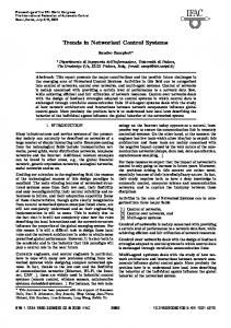
Figure 1: The structure of NCS.
actuator may be different from the data sent by the controller, which is called data drift. Data drift could cause negative impact on the system such as performance decline, even leading to instability. However, data drift in an NCS has not been taken into account in the literature above. In [22], Wang and Han first introduce a class of channel utilization-based switched controllers with controller-to-actuator data drift considered, and its results are established under the condition that data drift exists between controller and actuator, which may not be usable under the condition that data drift exists between sensor and controller. So, it is necessary to establish the results for NCS with sensor-to-controller data drift. Moreover, in [22], the guaranteed cost problem has not been considered, which motivates us to do this study. This paper aims at investigating the problem of guaranteed cost control for a class of continuous-time networked control systems with data drift. First of all, the sensor-tocontroller data drift is modeled as time-varying parameters. And a closed-loop model of networked control systems with time-varying parameters is established by lumping the network-induced delay and data-dropouts to a synthetically time-varying delay. Then, by using an appropriate Lyapunov functional, a guaranteed cost controller in terms of linear matrix inequality (LMI) is designed to cope with the effect of data drift and enhance the NCSs’ performance. The paper is organized in 5 sections including the Introduction. Section 2 presents problem formulations and modeling of NCS with data drift. Section 3 presents guaranteed cost controller design for NCS with data drift. There are some examples to illustrate the results in Section 4. Section 5 summarized this paper. Notations. 𝑅𝑛 denotes the 𝑛-dimensional Euclidean space. The superscript “𝑇” stands for matrix transposition. The notation 𝑋 > 0 means that the matrix 𝑋 is a real positive definite matrix. 𝐼 is the identity matrix of appropriate dimen𝑍 sions. [ 𝑋 ∗ 𝑌 ] denotes a symmetric matrix, where ∗ denotes the entries implied by symmetry.
2. Modeling of NCS with Data Drift
𝑢 (𝑡) = 𝐾𝑥 (𝑡 − 𝜏) , 𝑡 ∈ [𝑡𝑘 , 𝑡𝑘+1 ) , 𝑘 = 1, 2, . . . ,
(2)
where 𝐾 is the static state feedback gain matrix to be designed and 𝑡𝑘 is the sampling instant. Because the bandwidth is limited, data packet dropouts also happen in NCS. Considering that data packet dropouts may occur, the network is modeled as a switch. When the switch is located in position of 𝑆1 , the data packet containing 𝑥(𝑡𝑘 ) is transmitted, and the controller utilizes the updated data; but when it is located in position 𝑆2 , the data packet dropouts occur, and the controller uses the old data. Here only sensor-to-controller dropouts are considered. For a fixed sampling period ℎ, the dynamics of the switch can be expressed as follows: The NCS with no packet dropout at time 𝑡𝑘 : 𝑢 (𝑡) = 𝐾𝑥 (𝑡𝑘 − 𝜏) .
(3)
The NCS with one packet dropout at time 𝑡𝑘 : 𝑢 (𝑡) = 𝐾𝑥 (𝑡𝑘 − 𝜏 − ℎ) .. .
(4)
The NCS with 𝑑𝑘 ∈ 𝑍+ packet dropout at time 𝑡𝑘 : (2) can be rewritten as
Consider the linear control plant of NCS as follows: 𝑥̇ (𝑡) = 𝐴𝑥 (𝑡) + 𝐵𝑢 (𝑡) ,
where 𝑥(𝑡) ∈ 𝑅𝑛 and 𝑢(𝑡) ∈ 𝑅𝑚 represent state value and input and output separately; 𝐴 and 𝐵 are matrices with appropriate dimensions. The typical structure of NCS is shown in Figure 1. Transmission delays induced by the network are sensor-tocontroller delay 𝜏sc and controller-to-actuator delay 𝜏ca . In fact, these two delays can be lumped together as 𝜏 = 𝜏sc + 𝜏ca when the feedback controller is static. It assumes the state of the system is completely measurable. A piecewise static continuous feedback controller, which is realized by a zeroorder-hold (ZOH), is employed:
(1)
𝑢 (𝑡) = 𝐾𝑥 (𝑡𝑘 − 𝜏 − 𝑑𝑘 ℎ) .
(5)
Journal of Control Science and Engineering
3
When the control inputs are transmitted through network medium, data drift is unavoidable. In what follows, we take the sensor-to-controller data drift into account; it means the data received by controller is different from that sent by sensor. Considering the effect of data draft, we denote the ratio of data received by 𝑖th controller to the corresponding data sent by the 𝑖th controller by 𝐷𝑖 (𝑡) for any 𝑖 = 1, 2, . . . , 𝑛. And we define 𝐷(𝑡) = diag(𝐷1 (𝑡), 𝐷2 (𝑡), . . . , 𝐷𝑛 (𝑡)). Under the consideration of controller-to-actuator data drift, the control law in (5) is converted into 𝑢 (𝑡) = 𝐾𝐷 (𝑡) 𝑥 (𝑡𝑘 − 𝜏 − 𝑑𝑘 ℎ) .
(6)
Let 𝜂(𝑡) = 𝑡 − 𝑡𝑘 + 𝜏ca + 𝜏sc + 𝑑𝑘 ℎ; 𝑡 ∈ [𝑡𝑘 , 𝑡𝑘+1 ); (6) can be expressed as follows: 𝑢 (𝑡) = 𝐾𝐷 (𝑡) 𝑥 (𝑡 − 𝜂 (𝑡)) .
Remark 1. The networked control systems with sensor-tocontroller data drift are modeled as system (13). From (6), we know that if 𝐷(𝑡) = 𝐼, which means 𝐷𝑖 (𝑡) = 1 for any 𝑖 = 1, 2, . . . , 𝑛, sensor-to-controller data drift does not happen. In model (13), the uncertain matrix 𝐷(𝑡) denoting data drift is transformed to a bounded matrix 𝐹(𝑡) by introducing an upper bound and a lower bound for data drift. From (11), it is obvious that 𝐹𝑇 𝐹 = 𝐹2 ≤ 𝐼. Remark 2. Different from the models in literatures [18–21], the static feedback control gain matrix here is located between input matrix and the uncertain matrix induced by sensor-tocontroller data drift, which makes it more difficult to achieve the static control gain that can cope with the time-varying data drift.
(7)
3. Guaranteed Cost Controller Design of NCS with Data Drift
We assume it satisfies 𝜂𝑚 ≤ 𝜂 (𝑡) = 𝑡 − 𝑡𝑘 + 𝜏ca + 𝜏sc + 𝑑𝑘 ℎ ≤ 𝜂𝑀 𝑡 ∈ [𝑡𝑘 , 𝑡𝑘+1 ) .
(8)
The upper bound of variable 𝐷(𝑡) is defined as 𝐷𝑢 = diag(𝐷𝑢1 , 𝐷𝑢2 , . . . , 𝐷𝑢𝑛 ), 1 ≥ 𝐷𝑢𝑖 > 0, while the lower bound of variable 𝐷(𝑡) is defined as 𝐷𝑙 = diag(𝐷𝑙1 , 𝐷𝑙2 , . . . , 𝐷𝑙𝑛 ), 1 > 𝐷𝑙𝑖 ≥ 0. That is to say, 𝐷(𝑡) ∈ [𝐷𝑙 , 𝐷𝑢 ], which is timevarying. The average value of these two constant matrices can be obtained as
For system model (13) established in Section 2, the cost function is given as follows: ∞
𝐽 = ∫ 𝑥𝑇 (𝑡) 𝑆𝑥 (𝑡) 𝑑𝑡, 0
(14)
where 𝑆 is a symmetric positive definite matrix.
(9)
Definition 3. For system (13) and its cost function (14), if there exist a control gain matrix 𝐾 and a constant 𝐽0 , the cost function satisfies 𝐽 ≤ 𝐽0 . It is called matrix 𝐾 and is the guaranteed cost control gain of NCS.
Furthermore, the following time-varying matrix is introduced:
To analyze the stability of the system expediently, the following lemmas are introduced.
𝐹 (𝑡) = diag (𝑓1 (𝑡) , 𝑓2 (𝑡) , . . . , 𝑓𝑛 (𝑡)) ,
Lemma 4 (see [23]). For any matrices 𝑀, 𝑁, and 𝐹(𝑡) with 𝐹𝑇 𝐹 ≤ 𝐼 and any scalar 𝜀 > 0, the inequality holds as
𝐷0 = diag (𝐷01 , 𝐷02 , . . . , 𝐷0𝑛 ) , 𝐷0𝑖 =
𝑓𝑖 (𝑡) =
𝐷𝑢𝑖 + 𝐷𝑙𝑖 . 2
𝐷𝑖 (𝑡) − 𝐷0𝑖 . 𝐷0𝑖
(10)
𝑀𝐹 (𝑡) 𝑁 + 𝑁𝑇 𝐹𝑇 (𝑡) 𝑀𝑇 ≤ 𝜀𝑀𝑀𝑇 + 𝜀−1 𝑁𝑇 𝑁.
Obviously, we have −1 ≤
𝐷 (𝑡) − 𝐷0𝑖 𝐷𝑢𝑖 − 𝐷0𝑖 𝐷𝑙𝑖 − 𝐷0𝑖 ≤ 𝑓𝑖 (𝑡) = 𝑖 ≤ 𝐷0𝑖 𝐷0𝑖 𝐷0𝑖
(15)
(11)
The fundamental preliminary result is presented in the following theorem.
Based on (11), we have −𝐼𝑛×𝑛 ≤ 𝐹(𝑡) ≤ 𝐼𝑛×𝑛 . Based on (10), it knows 𝐷𝑖 = 𝐷0𝑖 (1 + 𝑓𝑖 (𝑡)), 𝑖 = 1, 2, . . . , 𝑛. Naturally, we have 𝐷 = 𝐷0 (𝐼 + 𝐹(𝑡)). Submitting this into (7), we have
Theorem 5. Given symmetric positive definite matrices 𝑆 and matrix 𝐾, if there exist a set of symmetric positive definite matrices 𝑄1 , 𝑄2 , 𝑅1 , and 𝑅2 and matrix 𝑃 > 0, as well as matrices 𝑀1 , 𝑀2 , 𝑀3 , 𝑀4 , and 𝑀5 and a constant 𝜀 > 0, satisfying the matrix inequality as
=
𝐷𝑢𝑖 − 𝐷𝑙𝑖 ≤ 1. 𝐷𝑢𝑖 + 𝐷𝑙𝑖
𝑢 (𝑡) = 𝐾𝐷0 (𝐼 + 𝐹 (𝑡)) 𝑥 (𝑡 − 𝜂 (𝑡)) .
(12)
Submitting (12) into (1), the following follows: 𝑥̇ (𝑡) = 𝐴𝑥 (𝑡) + 𝐵𝐾𝐷0 (𝐼 + 𝐹 (𝑡)) 𝑥 (𝑡 − 𝜂 (𝑡)) .
(13)
Π Ξ 𝐼̂ ] [ [∗ 𝜀−1 𝐼 0 ] < 0, ] [ [∗ ∗ 𝜀𝐼]
(16)
4
Journal of Control Science and Engineering
where Π [ [ [ [ [ [ [ =[ [ [ [ [ [ [
𝑄1 + 𝑀1 𝐴 + 𝐴𝑇 𝑀1 𝑇 − 𝑅1 + 𝑆
𝐴𝑇 𝑀3 𝑇 + 𝑅1
𝐴𝑇 𝑀4 𝑇
∗
1 𝑄2 − 𝑄1 − 𝑅1 − 𝑅 𝜂𝑀 − 𝜂𝑚 2
∗
∗
1 𝑅 𝜂𝑀 − 𝜂𝑚 2 1 −𝑄2 − 𝑅 𝜂𝑀 − 𝜂𝑚 2
∗
∗
∗
𝑀2 𝐵𝐾𝐷0 + (𝐵𝐾𝐷0 ) 𝑀2 𝑇
∗
∗
∗
∗
[
𝑀1 𝐵𝐾𝐷0 + 𝐴𝑇 𝑀2 𝑇 𝑀3 𝐵𝐾𝐷0 𝑀4 𝐵𝐾𝐷0 𝑇
𝐴𝑇 𝑀5 𝑇 − 𝑀1 + 𝑃
] ] ] −𝑀3 ] ] ] ] ], −𝑀4 ] ] ] 𝑇 𝑇 (𝐵𝐾𝐷0 ) 𝑀5 − 𝑀2 ] ] ] 𝑇 Ω − 𝑀5 + 𝑀5 ]
2 𝑅1 + (𝜂𝑀 − 𝜂𝑚 ) 𝑅2 , Ω = 𝜂𝑚
(17)
𝑀1 𝐵𝐾𝐷0 [ ] [𝑀3 𝐵𝐾𝐷0 ] [ ] [ ] Ξ = [𝑀4 𝐵𝐾𝐷0 ] , [ ] [𝑀 𝐵𝐾𝐷 ] [ 2 0] [𝑀5 𝐵𝐾𝐷0 ] 0 [ ] [0] [ ] [ ] 𝐼̂ = [0] , [ ] [𝐼] [ ] [0]
then system (13) is asymptotically stable. And the cost function 𝐽 satisfies 𝐽 ≤ 𝑥𝑇 (0) 𝑃𝑥 (0) + ∫
0
−𝜂𝑚
+∫
−𝜂𝑚
𝑡
𝑡−𝜂𝑚
𝑡−𝜂𝑚
𝑥𝑇 (𝛼) 𝑄1 𝑥 (𝛼) 𝑑𝛼
+∫
𝑡−𝜂𝑀
𝑡
∫ 𝑥̇𝑇 (𝛿) 𝑅1 𝑥̇ (𝛿) 𝑑𝜃 𝑑𝛿 𝜃
𝑡
∫ 𝑥̇𝑇 (𝜔) 𝑅2 𝑥̇ (𝜔) 𝑑𝜏 𝑑𝜔 , 𝜏
(20)
𝑥𝑇 (𝛼) 𝑄2 𝑥 (𝛼) 𝑑𝛼
−𝜂𝑀
0
𝑡
+ 𝜂𝑚 ∫
−𝜂𝑚
+∫
𝑉3 (𝑡) = 𝜂𝑚 ∫
−𝜂𝑚
−𝜂𝑀
(18) 𝑇
∫ 𝑥̇ (𝛿) 𝑅1 𝑥̇ (𝛿) 𝑑𝜃 𝑑𝛿 𝜃
with 𝑃 > 0, 𝑄1 > 0, 𝑄2 > 0, 𝑅1 > 0, and 𝑅2 > 0. Calculating the derivative of Lyapunov-Krasovskii function and based on (13), it follows that
𝑡
∫ 𝑥̇𝑇 (𝜔) 𝑅2 𝑥̇ (𝜔) 𝑑𝜏 𝑑𝜔 .
𝑉̇ (𝑡) = 2𝑥𝑇 (𝑡) 𝑃𝑥̇ (𝑡) + 𝑥𝑇 (𝑡) 𝑄1 𝑥 (𝑡) + 𝑥𝑇 (𝑡 − 𝜂𝑚 )
𝜏
Proof. First of all, we consider the Lyapunov-Krasovskii function as follows: 𝑉 (𝑡) = 𝑉1 (𝑡) + 𝑉2 (𝑡) + 𝑉3 (𝑡) ,
(19)
⋅ (𝑄2 − 𝑄1 ) 𝑥 (𝑡 − 𝜂𝑚 ) − 𝑥𝑇 (𝑡 − 𝜂𝑀) 𝑄2 𝑥 (𝑡 − 𝜂𝑀) 2 + 𝑥̇𝑇 (𝑡) [𝜂𝑚 𝑅1 + (𝜂𝑀 − 𝜂𝑚 ) 𝑅2 ] 𝑥̇ (𝑡)
− 𝜂𝑚 ∫
where
𝑡
𝑡−𝜂𝑚
𝑇
𝑉1 (𝑡) = 𝑥 (𝑡) 𝑃𝑥 (𝑡) , 𝑡
𝑉2 (𝑡) = ∫
𝑡−𝜂𝑚
+∫
𝑥𝑇 (𝛼) 𝑄1 𝑥 (𝛼) 𝑑𝛼
𝑡−𝜂𝑚
𝑡−𝜂𝑀
𝑥𝑇 (𝛼) 𝑄2 𝑥 (𝛼) 𝑑𝛼,
𝑡−𝜂𝑚
+∫
𝑡−𝜂𝑀
𝑥̇𝑇 (𝜃) 𝑅1 𝑥̇ (𝜃) 𝑑𝜃
𝑥̇𝑇 (𝑠) 𝑅2 𝑥̇ (𝑠) 𝑑𝑠 + 2 [𝑥𝑇 (𝑡) 𝑀1
+ 𝑥𝑇 (𝑡 − 𝜂 (𝑡)) 𝑀2 + 𝑥𝑇 (𝑡 − 𝜂𝑚 ) 𝑀3 + 𝑥𝑇 (𝑡 − 𝜂𝑀) 𝑀4 + 𝑥̇𝑇 (𝑠) 𝑀5 ] .
(21)
Journal of Control Science and Engineering
5
Based on Jensen’s inequality, also used in [19], we have − 𝜂𝑚 ∫
𝑡
𝑡−𝜂𝑚
𝑥̇𝑇 (𝑠) 𝑅1 𝑥̇ (𝑠) 𝑑𝑠 ≤ [𝑥𝑇 (𝑡) , 𝑥𝑇 (𝑡 − 𝜂𝑚 )]
−𝑅1 𝑅1
⋅[ −∫
𝑅1 −𝑅1
𝑡−𝜂𝑚
𝑡−𝜂𝑀
[ [ [ [ [ [ [ [ [ [ [
∗
[
𝑥 (𝑡)
Applying Lemma 4 and Schur complement to inequality (16), we have
𝐴𝑇 𝑀3 𝑇 + 𝑅1 1 𝑅 𝑄2 − 𝑄1 − 𝑅1 − 𝜂𝑀 − 𝜂𝑚 2
∗
∗
∗
∗
∗
∗
𝐴𝑇 𝑀4 𝑇 𝑀1 Θ + 𝐴𝑇 𝑀2 𝑇 𝐴𝑇 𝑀5 𝑇 − 𝑀1 + 𝑃 ] 1 ] 𝑅2 𝑀3 Θ −𝑀3 ] ] 𝜂𝑀 − 𝜂𝑚 ] ] < 0, 1 ] −𝑄2 − 𝑅2 𝑀4 Θ −𝑀4 ] 𝜂𝑀 − 𝜂𝑚 ] ] 𝑇 𝑇 ∗ 𝑀2 Θ Θ 𝑀4 − 𝑀2 ] ∗
where Θ = 𝐵𝐾𝐷0 (𝐼 + 𝐹(𝑡)). From (21)–(23), based on Schur complement, it follows that 𝑉̇ (𝑡) ≤ −𝑥𝑇 (𝑡) 𝑆𝑥 (𝑡) ≤ 0.
(24)
Therefore, system (13) is asymptotically stable and there exists lim𝑡 → ∞ 𝑥(𝑡) = 0. And through the integral operation, we have ∞
∫ 𝑉̇ (𝑡) 𝑑𝑡 = 𝑉 (∞) − 𝑉 (0) = −𝑉 (0) 0
𝑅2
(22)
𝑥̇𝑇 (𝑠) 𝑅2 𝑥̇ (𝑠) 𝑑𝑠
𝑄1 + 𝑀1 𝐴 − 𝑅1 + 𝑆
𝑥 (𝑡 − 𝜂𝑚 ) ][ ]. −𝑅2 𝑥 (𝑡 − 𝜂𝑀)
−𝑅2 𝑅2
⋅[
], 𝑥 (𝑡 − 𝜂𝑚 )
][
1 [𝑥𝑇 (𝑡 − 𝜂𝑚 ) , 𝑥𝑇 (𝑡 − 𝜂𝑀)] 𝜂𝑀 − 𝜂𝑚
≤
∞
≤ − ∫ 𝑥𝑇 (𝑡) 𝑆𝑥 (𝑡) 𝑑𝑡 = −𝐽.
∗
]
Remark 6. The condition of stability is expressed with matrix inequality (16). It is worthy to point out that inequality (16) is not linear with respect to the gain matrix of the controller, so it is needed to be reformulated into LMIs via a change of variables. Theorem 7. Given a set of constants 𝜉𝑖 (𝑖 = 1, 2, 3, 4), 𝜂𝑚 , and 𝜂𝑀, if there exist a set of symmetric positive definite matrices ̃1 , 𝑄 ̃2 , 𝑅 ̃1 , 𝑅 ̃ 2 , and 𝑆̃ and a constant 𝜀 > 0, as well as matrices 𝑄 ̃ 𝑃 > 0 and 𝑋 > 0 and matrix 𝑍 satisfying LMI as
(25)
̃ Ξ ̃ 𝜀−1 𝐼̂ Π [ ] −1 [∗ 𝜀 𝐼 0 ] < 0, −1 [∗ ∗ 𝜀 𝐼]
0
So the inequality 𝐽 ≤ 𝑉(0) holds; submitting 𝑡 = 0 to Lyapunov-Krasovskii function (19), the inequality (18) can be obtained. This completes the proof.
Ω − 𝑀5
(23)
(26)
where
̃ Π ̃ 1 + 𝑆̃ ̃1 ̃1 + 𝜉1 𝐴𝑋𝑇 + 𝜉1 𝑋𝐴𝑇 − 𝑅 𝜉3 𝑋𝐴𝑇 + 𝑅 𝜉4 𝑋𝐴𝑇 𝜉1 𝐵𝑍 + 𝜉2 𝑋𝐴𝑇 𝑋𝐴𝑇 − 𝜉1 𝑋𝑇 + 𝑃̃ 𝑄 [ ] 1 1 [ ] ̃2 ̃2 ̃1 − 𝑅 ̃1 − ̃2 − 𝑄 [ ] 𝑅 𝑅 𝜉3 𝐵𝑍 −𝜉3 𝑋𝑇 ∗ 𝑄 [ ] 𝜂𝑀 − 𝜂𝑚 𝜂𝑀 − 𝜂𝑚 [ ] [ ] 1 =[ ], 𝑇 ̃ ̃ 𝑅 ∗ ∗ − 𝑄 − 𝜉 𝐵𝑍 −𝜉 𝑋 [ ] 2 2 4 4 𝜂𝑀 − 𝜂𝑚 [ ] [ ] 𝑇 𝑇 𝑇 [ ] ∗ ∗ ∗ 𝜉 𝐵𝑍 + 𝜉 − 𝜉 𝑋 (𝐵𝑍) 2 2 (𝐵𝑍) 2 [ ] [
∗
̃ 1 + (𝜂𝑀 − 𝜂𝑚 ) 𝑅 ̃2 , ̃ = 𝜂𝑚 2 𝑅 Ω 𝜉1 𝐵𝑍 [𝜉 𝐵𝑍] [ 3 ] ] ̃=[ Ξ [𝜉4 𝐵𝑍] , ] [ [𝜉2 𝐵𝑍] [ 𝐵𝑍 ]
∗
∗
∗
̃ − 𝑋 − 𝑋𝑇 ] Ω
(27)
6
Journal of Control Science and Engineering 2
then system (13) is asymptotically stable with the guaranteed cost controller 𝐾 = 𝑍𝑋−𝑇 𝐷0−1 , where matrix 𝐷0 is determined by the average value of data drift, and the cost function 𝐽 satisfies −1 ̃
𝑇
−𝑇
0
̃1 𝑋−𝑇 𝑥 (𝛼) 𝑑𝛼 𝑥𝑇 (𝛼) 𝑋−1 𝑄
−𝜂𝑚
+∫
−𝜂𝑚
−𝜂𝑀
+ 𝜂𝑚 ∫ −𝜂𝑚
−𝜂𝑀
1.2 1 0.8 0.6
𝑥
̃2 𝑋−𝑇 𝑥 (𝛼) 𝑑𝛼 (𝛼) 𝑋−1 𝑄
𝑇
0
0.4
(28)
0.2
𝑡
−𝜂𝑚
+∫
1.4
̃ 1 𝑋−𝑇 𝑥̇ (𝛿) 𝑑𝜃 𝑑𝛿 ∫ 𝑥̇𝑇 (𝛿) 𝑋−1 𝑅
0
𝜃
𝑡
̃ 2 𝑋−𝑇 𝑥̇ (𝜔) 𝑑𝜏 𝑑𝜔 . ∫ 𝑥̇𝑇 (𝜔) 𝑋−1 𝑅
1
2
3
4
5 6 Time (s)
7
8
9
10
𝜏
Proof. This Theorem is obtained through a suitable transformation on the basis of inequality (16) in Theorem 5. Firstly, we define 𝑀𝑖 = 𝜉𝑖 𝑀5 (𝑖 = 1, 3, 4, 5) in (16). Obviously, (16) implies that 𝑀5 > 0, so 𝑀5 is nonsingular. Then, pre- and post-multiplying both sides of inequality (16) ̃ 𝐼, 𝜀−1 𝐼) and its transpose, and introducing new with diag(𝑋, ̃ 𝑋𝑃𝑋𝑇 = 𝑃; ̃ 𝑋𝑅𝑗 𝑋𝑇 = 𝑅 ̃ 𝑗 , 𝑋𝑄𝑗 𝑋𝑇 = 𝑄 ̃𝑗 variables 𝑋𝑆𝑋𝑇 = 𝑆;
(𝑗 = 1, 2); 𝐾𝐷0 𝑋𝑇 = 𝑍, it follows inquality (26), where ̃ = diag(𝑋, 𝑋, 𝑋, 𝑋, 𝑋) and 𝑋 = 𝑀5 −1 . From the definition 𝑋 of 𝐷0 in (9), we know 𝐷0 is invertible, so 𝐾 can be obtained by calculating 𝐾 = 𝑍𝑋−𝑇 𝐷0−1 . And it is easy to see that (26) and (28), respectively, imply (16) and (18). Therefore, from Theorem 5, we can complete the proof.
2
1.8 1.6 1.4 1.2 1 0.8 0.6 0.4 0.2 0
4. Simulations 0 0
1.02 ] [−0.1] ] 𝑢 (𝑡) . ] 𝑥 (𝑡) + [
0 −0.801]
(29)
3
4
5 6 Time (s)
7
8
9
10
1.6
For this simulation, we synthetically consider a time-varying delay by lumping the network-induced delay and packet dropouts together with upper bound 𝜂𝑀 = 0.61 s and lower bound 𝜂𝑚 = 0.12 s; namely, 0.12 ≤ 𝜂(𝑡) ≤ 0.61. Here timevarying sensor-to-controller data drift with the average value 𝐷0 = diag(0.6, 0.71, 0.6) is also considered, which is shown in Figure 2. We choose the parameters 𝜉1 = 0.0002, 𝜉2 = 11110.0001, 𝜉3 = 1.005, and 𝜉4 = −0.001. By taking advantage of LMI toolbox and submitting these parameters above into inequality (26), we can obtain the guaranteed cost control gain
with 𝜀 = 3.7545 × 10¹⁶ .
2
1.8
[−0.2]
𝐾 = 𝑍𝑋−𝑇 𝐷0−1 = [−7.5329 −0.3563 0.4067]
1
2
1.4 Data drift D3 (t)
3 1 [−1 −2 𝑥̇ (𝑡) = [
0
(b) Data drift in the second channel from sensor to controller
Example 8. Consider the linear system as follows:
[0
0
(a) Data drift in the first channel from sensor to controller
Data drift D2 (t)
+∫
1.6 Data drift D1 (t)
𝐽 ≤ 𝑥 (0) 𝑋 𝑃𝑋 𝑥 (0)
1.8
1.2 1 0.8 0.6 0.4 0.2 0
0
1
2
3
4
5 6 Time (s)
7
8
9
(c) Data drift in the third channel from sensor to controller
(30) Figure 2: The time-varying data drift.
10
Journal of Control Science and Engineering
7
0.8
×108 2
0.7
1.5
0.6
1 0.5 0
0.4
State x
State x
0.5
0.3
−0.5 −1 −1.5
0.2
−2
0.1
−2.5
0.0
−3
−0.1
0
1
2
3
4
5 6 Time (s)
7
8
9
10
x1 x2 x3
0
1
2
3
4
5 6 Time (s)
7
8
9
10
x1 x2 x3
Figure 5: The state response curves of NCS with data drift.
Figure 3: The state response curves of NCS with data drift.
To better illustrate the effectiveness of the method proposed in this paper, the following example is discussed. 0.005
Example 9. Consider the linear model of NCS as follows
0
−0.5 1.36 0 0.52 [ ] 0 0.21] [−0.61 1.1 [ ] 𝑥 (𝑡) 𝑥̇ (𝑡) = [ ] [ 0.16 0.29 −1.42 0 ]
Control input
−0.005 −0.01
[ 0 1.37
−0.015
−0.12 0.26]
(31)
[ ] [ −1.1 ] [ ] 𝑢 (𝑡) . +[ ] [ 1.55 ]
−0.02 −0.025
1
[−0.73] 0
1
2
3
4
5 6 Time (s)
7
8
9
10
Figure 4: The control input of NCS with data drift.
The initial state of system is assumed 𝑥(0) = 𝑇 0.3 0.8] [0.6 , through the state response of NCS with the effect of data drift shown in Figure 3 and corresponding control input shown in Figure 4, we know all states of system get steady at 7.3 s. In addition, we apply the method proposed by Luck [10] into the same problem. And the design of controller fails with 𝐾 = [0.4285 −1.0243 0 0.4243], the response of system state is shown as Figure 5. Thus, it sufficiently demonstrates the effectiveness and feasibility of the guaranteed cost method proposed in this paper.
For this simulation, we set the time-varying delay with upper bound 𝜂𝑀 = 0.15 s and lower bound 𝜂𝑚 = 0.09 s. And time-varying sensor-to-controller data drift with the average value 𝐷0 = diag(0.52, 0.61, 0.36, 0.65) is also considered. By taking advantage of LMI toolbox and submitting these parameters above into inequality (26), we can obtain the guaranteed cost control gain 𝐾 = 𝑍𝑋−𝑇 𝐷0−1 = [−1.8322 −1.5264 −0.3754 −2.5736]. The initial state of 𝑇 system is assumed 𝑥(0) = [1.2 0.47 0.12 −1.13] ; through the state response of NCS with the effect of data drift shown in Figure 6, we know all states of system get steady at 60 s. The guaranteed cost controller designed in this paper is able to make the NCS asymptotically stable even if affected by data drift. It sufficiently proves the effectiveness and feasibility of the method proposed in this paper.
8
Journal of Control Science and Engineering 1.5
References
1
State x
0.5 0 −0.5 −1 −1.5
0
10
20
30
x1 x2
40
50 60 Time (s)
70
80
90
100
x3 x4
Figure 6: The state response curves of NCS with data drift.
5. Conclusions The guaranteed cost control problem of a class of continuoustime networked control systems with data drift is investigated. With sensor-to-controller data drift considered, networked control system is modeled as a closed-loop system with time-varying parameters by lumping the networkinduced delay and data-dropouts to a synthetically timevarying delay together. Moreover, by selecting an appropriate Lyapunov function, the guaranteed cost controller in terms of linear matrix inequality (LMI) is designed to cope with the effect of data drift and enhance the NCS’s performance. And a simulation is given to prove the effectiveness and feasibility of the method. The convexity substitutions used in Theorem 7 (𝑀𝑖 = 𝜉𝑖 𝑀5 (𝑖 = 1, 3, 4, 5)) may, in general, lead to significantly conservative results. Our next research task will be choosing more reasonable values of parameters 𝜉𝑖 (𝑖 = 1, 2, 3, 4) to reduce the conservatism further.
Conflict of Interests The authors declare that there is no conflict of interests regarding the publication of this paper.
Acknowledgments This work was partly supported by National Nature Science Foundation of China (61164014, 51375323, and 61563022), Major Program of Natural Science Foundation of Jiangxi Province, China (20152ACB20009), and Qing Lan Project of Jiangsu Province, China.
[1] J. Liu and D. Yue, “Event-triggering in networked systems with probabilistic sensor and actuator faults,” Information Sciences, vol. 240, pp. 145–160, 2013. [2] M. Jungers, E. B. Castelan, V. M. Moraes, and U. F. Moreno, “A dynamic output feedback controller for NCS based on delay estimates,” Automatica, vol. 49, no. 3, pp. 788–792, 2013. [3] Y. Xia, W. Xie, B. Liu, and X. Wang, “Data-driven predictive control for networked control systems,” Information Sciences, vol. 235, pp. 45–54, 2013. [4] Y. Zhang and J. Jiang, “Bibliographical review on reconfigurable fault-tolerant control systems,” Annual Reviews in Control, vol. 32, no. 2, pp. 229–252, 2008. [5] V. B. Kolmanovskii and J.-P. Richard, “Stability of some linear systems with delays,” IEEE Transactions on Automatic Control, vol. 44, no. 5, pp. 984–989, 1999. [6] C. Peng and T. C. Yang, “Event-triggered communication and 𝐻∞ control co-design for networked control systems,” Automatica, vol. 49, no. 5, pp. 1326–1332, 2013. [7] H. Song, L. Yu, and W.-A. Zhang, “Networked 𝐻∞ filtering for linear discrete-time systems,” Information Sciences, vol. 181, no. 3, pp. 686–696, 2011. [8] A. Ray and Y. Halevi, “Integrated communication and control systems: part II—design considerations,” Journal of Dynamic Systems, Measurement and Control, vol. 110, no. 4, pp. 374–381, 1988. ¨ uner, “Closed-loop control of systems over ¨ Ozg¨ [9] H. Chan and U. a communications network with queues,” International Journal of Control, vol. 62, no. 3, pp. 493–510, 1995. [10] R. Luck and A. Ray, “An observer-based compensator for distributed delays,” Automatica, vol. 26, no. 5, pp. 903–908, 1990. [11] J. Nilsson, Real-time control systems with delays [Ph.D. thesis], Lund Institute of Technology, 1998. [12] J. Xiong and J. Lam, “Stabilization of networked control systems with a logic ZOH,” IEEE Transactions on Automatic Control, vol. 54, no. 2, pp. 358–363, 2009. [13] K. Liu and E. Fridman, “Networked-based stabilization via discontinuous Lyapunov functionals,” International Journal of Robust and Nonlinear Control, vol. 22, no. 4, pp. 420–436, 2012. [14] X. Meng, J. Lam, and H. Gao, “Network-based H ∞ control for stochastic systems,” International Journal of Robust and Nonlinear Control, vol. 19, no. 3, pp. 295–312, 2009. [15] J. Li, Q. Zhang, H. Yu, and M. Cai, “Real-time guaranteed cost control of MIMO networked control systems with packet disordering,” Journal of Process Control, vol. 21, no. 6, pp. 967– 975, 2011. [16] T. H. Lee, J. H. Park, D. H. Ji, O. M. Kwon, and S. M. Lee, “Guaranteed cost synchronization of a complex dynamical network via dynamic feedback control,” Applied Mathematics and Computation, vol. 218, no. 11, pp. 6469–6481, 2012. [17] X. Fang and J. Wang, “Stochastic observer-based guaranteed cost control for networked control systems with packet dropouts,” IET Control Theory & Applications, vol. 2, no. 11, pp. 980–989, 2008. [18] R. Wang, G.-P. Liu, W. Wang, D. Rees, and Y. B. Zhao, “Guaranteed cost control for networked control systems based on an improved predictive control method,” IEEE Transactions on Control Systems Technology, vol. 18, no. 5, pp. 1226–1232, 2010. [19] J.-S. Xie, B.-Q. Fan, J. Yang et al., “Guaranteed cost controller design of networked control systems with state delay,” Acta Automatica Sinica, vol. 33, no. 2, pp. 170–174, 2007.
Journal of Control Science and Engineering [20] L. Xie, H. Fang, and Y. Zheng, “Guaranteed cost control for networked control systems,” Journal of Control Theory and Applications, vol. 2, no. 2, pp. 143–148, 2004 (Chinese). [21] X. Li and X.-B. Wu, “Guaranteed cost fault-tolerant controller design of networked control systems under variable-period sampling,” Information Technology Journal, vol. 8, no. 4, pp. 537– 543, 2009. [22] Y.-L. Wang and Q.-L. Han, “Modelling and controller design for discrete-time networked control systems with limited channels and data drift,” Information Sciences, vol. 269, pp. 332–348, 2014. [23] G. Garcia, J. Bernussou, and D. Arzelier, “Robust stabilization of discrete-time linear systems with norm-bounded time-varying uncertainty,” Systems and Control Letters, vol. 22, no. 5, pp. 327– 339, 1994.
9
International Journal of
Rotating Machinery
Engineering Journal of
Hindawi Publishing Corporation http://www.hindawi.com
Volume 2014
The Scientific World Journal Hindawi Publishing Corporation http://www.hindawi.com
Volume 2014
International Journal of
Distributed Sensor Networks
Journal of
Sensors Hindawi Publishing Corporation http://www.hindawi.com
Volume 2014
Hindawi Publishing Corporation http://www.hindawi.com
Volume 2014
Hindawi Publishing Corporation http://www.hindawi.com
Volume 2014
Journal of
Control Science and Engineering
Advances in
Civil Engineering Hindawi Publishing Corporation http://www.hindawi.com
Hindawi Publishing Corporation http://www.hindawi.com
Volume 2014
Volume 2014
Submit your manuscripts at http://www.hindawi.com Journal of
Journal of
Electrical and Computer Engineering
Robotics Hindawi Publishing Corporation http://www.hindawi.com
Hindawi Publishing Corporation http://www.hindawi.com
Volume 2014
Volume 2014
VLSI Design Advances in OptoElectronics
International Journal of
Navigation and Observation Hindawi Publishing Corporation http://www.hindawi.com
Volume 2014
Hindawi Publishing Corporation http://www.hindawi.com
Hindawi Publishing Corporation http://www.hindawi.com
Chemical Engineering Hindawi Publishing Corporation http://www.hindawi.com
Volume 2014
Volume 2014
Active and Passive Electronic Components
Antennas and Propagation Hindawi Publishing Corporation http://www.hindawi.com
Aerospace Engineering
Hindawi Publishing Corporation http://www.hindawi.com
Volume 2014
Hindawi Publishing Corporation http://www.hindawi.com
Volume 2014
Volume 2014
International Journal of
International Journal of
International Journal of
Modelling & Simulation in Engineering
Volume 2014
Hindawi Publishing Corporation http://www.hindawi.com
Volume 2014
Shock and Vibration Hindawi Publishing Corporation http://www.hindawi.com
Volume 2014
Advances in
Acoustics and Vibration Hindawi Publishing Corporation http://www.hindawi.com
Volume 2014