___________________________ The Stochastic Eulerian Tour Problem Srimathy Mohan Michel Gendreau Jean-Marc Rousseau
October 2007
CIRRELT-2007-45
The Stochastic Eulerian Tour Problem Srimathy Mohan1, Michel Gendreau2,3,*, Jean-Marc Rousseau2 1.
School of Global Management and Leadership, MC 2451, Arizona State University, P.O. Box 37100, Phoenix, AZ 85069-7100, USA
2.
Interuniversity Research Centre on Enterprise Networks, Logistics and Transportation (CIRRELT), Université de Montréal, P.O. Box 6128, Station Centre-ville, Montréal, Canada H3C 3J7
3.
Department of Computer Science and Operations Research, Université de Montréal, P.O. Box 6128, Station Centre-ville, Montréal, Canada H3C 3J7
Abstract. This paper defines the Stochastic Eulerian Tour Problem (SETP) and investigates several characteristics of this problem. Given an undirected Eulerian graph G = (V , E ) , a subset R ( R = n ) of the edges in E that require service, and a probability distribution for the number of edges in R that have to be visited in any given instance of the graph, the SETP seeks an a priori Eulerian tour of minimum expected length. We derive a closed form expression for the expected length of a given Eulerian tour when the number of required edges that have to be visited follows a binomial distribution. We also show that the SETP is NP-hard, even though the deterministic counter part is solvable in polynomial time. We derive further properties and a worst case ratio of the deviation of the expected length of a random Eulerian tour from the expected length of the optimal tour. Finally, we present some of the desirable properties in a good a priori tour using illustrative examples. Keywords. Arc routing, Eulerian tour problem, stochastic demand. Acknowledgements. Financial support for this work was provided by the Natural Sciences and Engineering Research Council of Canada (NSERC) and by the Fonds FCAR (renamed Fonds québécois de la recherche sur la nature et les technologies, FQRNT). This support is gratefully acknowledged. Results and views expressed in this publication are the sole responsibility of the authors and do not necessarily reflect those of CIRRELT. Les résultats et opinions contenus dans cette publication ne reflètent pas nécessairement la position du CIRRELT et n'engagent pas sa responsabilité.
_____________________________ * Corresponding author:
[email protected]
This document is also published as Publication #1308 by the Department of Computer Science and Operations Research of the Université de Montréal. Dépôt légal – Bibliothèque nationale du Québec, Bibliothèque nationale du Canada, 2007 © Copyright Mohan, Gendreau, Rousseau and CIRRELT, 2007
The Stochastic Eulerian Tour Problem
1.
Introduction
One of the most common problems in routing is the design of routes for people or vehicles delivering service. Such routing problems are of two types -- node routing and arc routing problems, depending on whether the service request is at a node or on an arc/edge. The underlying problem for most arc routing problems is determining a giant tour that starts and ends at a designated depot, and traverses all edges requiring service at least once. This is the deterministic Eulerian Tour Problem (ETP). A connected graph is Eulerian if there exists a closed walk in the graph containing each edge exactly once. If the given graph is not Eulerian, the first step is to add a least cost set of arcs or edges to the graph to make it Eulerian. This is called the least cost augmentation problem. Edmonds and Johnson (1973) show that this problem can be solved in polynomial time for the undirected Chinese Postman Problem (CPP) using an adaptation of Edmond’s blossom algorithm. While the least cost augmentation problem for directed graphs is also solvable in polynomial time, it is NP-hard when the underlying graph contains both arcs and edges. In this case, heuristics are used to make the graph Eulerian. Given an Eulerian graph, an Eulerina tour can be determined in polynomial time. Edmonds and Johnson (1973) have described three different algorithms for the ETP on an undirected graph. These are the end-pairing algorithm, the next-node algorithm, and the maze-search algorithm. The ETP is well solved for directed and mixed graphs also. van Aardenne-Ehrenfest and de Bruijn describe the spanning arborescence algorithm for the ETP on directed graphs. For mixed graphs, one usually assigns directions to the undirected edges to transform the mixed graph into a symmetric graph, and then completely orient the remaining undirected edges so that the indegree equals to the outdegree for all vertices of the graph. The spanning arborescence algorithm can then be used to determine the Eulerian tour for this graph. In this paper, we assume that we have solved the least cost augmentation problem and are given an undirected Eulerian graph G = (V , E ) in which the set R (R ⊆ E ) represents the set of edges that require service. It is important to note that there may be more than one Eulerian tour for a given graph. However, all these tours have the same cost and hence there is no optimization involved in the ETP. But
CIRRELT-2007-45
1
The Stochastic Eulerian Tour Problem
there exist quite a few situations in practice, when not all the edges that require service need to be visited everyday. In such cases, the number of edges that require a visit on any given day is a random variable. For example, consider a postal carrier who has to deliver mail to n different streets. The postal company wishes to minimize the total walking distance for the carrier.
When the carrier has to visit all the n
streets every day, any Eulerian tour would suffice, since all the Eulerian tours are of equal length. But in reality, based on the realization of demand, the carrier might have to visit only a subset of the streets requiring service on any particular day. Consider the following alternative in that situation: the postal carrier follows the predetermined tour as long as he has to visit the next street on the tour to provide service. If at any point on the tour, the postal carrier does not have to visit a street, he skips that street, and takes the shortest path to the next street on the tour that requires a visit. With this alternative, the ETP takes on a different dimension. The different possible Eulerian tours of a graph yield themselves better to skipping certain edges of the graph. We use the example in Figure 1 to illustrate this. All edges of the underlying undirected graph have a length of 1 and the edges represented by solid lines require service. Node O represents the depot. The dotted lines represent the edges that are only traversed and not serviced. Tours 1 and 2 are two different Eulerian tours for the same graph. The numbers on the edges of the two tours represent the order in which one visits the edges in these tours.
TOUR 2
TOUR 1 1 3
16
4
1 5
2
14
10
11
12
9
6
5
7
3
12
6
15 13
16
7
2
4
15 8
11
13 10
14
8
9
Figure 1. Two different tours for a 3x3 undirected graph On a particular day, let us assume that edges A, B, C, and D require service. This translates to edges 2, 6, 10, and 14 on tour 1 and edges 4, 5, 12, and 13 on tour 2. If we start at the depot, visit the
CIRRELT-2007-45
2
The Stochastic Eulerian Tour Problem
edges in the same order that they appear in the respective tours and return to the depot, tour 1 results in a total length of 10 (Depot-1-2-7-6-11-10-15-14-15-16-Depot), while tour 2 results in a length of 12 (Depot-1-2-3-4-5-6-15-12-13-10-11-16-Depot). Thus, tour 1 is better for this instance. On the other hand, if edges A, C, E and F require service, tour 2 which has a length of 6 (Depot-1-2-3-4-5-1-Depot) is better than tour 1 which has a length of 8 (Depot-1-2-3-4-5-6-3-1-Depot).
Hence, under such
circumstances, the objective is to determine not just any Eulerian tour, but a particular tour (if more than one tour exists for the given graph) which has the shortest tour length “on an average”. This motivates the investigation of the Stochastic Eulerian Tour Problem (SETP) which we define below.
(
)
We are given an undirected Eulerian graph G = (V , E ) , a set R R ⊆ E , R = n of edges that
(
require service (We shall call them “white” edges following the notation in [6].), and a distance d vi , v j
)
between every pair of directly connected nodes vi and v j . On any instance of the problem, only a subset of the n white edges is present, and hence, requires a visit. The number of present edges follows a specified probability distribution. The objective is to determine an a priori Eulerian tour that visits all the n edges and minimizes the expected length of the tour. On any given instance, one visits and services the present edges in the same order as in the a priori tour, while skipping the ones that are absent. Our investigation of the SETP has also been motivated by a real-world problem. In the UK postal system, the postal carriers usually deliver mail a second time in the afternoon. During the first mail delivery, the carriers have to visit all the streets almost always, whereas the second mail delivery is typically very light. Only a small subset of the streets requires service during the afternoon delivery. While any Eulerian tour would be sufficient for the first mail delivery, it is definitely advantageous to determine a tour that minimizes the total length in an expected sense for the second mail delivery. It is important to note that even though the ETP is well solved, it is not feasible to determine a new tour for each day, since following a new tour every day would decrease the operating efficiency of the postal carrier considerably. In certain applications, like Canada Post, the mail carrier collects the mail to be delivered at various points along the route from relay boxes. On any given day, the present edges are
CIRRELT-2007-45
3
The Stochastic Eulerian Tour Problem
known only after the carrier starts his route and thus, it is not possible for the carrier to determine a new route at the start of each day. In such situations, it is certainly efficient to let the mail carrier follow the same route every day, while allowing the flexibility of skipping streets, if necessary. A considerable amount of research has been done on deterministic arc routing. Eiselt et al. (1995a, 1995b) provide an excellent overview of this area of research. However, stochastic arc routing is a new area of research. Researchers have investigated several stochastic node routing problems over the past decade. In the following section, we present some of the related research on stochastic node routing. Section 3 states the definitions and assumptions for the SETP, and presents the method to obtain the expected length of a given tour efficiently. In this section, we also show that the SETP is NP-hard. We investigate some of the properties and derive bounds for the expected length of a given tour in Section 4. Finally, Section 5 highlights some of the desirable properties in an a priori tour using illustrative examples and Section 6 provides the conclusion and directions for future research.
2.
Literature Review
Most of the current literature on arc routing addresses problems in a deterministic context. However, over the past few years, considerable amount of work has been done in understanding the nature of probabilistic node routing problems.
We present here a brief summary of the literature on the
probabilistic version of the Traveling Salesman Problem (TSP), which is closely related to the SETP. Researchers have also studied the m-TSP and the Vehicle Routing Problem with stochastic customers and stochastic demand. For results about these studies and a recent survey on stochastic vehicle routing, see Gendreat et al. (1995). Jaillet (1985) introduced the TSP with stochastic customers as the Probabilistic Traveling Salesman Problem (PTSP). It is essentially a TSP where each vertex vi is present with a probability pi , and hence the number of vertices requiring a visit is a random variable. The recourse action Jaillet uses is to follow the a priori tour and simply skip absent customers. Under the assumption that p i = p for all
CIRRELT-2007-45
4
The Stochastic Eulerian Tour Problem
vertices, he derives closed form expressions for computing the expected length of a tour. He also derives bounds and several interesting properties of the problem. Jaillet (1998) and Jaillet and Odoni (1988) summarize most of the results in Jaillet (1985). Jaillet shows that an optimal TSP tour can be arbitrarily bad for the PTSP. He also shows that an optimal tour for the PTSP may intersect itself in the Euclidean plane. This is in contrast to what we know about optimal TSP tours. These results indicate that algorithms have to be developed specifically with the PTSP in mind. Jaillet has developed a number of heuristics by suitably modifying several well-known TSP heuristics such as the Clarke-Wright algorithm and tour merging algorithms. Rossi and Gavioli (1988) present computational results after testing three of Jaillet’s heuristics. Bertsimas (1988) and Bertsimas and Howell (1993) have developed a few more heuristics based on probabilistic 2-opt edge exchange, vertex moves within a tour, and space filling curves. Laporte and Louveaux (1993) have developed a branch and cut algorithm called Integer L-Shaped method that is applicable to many stochastic programs with recourse. Laporte, Louveaux and Mercure (1989) have applied this method to the stochastic TSP and solved instances with up to 50 vertices optimally. Recently, Fleury at al. (2005) have studied the Capacitated Arc Routing Problem (CARP) with stochastic demands. They have adapted a hybrid genetic algorithm developed by Lacomme at al. (2001) for the CARP to handle stochastic demands. They have tried several objective functions to study the robustness of the solutions developed by the hybrid genetic algorithm. Computational results indicate that the proposed algorithm produces robust solutions.
Fleury et al. (2005) indicate the need for
mathematical formulations for stochastic arc routing problems.
This paper aims at developing a
mathematical representation and analysis of a basic stochastic arc routing problem.
3.
Important Results for the SETP
In this section, we first present the basic definitions and assumptions before formally defining the SETP. We then derive a closed form expression for calculating the expected length of a given tour t . We finally show that the SETP is NP-hard even though the ETP is solvable in polynomial time. CIRRELT-2007-45
5
The Stochastic Eulerian Tour Problem
3.1.
Definitions and Assumptions
G = (V , E ) is an undirected Eulerian graph where V is the set of nodes and E is the set of edges. A
(
)
subset R R = n of the edges in E that requires service denotes the set of white edges. Associated with
(
)
(
)
each edge vi , v j in E is a non-negative real number d vi , v j , the direct distance from node vi to node
v j . The graph G has a node designated as the depot where the Eulerian tour starts and ends. In order to facilitate the representation and analysis, we duplicate the depot and represent the duplicated node as v 0 , which now serves as the depot. The duplicated node v0 is connected to the original depot by two edges of length 0. Given an Eulerian tour t , we have an ordering of the nodes and edges, and thus, a direction of traversal (and service) for each of the n edges in R . If we traverse edge ei from node v k to v l , we
( )
( )
define v k as the in-node for edge ei viin and v l as the out-node for edge ei viout . Thus, given the innode
and
the
out-node
for
each
edge
(
R , we represent an Eulerian tour
in
t
as
)
t = v0 , v1in , e1 , v1out , v 2in , e2 , v 2out ,K , v nin , en , v nout , v0 , where the edges e1 ,e2 ,L ,en are numbered in their order of appearance in tour t . The length of the tour t , L(t ) is given by: n
n
i =1
i =0
(
L(t ) = ∑ l (ei ) + ∑ d viout , viin+1 with
)
(1)
v 0out = v inn +1 = v0 , and l (ei ) = length of edge ei
(
)
If nodes vi and v j are not directly connected, then d vi , v j is the shortest distance between vi and v j . Each edge ei in R is present with probability pi . Thus, for any given instance, the number of white edges present (i.e., requiring a visit) is a random variable. We assume that if k edges require a visit on a particular day, then every set of k edges out of the n white edges is equally likely. Note that when pi = p for all i , the number of present edges follows a binomial distribution.
CIRRELT-2007-45
6
The Stochastic Eulerian Tour Problem
Thus, given G = (V , E ) , a set of n white edges, a distance matrix D and a probability pi of white edge ei being present, the SETP seeks an a priori tour that minimizes the expected length of the tour. Looking at it as a stochastic program with recourse, in the first stage, we construct an a priori Eulerian tour of minimum expected length. Once we know the set of present edges, we can describe the second stage solution as follows -- start at the depot, travel to the in-node of the first present edge via the shortest path, traverse and service the first edge and then take the shortest path from the out-node of the first present edge to the in-node of the second present edge. We continue in a similar manner until we reach the out-node of the last present edge and then take the shortest path back to the depot. Given this recourse action and the precise definition for tour representation, we are ready to present the results for calculating E [Lt ] , the expected length of a given tour t .
3.2.
Expected Length of a Given Tour
The length of any given tour consists of two parts, namely, the total length of the present white edges, and the total distance traveled from the out-node of one present white edge to the in-node of the next present white edge (i.e., the inter-edge traversal distances). The SETP is similar to the PTSP with n white nodes and one depot in certain aspects. The inter-city traversal distances in the PTSP would correspond to the inter-edge traversal distances. The main difference between the two problems is that in the SETP, in addition to the inter-edge traversal distances, we have to consider the length of the white edges also. Thus, many of our results are extensions of Jaillet’s (1985, 1988) results for the PTSP. In order to derive a concise expression for the inter-edge traversal distances, we define the following n quantities. n
(
in Lrt = ∑ d v out j , v j + r +1
Let
j =0
where
)
∀ r ∈ {0,L, n − 1}
v0out = v nin+1 = v0
j + r + 1 = ( j + r ) mod (n + 1) + 1
CIRRELT-2007-45
7
(2)
The Stochastic Eulerian Tour Problem
d
(
v out j
, v inj + r +1
) ((
) ) (
in ⎧⎪d v out j , v j + r +1 =⎨ out in ⎪⎩d v j , v 0 + d v 0 , v j − n + r
)
if 0 ≤ j ≤ n − r if n − r < j ≤ n
Note that when r = 0 , L0t is the total inter-edge traversal distance for the given tour t and L0t +
n
∑ l (ei ) i =1
is the length of the given Eulerian tour t . For 1 ≤ r ≤ n − 1 , Lrt is the sum of (n + 1) elements. Each element represents the distance from the out-node of edge e j to the in-node of its (r + 1)
th
successor
edge (i.e., edge e j +r +1 ) with respect to the given tour t . More precisely, we start at the out-node of edge th e j , skip the next r edges on the tour and travel to the in-node of the (r + 1) edge following edge e j to
calculate Lrt . Note that when n − r < j ≤ n , to reach the in-node of edge e j +r +1 from the out-node of
(
)
in edge e j , we define d v out j , v j + r +1 as reaching the depot from the out-node of e j and then traveling from
the depot to the in-node of e j +r +1 . We first obtain the conditional expected length of a given tour t when
k of the n white edges are not present.
Lemma 1. Given a graph G with n white edges, a designated depot v 0 , and a probability of occurrence p for each white edge, the conditional expected length of a tour t , given k of the n white edges are not present in the given tour t is
E [Lt (n − k ) edges present ] =
⎧ ⎪ ⎪0 if k = n ⎪⎪ ⎡n ⎤ n −1 if k = n − 1 ⎨(1 n) ⎢∑ l ( ei ) + Lt ⎥ ⎣ i =1 ⎦ ⎪ k ⎪⎛ ⎛ n⎞ ⎞ ⎡ n ⎛ n − 1⎞ ⎛ n − 2 − r⎞ r ⎤ ⎟ l( ei ) + ∑ ⎜ ⎟ Lt ⎥ if k = 0,1,K , n − 2 ⎪⎜ 1 ⎜ ⎟ ⎟ ⎢∑ ⎜ ⎪⎩⎝ ⎝ k ⎠ ⎠ ⎣ i =1 ⎝ k ⎠ r =0 ⎝ k − r ⎠ ⎦
CIRRELT-2007-45
8
(3)
The Stochastic Eulerian Tour Problem
Proof. (i) k = n : Since none of the white edges are present, this case is obvious. (ii) k = n − 1 : Only one white edge is present and each one of the n edges is equally likely to be present. We have to travel from the depot to the in-node of this present edge, service the edge, and travel from its out-node back to the depot. Thus, from the definition of Lnt −1 , this case follows. (iii) k = 0,1,K , n − 2 : The expected length is the sum of the total length of the white edges traversed (the first term ) and the total inter-edge traversal distances (the second term in the expression). When k edges are missing, the resulting total inter-edge traversal distance is a sum of n - k elements. Since some of the elements might be repeated in the various combinations, we regroup them
(
)
in r using Lrt . Consider an element d v out j , v j + r +1 of Lt for a given r ∈ {0 ,1,K , n − 2}. For this element to
be included, the white edges e j and e j +r +1 have to be present and the edges between them have to be
(
)
in r absent. Since we have only k edges missing, if r > k , d v out j , v j + r +1 will never appear and Lt will not
[
]
be used in calculating E Lt (n − k ) edges present . However, if r ≤ k , we still need to choose the remaining k − r white edges that are missing from a total of n − 2 − r available white edges, and this
⎛n − 2 − r⎞
⎟⎟ ways. Since this is valid for all j ∈ {0 ,1,K , n} , it follows that each Lrt can be done in ⎜⎜ ⎝ k −r ⎠ ⎛n − 2 − r⎞ ⎟⎟ times while calculating E [Lt (n − k ) edges present ]. ⎝ k −r ⎠
appears ⎜⎜
Now, we have to account for the number of times the white edges are actually traversed. When
⎛ n ⎞ ⎛n⎞ ⎟⎟ = ⎜⎜ ⎟⎟ different combinations of the present edges. k out of the n edges are missing, we have ⎜⎜ ⎝n − k ⎠ ⎝k ⎠ Each combination has (n − k ) white edges. Since each one of the n white edges appears an equal
[ ]
number of times over all the combinations, the number of times an edge ei occurs in E Lt
⎛n⎞ ⎛ n − 1⎞ ⎜⎜ ⎟⎟ (n − k ) n = ⎜⎜ ⎟⎟ . ⎝k ⎠ ⎝ k ⎠ CIRRELT-2007-45
g
9
is
The Stochastic Eulerian Tour Problem
Now that we have a closed form expression for the conditional expected length, we can calculate E [Lt ] using the appropriate probabilities.
Theorem 1. Given a graph G , with n white edges, a designated depot v 0 , and a probability of occurrence p for each white edge, the expected length of a given tour t is
⎡n−2 ⎡n ⎤ r r⎤ n −1 n −1 E [Lt ] = p ⎢ ∑ (1 − p ) Lt ⎥ + p (1 − p ) Lt + p ⎢∑ l (ei )⎥ ⎣ r =0 ⎦ ⎣ i =1 ⎦ 2
Proof. E [Lt ] =
∑ E[Lt n
(4)
n − k edges present ]× Prob{n − k edges present}
(5)
k=0
⎛n⎞ ⎝k ⎠
where, Prob{n − k edges present} = ⎜⎜ ⎟⎟ p n−k (1 − p ) n − 2 ⎡⎛ E [Lt ] = ∑ ⎢⎜⎜ 1 ⎢⎝ k =0 ⎣
⎡
k
k ⎤ ⎛ n ⎞ ⎞ ⎛ n ⎛ n − 1⎞ ⎛ n − 2 − r ⎞ r ⎞⎤ ⎡⎛ n ⎞ n−k ⎜⎜ ⎟⎟ ⎟⎟ ⎜⎜ ∑ ⎜⎜ ⎟⎟ l (ei ) + ∑ ⎜⎜ ⎟⎟ Lt ⎟⎟⎥ ⎢⎜⎜ ⎟⎟ p (1 − p )k ⎥ + ⎝ k ⎠ ⎠ ⎝ i =1 ⎝ k ⎠ r =0 ⎝ k − r ⎠ ⎠⎦⎥ ⎣⎝ k ⎠ ⎦
⎤⎡
⎤ n ⎞ ⎟⎟ p (1 − p )n−1 ⎥ ⎦ ⎣⎝ n − 1⎠ ⎦
(1 n ) ⎢∑ l (ei ) + Lnt−1 ⎥ ⎢⎛⎜⎜ n
⎣ i =1
=
n−2
∑
k =0
n−2 ⎡ n n − 1 ⎡ k ⎛ n − 2 − r ⎞ r n−k ⎤ ⎛ ⎞ k⎤ ⎜ ⎟ ⎟⎟ l (ei ) p n −k (1 − p )k ⎥ + ( ) L p p 1 − + ⎢∑ ⎜ ⎥ ∑ ⎢∑ ⎜⎜ t ⎟ ⎣r =0 ⎝ k − r ⎠ ⎦ k =0 ⎣ i =1 ⎝ k ⎠ ⎦
n
∑ l (ei ) p (1 − p )n−1 + Lnt−1 p (1 − p )n−1
(6)
i =1
Let us now consider each term of (6). The first term can be expressed as: n−2
∑ r =0
⎡n−2 ⎛ n − 2 − r ⎞ n−k ⎤ ⎟⎟ p (1 − p )k ⎥ Lrt ⎢ ∑ ⎜⎜ ⎣k =r ⎝ k − r ⎠ ⎦
(7)
Setting u = k − r and s = n − 2 − r , (7) reduces to n−2
∑ r =0
⎡ s r p 2 (1 − p ) Lrt ⎢ ∑ ⎣u = 0
CIRRELT-2007-45
⎤ n−2 ⎛ s ⎞ s −u ⎜⎜ ⎟⎟ p (1 − p )u ⎥ = ∑ p 2 (1 − p )r Lrt ⎝u ⎠ ⎦ r =0 10
(8)
The Stochastic Eulerian Tour Problem
The second and third terms can be combined as: n
∑ i =1
⎡ n −1 ⎛ n − 1⎞ n −k ⎤ ⎟⎟ p (1 − p )k ⎥ l (ei ) ⎢ ∑ ⎜⎜ ⎣ k =0 ⎝ k ⎠ ⎦ n
= p
∑ i =1
n ⎡ n −1 ⎛ n − 1⎞ n −1−k ⎤ ⎟⎟ p (1 − p )k ⎥ = p ∑ l (ei ) l (ei ) ⎢ ∑ ⎜⎜ i =1 ⎣k =0 ⎝ k ⎠ ⎦
(9)
From (6), (8), and (9), we get
⎡n−2 ⎤ E [Lt ] = p 2 ⎢ ∑ (1 − p )r Lrt ⎥ + p(1 − p )n −1 Lnt −1 + ⎣ r =0 ⎦
⎡n ⎤ p ⎢∑ l (ei )⎥ ⎣ i =1 ⎦
g
( )
Since each Lrt is the sum of n + 1 elements, given a tour t , we can calculate E [Lt ] in O n 2 time using (4). Also, note that if the number of white edges present does not follow a binomial distribution, but some other specified probability distribution, we can substitute the appropriate probabilities in (5) to calculate E [Lt ] . However, the ( n − k ) present edges must be chosen at random from the set of n white edges to use (5). In certain scenarios when each white edge ei is present with probability pi , we can calculate E [Lt ] using the following formula. n
n
i =1
i =1
(
)
i −1
n
k =1
i =1
(
) ∏ (1 − p
E [Lt ] = ∑ pi l (ei ) + ∑ d v0 , viin pi ∏ (1 − p k ) + ∑ d viout , v0 pi n
+∑
∑ ( n
i =1 j =i +1
)
d viout , v inj pi p j
n
k =i +1
k
)
j −1
∏ (1 − pk )
(10)
k =i +1
We can derive (10) by looking at the probability of the following events: •
each white edge being present (first term)
•
link between the depot and the in-node of each white edge being present (second term)
•
link between the out-node of each white edge and the depot being present (third term)
•
link between the out-node of a white edge ei and the in-node of each white edge following ei in tour
t being present (fourth term)
CIRRELT-2007-45
11
The Stochastic Eulerian Tour Problem
Expressions (4) and (10) are similar to the closed form expression for calculating the expected length of a given tour for the PTSP with one black node (the depot) and n white nodes. The main difference is that for the SETP, we have to consider the length of the white edges in addition to the distance traveled between edges. We use this similarity to prove that the SETP is NP-hard.
Theorem 2. The SETP is NP-hard.
[ ]
Proof. The SETP belongs to class NP, since given a tour t , we can calculate E Lt in polynomial time
(O(n )) that we can then compare with a bound B . 2
We reduce the PTSP to the SETP to show that it
belongs to the class NP-complete. Given an instance of the PTSP, we construct the graph G = (V , E ) as follows: For each white node vi in the PTSP, define two nodes viin and viout .
{
}
V = viin , viout ∀ i = 1,K , n ∪ {v 0 }
{(
)
} {(
)(
)
}
E = viin , viout , ∀ i = 1,K , n ∪ v 0 , viin , v 0 , viout ∀ i = 1,K , n
{(
) (
)
}
∪ viout , v inj , ∀ vi ,v j ∈ E ′
{(
)
}
R = viin , viout , ∀ i = 1,K , n
(
)
(
) (
) (
)
d viin , viout = 0, ∀ i = 1,K, n ; d viout , v inj = d ′ vi , v j , ∀ vi , v j ∈ E ′, i, j = 1,K , n d (v 0 , viin ) = d (v 0 , viout ) = d ′(v 0 , vi ), i = 1,K , n B = B'
(
)
Let t = v0 , v1in , e1 , v1out , v 2in , e2 , v 2out , K , v nin , en , v nout , v0 be a feasible Eulerian tour for G with
E [Lt ] ≤ B . Since each edge ei is of length 0, it is clear that from the Eulerian tour t , we can construct a tour t ′ = (v0 , v1 ,K, vn , v0 ) , which is feasible for G ′ . Also, note that Lrt = Lrt ′ for all r = 0,K , n − 1 by construction of G , and hence E [Lt′ ] = E [Lt ] ≤ B = B ′ . Similarly, we can show that if the PTSP has a
CIRRELT-2007-45
12
The Stochastic Eulerian Tour Problem
feasible solution with E [Lt′ ] ≤ B′ , then the SETP has a feasible solution with E [Lt ] ≤ B , and hence the g
SETP is NP-hard.
4.
Properties and Bounds for the SETP
In this section, we examine a few properties of the SETP. In order to derive these properties, we express
E [Lt ] succinctly in a weight-form notation. Let W be the random variable that represents the number of present white edges. n −1
n −1
r =0
k =0
E [Lt ] = ∑ α r Lrt + C ∑ β k
where, α r =
n−2 ⎡
⎛n − 2 − r⎞ ⎟⎟ k = r ⎣⎝ k − r ⎠
∑ ⎢⎜⎜
⎛ n ⎞⎤ ⎜⎜ ⎟⎟⎥ Prob(W = n − k ) ⎝ k ⎠⎦
∀r ∈ {0,L , n − 2}
n ⎛n−k⎞ ⎟ Prob(W = n − k ) , and C = ∑ l (ei ) . ⎝ n ⎠ i =1
α n−1 = Prob(W = 1) n , β k = ⎜
We first describe properties of α r , βk and Lrt . We then use these properties to derive an expression for the maximum deviation of the expected length of a given Eulerian tour t from the expected length of the optimal Eulerian tour for the SETP, t * .
Property 1.
Given a tour t for an Eulerian graph G with n white edges,
Lnt −1 is a constant independent of t ; L1t ,K , Lnt − 2 are tour-dependent; and L0t + C is the length of the tour t . Proof. From the definition of Lrt , we see that Lnt −1 =
∑ [d (viout , v0 ) + d (v0 , viin )], and hence, it is tour n
i =1
independent. However, Lrt , r = 1, K , n − 2 depend on the order in which the edges are visited, and hence
CIRRELT-2007-45
13
The Stochastic Eulerian Tour Problem
are tour independent. By definition, L0t gives the shortest distances between the out-node of the edge ei to the in-node of edge ei +1 for all white edges. Thus, L0t + Note that in the PTSP, L0t is the length of the given tour t .
Property 2.
n
∑ l (ei ) is the length of the given tour
t.
i =1
g
The set of edges that define Lrt along with E , the set of required edges, consists of
( r + 1) sub-tours, each starting and ending at the depot v 0 . Proof. By the definition used in (2), the term Lrt contains (n + 1) terms. Of these, exactly r terms are sum of two distances as defined in (2) since these have to pass through the depot before reaching the destination in-node of the next service edge. Also, among the (n + 1) − r terms that have only one distance measure, the depot will be present in exactly two terms. Thus, it follows that the (n + 1) + r terms that make up Lrt , along with the set of service edges, will contain exactly ( r + 1) sub-tours, each g
starting and ending at the depot.
It is important to note that even if the given distance matrix D is symmetric (and hence the matrix of
(
)
(
)
in shortest path distances is also symmetric), d viout , v inj is in general, not equal to d v out j , vi . Hence,
several properties of the PTSP do not hold for the SETP. However, if we assume D to satisfy the
(
) (
) (
)
triangular inequality, then d viout , v inj ≤ d viout , v kin + d v kout , v inj , i.e., the inter-edge traversal distances also satisfy the triangular inequality. Under this condition, we can deduce the following.
Property 3.
If D satisfies the triangular inequality, we can show that, for a given tour t of an
Eulerian graph G ,
Lrt ≥ L0t
CIRRELT-2007-45
∀ r ∈ {0 ,K , n − 1}
14
The Stochastic Eulerian Tour Problem
Proof. This follows since,
Lrt + C = length of ( r + 1) sub-tours with v 0 as a common node
≥ length of the given Eulerian tour t = L0t + C From property 2, we know that the set of edges that define Lrt along with the set of white edges form
( r + 1) sub-tours with the depot as a common node. Under the triangularity assumption, we can merge these ( r + 1) sub-tours into a single tour whose length will be less than or equal to Lrt + C . The length of this merged tour is in turn greater than or equal to L0t + C , the length of the given Eulerian tour t .
∀ r ∈ {0 ,K , n − 1} .
Hence, Lrt ≥ L0t
Property 4.
Given a tour t of an Eulerian graph G with a depot v 0 and n white edges,
∀ r ∈ {1,K , n − 1}, and 0 ≤ r1 ≤ r − 1 .
Lrt ≤ Lrt1 + Lrt −r1 −1 Hence, Lrt ≤ (r + 1)L0t
∀ r ∈ {1,K , n − 1}
in Lrt = ∑ d v out j , v j + r +1
(
)
(
)
n
Proof.
g
j =0
n
n
(
in out in ≤ ∑ d v out j , v j + r +1 + ∑ d v j + r +1 , v j + r +1 j =0
1
j =0
1
)
by the triangularity assumption n
But,
∑
j =0
(
1
Hence, Lrt ≤ Lrt1 + Lrt − r1 −1
CIRRELT-2007-45
)
d v out , v inj + r +1 = j + r +1
in ∑ d (v out j , v j + r − r −1+1 ) n
1
j =0
∀ r ∈ {1,K , n − 1}, and 0 ≤ r1 ≤ r − 1
15
The Stochastic Eulerian Tour Problem
If we let, r1 = r − 1 in Lrt ≤ Lrt1 + Lrt − r1 −1 , we get Lrt ≤ Lrt −1 + L0t . Using the same relationship for Lrt −1 , we get Lrt ≤ Lrt − 2 + 2 L0t . Thus,
Lrt ≤ (r + 1)L0t
Property 5.
∀ r ∈ {1,K , n − 1}
g
Given a discrete probability distribution for W , n −1
∑α r = E[W ] n
(i)
∀n ≥ 1
r =0
n −1
(ii)
∑ (r + 1)α r = 1 − Prob[W = 0]
∀n ≥ 1
r =0
n −1
(iii)
∑ β k = E[W ] n
∀n ≥ 1
k =0 n −1
(iv)
∑ (n (n − k )) β k = 1 − Prob[W = 0]
∀n ≥ 1
k =0
Proof. (i)
n−2
n− 2
r =0
r =0
∑α r =
∑
⎡ n−2 ⎢∑ ⎢⎣ k = r
⎛ ⎜ Prob (W = n − k ) ⎜ ⎝
n−2
=
∑
k =0 k
∑
But,
r =0
⎤ ⎛ n⎞⎞ ⎜⎜ ⎟⎟ ⎟⎟ Prob (W = n − k ) ⎥ ⎝ k ⎠⎠ ⎥⎦
⎛⎛ n − 2 − r ⎞ ⎜ ⎜⎜ ⎜ k − r ⎟⎟ ⎠ ⎝⎝
⎛ n⎞⎞ ⎜⎜ ⎟⎟ ⎟⎟ ⎝ k ⎠⎠
k
∑ r =0
⎛ n − 2 − r ⎞ ⎛ n − 1⎞ ⎜⎜ ⎟⎟ = ⎜⎜ ⎟⎟ ⎝ k −r ⎠ ⎝ k ⎠
⎛n − 2 − r⎞ ⎜⎜ ⎟⎟ ⎝ k −r ⎠
(11)
(12)
From (11) and (12), we get n−2
n−2
r =0
k =0
∑α r =
⎛ n − 1⎞ ⎟⎟ ⎝ k ⎠
∑ ⎜⎜
⎛n⎞ ⎜⎜ ⎟⎟ Prob (W = n − k ) ⎝k ⎠
By replacing n − k by u in (13), we get
CIRRELT-2007-45
16
(13)
The Stochastic Eulerian Tour Problem
n−2
∑α r
n
r =0
Since α n −1 =
u =2
Prob (W = 1) , the result follows. n
n−2
(ii)
∑ (r + 1)α r
1 u Prob (W = u ) = [E [W ] - Prob (W = 1) ] n n
∑
=
n−2
∑
=
r =0
r =0
⎡ n−2 ⎢∑ ⎢⎣ k =r
n−2
=
∑
k =0
⎤ ⎛ n⎞⎞ ⎜⎜ ⎟⎟ ⎟⎟ (r + 1) Prob (W = n − k ) ⎥ ⎥⎦ ⎝ k ⎠⎠
⎛⎛ n − 2 − r ⎞ ⎜ ⎜⎜ ⎜ k − r ⎟⎟ ⎠ ⎝⎝
⎛ ⎜ Prob (W = n − k ) ⎜ ⎝
⎛ n⎞⎞ ⎜⎜ ⎟⎟ ⎟⎟ ⎝ k ⎠⎠
k
⎛n − 2 − r⎞ ⎟⎟ ⎝ k −r ⎠
∑ (r + 1) ⎜⎜ r =0
⎛n − 2 − r ⎞ ⎛n⎞ ∑ (r + 1) ⎜⎜ k − r ⎟⎟ = ⎜⎜ k ⎟⎟ k
But,
⎝
r =0
n−2
Hence,
∑ (r + 1)α r
=
r =0
Since α n −1 =
(iii)
n−2
∑
⎠
⎝ ⎠
Prob (W = n − k ) = 1 − Prob (W = 0) - Prob (W = 1)
k =0
Prob (W = 1) , the result follows. n
n −1
n−2
k =0
k =0
∑ βk =
∑ β k + β n−1
n−2
n−2
k =0
k =0
∑ βk =
⎛n−k⎞ ⎟ Prob (W = n − k ) n ⎠
∑ ⎜⎝
n ⎛u⎞ = ∑ ⎜ ⎟ Prob (W = u ) u =2 ⎝ n ⎠
=
1 [E[W ] − Prob (W = 1)] n
Since, β n −1 = Prob [W = 1] n , the result follows.
(iv)
n −1
n −1
k =0
k =0
∑ (n (n − k )) β k = ∑
Prob[W = n − k ]= 1 - Prob[W = 0 ]
Lemma 2. Given a graph G with n white edges, a depot v 0 , for any given tour t , CIRRELT-2007-45
17
g
The Stochastic Eulerian Tour Problem
[
(i) E [Lt ] ≥ (E [W ] n ) L0t + C
] [
(ii) E [Lt ] ≤ (1 − Prob[W = 0] ) L0t + C (i) E [Lt ] =
Proof.
n −1
n −1
r =0
k =0
]
∑α r Lrt + C ∑ β k n −1
n −1
r =0
k =0
≥ L0t ∑ α r + C ∑ β k
[
= (E [W ] n ) L0t + C
[ ]
(ii) E Lt
[from Prop. 3]
]
n −1
n −1
r =0
k =0
[from Prop. 5]
∑ α r Lrt + C ∑ βk
=
n −1
n −1
r =0
k =0
≤ L0t ∑ (r + 1) α r + C ∑ (n (n − k ))β k
[
= (1 − Prob[W = 0] ) L0t + C
]
[from Prop. 4]
[from Prop. 5] g
Next, we derive the worst case ratio for the expected length of a random Eulerian tour when compared to the optimal tour for the SETP.
Theorem 3. Given a graph G with n white edges, and a designated depot, a distance matrix D that satisfies the triangular inequality, the optimal tour t * for the SETP and a random Eulerian tour t ,
(E[L ] − E[L ] ) E[L ] ≤ (1 − E[W ] n − Prob (W = 0)) (E[W ] n) t
t*
t*
[ ] (
)
Proof. From Lemma 2, E Lt* ≥ L0t* + C [E [W ] n] Since all Eulerian tours are of the same length, L0t + C = L0t* + C , and
[ ] (
Also,
CIRRELT-2007-45
)
E Lt* ≥ L0t + C [E [W ] n]
(14)
[ ] (
(15)
)
E [Lt ] − E Lt* ≤ L0t + C [1 − E [W ] n − Prob [W = 0] ] 18
The Stochastic Eulerian Tour Problem
g
Dividing (15) by (14), we get the desired result.
Note that when W follows a binomial distribution, with parameter p , E [W ] = np and hence, Theorem
[ ] ) (E[L ] ) ≤ (1 − p − (1 − p ) ) p .
(
3 implies E [Lt ] − E Lt*
5.
n
t*
Illustrative Example
In this section, we present an example to investigate the characteristics of different a priori tours for a given graph. Consider the 3x3 grid network given earlier in Figure 1. All vertical edges are of length 1 and all horizontal edges are of length 2. The dotted lines indicate the edges traversed but not serviced on the Eulerian tour t . All edges represented by solid lines are white and W is binomial with parameter p ,
(0 < p < 1) .
Note, that the length of any tour is 24. Several tours are possible for this graph. Let us
consider tours 3 and 4 given in Figure 2 and compare their expected lengths. TOUR 4
TOUR 3 1 5
16
6
1 7
2
11
10
13
14
9
13
14 11
3
8
3
12 15
16
4
2
12
15 8
7
10 6
4
9 5
Figure 2. Tours 3 and 4 for a 3x3 undirected graph
The length of both tours is 24.
[ ]
However, the expected length of tour 3, E Lt3 , is less than
[ ]
[ ]
E Lt4 for all values of p between 0 and 1 . Specifically, for p = 0.45, E Lt3 is 17% lower than
[ ]
E Lt4 . The reason for this is quite obvious from the nature of the tours. In tour 3, edges (2,3,4,5) and edges (10,11,12,13) together form two separate sub-tours. This allows one to skip these sub-tours when the respective edges are not present. On tour 4, we can reach the inner sub-tour only after traversing most
CIRRELT-2007-45
19
The Stochastic Eulerian Tour Problem
of the outer sub-tour. Thus, inherently tour 4 necessitates traversing more edges than tour 3, on most instances. Thus, we see that the number of sub-tours clearly has an effect on the expected length of the tour. Another interesting observation is the effect of the orientation of the edges in the inner sub-tour of tour 4. All the edges are serviced from the outside towards the center. If on a particular instance, edges 2, 8 and 14 are present, the length of the tour is 10. However, if we change just the orientation of
[ ]
edge 14, the length reduces to 8. If we change the orientation of edges 10, 12, and 14, E Lt4 drops from 20.08 to 19.81 for p = 0.6 . Hence, another factor to take into consideration while developing tours is the orientation of the edges in a sub-tour. We also tested other tours to understand the impact of the size of the sub-tours. Consider tour 5 with 2 inner sub-tours (Figure 3). One of the sub-tours has 6 edges (edges 2-7) while the other has only 2 edges (edges 10 and 11).
[ ]
[ ]
[ ]
E Lt5 is less than E Lt4 and greater than E Lt3 for all values of p . Note
that tours 5 and 3 have two sub-tours each, while tour 4 has only one sub-tour. Though tours 3 and 5 have the same number of sub-tours, the sub-tours of tour 5 are not balanced. TOUR 6
TOUR 5 1
8
7
16
1 9
2
5 14
3
2
6
5
15
10
4 15
16
11
3
4
7
15
6
12
13
13
10 12
14
8
9
Figure 3. Tours 5 and 6 for a 3x3 undirected graph
Our example also illustrates that having a larger number of balanced sub-tours does not necessarily imply a lower expected length. Consider tour 6 in Figure 3, whose edges are oriented exactly the same way as in tour 3. But tour 6 consists of 4 sub-tours each with 2 edges, while tour 3 consists of 2
CIRRELT-2007-45
20
The Stochastic Eulerian Tour Problem
sub-tours each with 4 edges. The expected length of tour 3 is marginally less than that of tour 6 for all values of p . This simple example illustrates that the nature (i.e., number and size) and orientation of the sub-tours play an important role in determining the expected length of the tour. Specifically, the better tours in the expected sense, have more balanced sub-tours when compared to the worse tours. Also, the edges of the sub-tours should be oriented to minimize the average inter-edge traversal distances.
6.
Conclusion
In this paper, we first defined the SETP as the problem seeking the Eulerian tour of minimum length in the expected sense for an undirected graph, when the number of white edges present follows a specified probability distribution. We then derived a closed form expression for calculating the expected length of
( )
a given tour in O n 2 time. We also showed that the SETP is NP-hard even though the deterministic ETP is solvable in polynomial time. We also derived a worst case ratio of the deviation of the expected length of a random Eulerian tour from the optimal tour. Finally, using an illustrative example, we investigated some of the desirable properties in an a priori tour. We are currently working on developing and testing solution procedures for the SETP, that take advantage of some of the results presented in this paper. It is important to note that we assume that the least cost augmentation of the underlying graph is already done and define the SETP for an Eulerian graph. One of the main directions for our future research is to study the Stochastic Chinese Postman Problem, i.e., solve the augmentation problem when the edges of the given graph are present according to a specified probability distribution.
References Bertsimas, D. J. 1988. Probabilistic combinatorial optimization problems. Ph. D. Thesis, Operations Research Center, Massachusetts Institute of Technology, Cambridge, MA. Bertsimas, D. J. and L. H. Howell. 1993. Further results on the probabilistic traveling salesman problem. Eur. J. Oper. Res. 65 68-95.
CIRRELT-2007-45
21
The Stochastic Eulerian Tour Problem
Edmonds, J. and E. L. Johnson. 1973. Matching, Euler tours and the Chinese postman problem. Math. Prog. 5 88-124. Eiselt, H. A., M. Gendreau, and G. Laporte. 1995a. Arc routing problems. Part I: The Chinese postman problem. Oper.Res. 43 231-242. Eiselt, H. A., M. Gendreau, and G. Laporte. 1995b. Arc routing problems. Part II: The rural postman problem. Oper. Res. 43 399-414. Gendreau, M., G. Laporte, and R. Seguin. 1995. Stochastic vehicle routing. Publication CRT-95-02, Centre de Récherche sur les Transports, Université de Montréal, Canada. Jaillet, P. 1985. Probabilistic traveling salesman problem. Ph. D. Thesis, Operations Research Center, Massachusetts Institute of Technology, Cambridge, MA. Jaillet, P. 1988. A priori solution of a traveling salesman problem in which a random subset of customers are visited. Oper. Res. 36 929-936. Jaillet, P. and A. R. Odoni. 1988. The probabilistic vehicle routing problem. B.L. Golden and A.A. Assad, Eds. Vehicle Routing: Methods and Studies. North-Holland, Amsterdam. Lacomme, P., C. Prins, and W. Ramdane-Chérif. 2001. A genetic algorithm for the CARP and its extensions. E.J.W. Boers et al. Eds. Applications of Evolutionary Computing. Lecture Notes in Computer Science 2037. Springer, 473-483. Laporte, G. and F. V. Louveaux. 1993. The integer L-shaped method for stochastic integer programs with recourse. Oper. Res. Letters 13 133-142. Laporte, G., F. V. Louveaux, and H. Mercure. 1989. Models and exact solutions for a class of stochastic location-routing problems. Eur. J. Oper. Res. 39 71-78. Rossi, F. A. and I. Gavioli. 1988. Aspects of heuristic methods in the probabilistic traveling salesman problem. G. Andreatta, F. Mason and P.Serafini Eds. Advanced School on Stochastics in Combinatorial Optimization. World Scientific, Singapore.
CIRRELT-2007-45
22