The Supermoduli Space of Matrix String Theory

arXiv:hep-th/9912103v1 13 Dec 1999

CERN-TH/99-391 t99/140 hep-th/9912103

The Supermoduli Space of Matrix String Theory Ph. Brax1 Theoretical Physics Division, CERN CH-1211 Geneva 232

Abstract We study matrix string scattering amplitudes and matrix string instantons on a marked Riemann surface in the limit of a vanishing string coupling constant. We give an explicit parameterization of the moduli space of such instantons. We also give a description of the set of fermionic supermoduli. The integration over the supermoduli leads to the inclusion of picture changing operators at the interaction points. Finally we investigate the large N limit of the measure on the instanton moduli space and show its convergence to the Weil-Petersson measure on the moduli space of marked Riemann surfaces.

1

email: [email protected] On leave of absence from Service de Physique Th´eorique, CEA-Saclay F-91191 Gif/Yvette Cedex, France 2

1

Introduction

Matrix string theory[1]3 is a concrete proposal for a non-perturbative definition of type IIA superstring theory[2]. The basic building blocks of this model are bosonic and fermionic matrices in the adjoint representation of U(N). The link with string theory in the light cone gauge is provided by the analysis of the moduli space of vacua showing that one retrieves the light cone Green-Schwarz action in the small string coupling limit. Due to the matrix nature of the model, one gets N copies of the Green-Schwarz action. It has soon been realized that string interactions[1, 3] can also be incorporated in the matrix context. In particular one finds that the string interactions are represented by Mandelstam diagrams[4] where the propagation of strings along straight lines ends up at an interaction point where two strings join up. This picture emerges in the study of the spectral cover of the cylinder, i.e. the N sheets formed by the eigenvalues of the scalar field X = X1 + iX2 . The description of the role of the spectral cover in the string interactions has been first given in [3] and refined in [5, 6]. In the latter it has been shown that the light-cone fields describing the Green-Schwarz action in the small string coupling limit live on the world sheet formed by the spectral cover. The upshot being that in the small string coupling limit the matrix string theory reduces to the light-cone GreenSchwarz theory on the spectral cover supplemented with a residual U(1) theory. These properties have been deduced from the analysis of the matrix string instantons[7]. The Yang-Mills action describing matrix string theory admits instantonic solutions which correspond to the Euclidean version of BPS configurations. These instantons are solutions of a Hitchin system of differential equations[8, 9, 10]. The Mandelstam diagram representing the string interaction corresponds to the spectral cover of the Hitchin system. This provides a direct link between the Yang-Mills and string points of view. One would like to obtain an explicit description of the matrix string instanton moduli space M. An argument based on an index theorem[11] shows that the moduli space has complex dimension (2gS − 3 + p) where gS is the genus of the spectral cover S and p is the number of external states involved in a scattering amplitude. Moreover the authors of [11] argue that there are 2gS further discrete coordinates specifying the scattering amplitudes in matrix string theory. This identifies the moduli space of instantons with a discrete slice of the moduli space of marked Riemann surfaces . A complete identification of the scattering amplitudes in type IIA superstring theory and matrix string theory requires the equality between the measures on the moduli spaces. Due to the discretization in matrix theory this can only be valid in the large N limit. 3

DVV in the following.

1

Recently it has been argued that matrix string on the torus has a discrete moduli space whose large N limit is exactly the toroidal moduli space of string theory[12]. This strongly suggests that the large N limit has to be taken in order to retrieve the string measure on the moduli space of Riemann surfaces. In superstring theory in the light cone frame one includes an operator at the interaction points whose role is to guarantee the ten dimensional Lorentz invariance. An argument given in DVV suggests that the interaction points of strings in matrix theory should be decorated with the insertion of an operator playing the same role as the picture changing operators in the RNS version of string theory[13]. It is known in string theory that these operators appear as the result of the integration over the super-moduli[14]. One of the aims of this paper is to deal with this issue. In this work we study the explicit solutions to the instanton equation on an arbitrary marked Riemann surface. This is equivalent to finding a family of flat bundles over a marked Riemann surface together with a reality restriction on the solutions. In section II we define a (2gS − 3 + p) family of solutions, the moduli space of instantons. Geometrically these instantons are in one to one correspondence with the family of spectral covers characterized by the zero set of a meromorphic one form with poles at the marked points. This provides an embedding of the instanton moduli space into the moduli space of marked Riemann surfaces. In section III we give a stringy description of this moduli space of instantons in terms of the string scattering diagram associated to the spectral cover. The zeros of the meromorphic one-form on the spectral cover are identified with the interaction points[15, 16] of the string diagram. This construction provides the backbone to the dynamics of the string interactions. The kinematics, i.e. the momenta, are given by the discrete Wilson lines that one can allow along non-trivial cycles of the spectral cover when constructing flat bundles. This completes the identification of the moduli space of instantons as a discrete slice of the moduli space of marked Riemann surfaces. In the formal large N limit the two moduli spaces coincide. In section IV we review the calculation of the scattering amplitude and the lifting of fields to the spectral cover. In section V we study the issue of the fermionic super-moduli and show that they are intimately linked with fermionic ghost zero modes associated to the interaction points of the string diagram. We perform the integration over the supermoduli and retrieve the DVV prescription where a picture changing operator is included at each interaction point. We also mention the ambiguities resulting in the integration over the super-moduli. Finally we consider the large N limit of the scattering amplitude showing that the measure on the moduli space of instantons converges weakly to the Weil-Petersson measure on the moduli space of marked Riemann surfaces. This shows that the scattering amplitudes in matrix string theory and string theory coincide in the small coupling limit. 2

2

Instantons on Marked Riemann Surfaces

In this section we study the small string coupling regime of matrix string theory. Matrix string theory is obtained by dimensional reduction of the ten dimensional U(N) super Yang-Mills theory on a cylinder. The ten dimensional super YangMills theory is endowed with a gauge field A and a space-time fermion Θ. Upon reduction to two dimensions the gauge field splits into a two dimensional gauge field and eight bosonic coordinates. The two dimensional action of matrix string theory is given by the dimensional reduction 1 2 g2 I J 2 1 Z dτ dσTr[(Dα X I )2 −iΘT γ α Dα Θ+ 2 Fαβ + [X , X ] −iΘT γI [X I , Θ]]. 2π 2g 2 (1) The fields are N × N Hermitean matrices. The index I runs from 1 to 8 and the sixteen fermions split into the 8s and 8c spinorial representations of SO(8). The string coupling constant of the type IIA string theory is gs such that α′ gs2 = g −2 where g is the Yang-Mills coupling constant. The coordinate σ lives between 0 and 2π. All the fields are world sheet scalars subject to a periodicity condition in the σ direction. The fermions are periodic due to the original space-time supersymmetry. In the following we will mostly be interested in the Euclidean version of this action obtained after a Wick rotation on the cylinder. The path integral defining correlation functions in the matrix model is dominated by instanton configurations in the small string coupling limit gs → 0. A semi-classical evaluation of the path integral is then available leading to a link with the string scattering amplitudes[1, 3, 6]. The classical instantons are Euclidean versions of BPS solitons preserving half of the supersymmetries which are derived from the dimensional reduction of the SYM ten dimensional supersymmetry transformations. Imposing that the vanishing of the spinors Θ is consistent with half of the supersymmetry requires that the gauge field and the scalars satisfy the Hitchin system [8, 9, 10] S=−

¯ = 0 Fww¯ + ig 2 [X, X] Dw¯ X = 0 (2) where w = 21 (τ − iσ), X = X 1 + iX 2 and Aw = A0 + iA1 . The covariant derivative acts in the adjoint representation of the gauge group U(N). The solutions to these equations have been extensively studied[5, 7]. In particular it is known that the gauge configuration is almost flat Fww¯ ≈ 0 away from the core of the instantons- a neighbourhood of a finite set of points- where the intrinsically non-commutative nature of the instantons is apparent. Moreover it is in the core that supersymmetry is broken by the instantons. In the large YM coupling 3

limit g → ∞ the size of the core of the instantons vanishes leaving an almost everywhere flat gauge configuration. In the following we shall be interested in recovering the type IIA string perturbation results from matrix string theory. To do so we will concentrate on the flat part of the instantons away from their core. In the very small string coupling limit these field configurations are defined on the whole cylinder where a few points have been singled out. These points will happen to be branched points where the gauge configuration is ill-defined. It is only by going to an appropriate cover -the spectral cover- that the gauge configuration becomes well-defined. Of course by only considering the flat configurations we have neglected most of the non-Abelian nature of matrix string instantons which is essential to go beyond type IIA string perturbation theory. We shall consider the simplified flatness equations Fww¯ = 0, Dw¯ X = 0

(3)

supplemented with the constraint ¯ = 0. [X, X]

(4)

The solutions to these equations correspond to the very small string coupling limit of the solutions of (2). They will be shown to be sufficient to describe the nature of string interactions. Another remarkable property of the instantons (3) is that they are no longer BPS configurations. They preserve all the supersymmetries of matrix string theory. In particular the semi-classical expansion around these instantons will not lead to fermionic zero modes due to the breaking of some of the supersymmetries. It is convenient to define the form X characterized locally by the differential X = X(w)dw. The second differential equation in (3) for X is then cast into the form ¯ AX = 0 D (5) ¯ A is the covariant derivative acting on forms. The equations (3) can be where D analysed thanks to their conformal invariance. This allows to map the cylinder to the sphere with two marked points. The conformal invariance of the equations (3) allows to extend their validity to an arbitrary Riemann surface Σ of genus h with v marked points. The connection A = Az dz + Az¯d¯ z with values in the Lie algebra of the gauge group U(N) is flat on the Riemann surface Σ with coordinates z. The field X(z) defines a section of the complex vector bundle AdjP where P is the principal ¯ = 0 vector bundle on Σ with fibres Gl(N). Finally the real condition [X, X] imposes strong restrictions on X and A. Let us summarize the results obtained in the rest of this section. The construction of a flat U(N) vector bundle with a section X of AdjP will be carried 4

out in two stages. Notice the decomposition U(N) = (SU(N) × U(1))/ZN where ZN is the centre of the gauge group acting diagonally on the two factors SU(N) and U(1). First we shall construct the SU(N) × U(1) instantons. The explicit solutions (A, X) will be parameterized by a moduli space M of finite dimension. Once this continuous problem has been solved the effect of modding out by the centre ZN will be taken into account. As usual in orbifold constructions this will necessitate to introduce different twisted sectors. They spring from the fact that the gauge group is not simply connected π1 (U(N)) = ZN . The equations (3) have a complex gauge symmetry where the gauge group G = U(N) is complexified, i.e. the form A = Az dz + Az¯d¯ z takes values in the Lie c algebra of G = Gl(N, C). It is easy to verify that the differential equations (3) are invariant under the complex gauge transformations with g ∈ Gc ¯ −1 Az¯ → gAz¯g −1 − i(∂g)g

(6)

where X → adj(g)X. This allows to define a decomposition of the set of solutions of (3) into complex gauge orbits. We shall show that the bundle AdjP always admits a holomorphic structure, a holomorphic connection and a holomorphic section X0 whose complex gauge orbit possesses an instantonic configuration, i.e. ¯ A X = 0, [X, X] ¯ = 0. The a flat unitary connection A with a section satisfying D resulting flat unitary connection A is single-valued on the Riemann surface Σ. Let us first consider the case with no marked points and give an explicit description of the instantons. The complex vector bundle AdjP on the Riemann surface Σ can be endowed with a covariant derivative D = D ′ +D ′′ where D ′ sends (p, q)-forms to (p + 1, q)-forms (respectively D ′′ sends (p, q) forms to (p, q + 1) forms). As (D ′′ )2 = 0 - there are no (2, 0) forms on a Riemann surface- one ¯ Let us now consider can always find a complex structure[17] such that D ′′ = ∂. a holomorphic one form X0 which is also a section of AdjP for this choice of ¯ 0 = 0. The holomorphic sections X0 ∈ complex structure, i.e. D ′′ X0 ≡ ∂X 0 H (Σ, KΣ ⊗ AdjP ), where KΣ is the canonical bundle, are conveniently obtained by using the Schottky representation [18] of the Riemann surface Σ. Consider a 2h dimensional basis for the homology cycles ai , bi , i = 1 . . . h of Σ. Choose a small cylinder Ci bording the cycles ai on each of the h handles. Opening up the handles by removing the cylinder Ci creates 2h open discs on the surface ˜ is the Riemann sphere with 2h open discs and v marked Σ. The open surface Σ points. The discs are such that the circles on their boundaries are associated by + pairs (a− i , ai ) corresponding to the two boundaries of the removed cylinders Ci . − Denote by γi the homography sending the circle a+ i onto ai . The form X0 on the − circles a+ i and ai is related by this homography and by the connecting matrices Hi X0 (γi(x))|a− = adj(Hi )X0 (x)|a+ . (7) i

i

5

Due to these boundary conditions on the open discs the holomorphic differential X0 is given in terms of Poincar´e series. Let us define the following Poincar´e series[18, 21] X

ωk (x0 )dz =

adj(Hγ−1 )d ln

γ∈Γ

γ(z) − γk (x0 ) γ(z) − x0

(8)

where Γ is the Schottky group. i.e. the formal product of the h homology cycles bi . To each element γ one associates Hγ as the product of the corresponding matrices Hi . The point x0 is an arbitrary point on the Riemann sphere. The holomorphic differentials are of the form X0 =

h X

ωk (x0 )Mk dz

(9)

k=1

where Mk is a matrix with values in the Lie algebra of the complexified gauge group. Holomorphy is guaranteed once the residue of X0 at x0 vanishes, this requires h X

(adj(Hk−1 ) − 1)Mk = 0

(10)

k=1

The construction of the holomorphic section X0 allows to define the instantons. The matrix valued one form X0 can be diagonalized X0 = hXd h−1

(11)

where Xd is diagonal and the matrices h satisfy h(γi (x))|a− = Hi h(x)|a+ i

i

(12)

where the Hi are complex invertible matrices associated to the b cycles joining two identified circles. Notice that the matrix h is holomorphic and allows to define a holomorphic connection one form α = α′ + α′′ α′ = −i(∂h)h−1 , α′′ = 0

(13)

on the bundle AdjP . The complex matrix h can be factorized ˆ h = hU

(14)

ˆ ∈ Gc /G and U ∈ G. Let us now perform the complex gauge transforwhere h ˆ −1 . This leads to the following section mation parameterized by h X = UXd U −1 6

(15)

and the gauge connection −1 ¯ Az = −i(∂U)U −1 , Az¯ = −i(∂U)U .

(16)

It is easy to see that the pair (X, A) forms a matrix string instanton. Indeed ¯ AX = 0 the connection A is both unitary and flat while the section X satisfies D ¯ = 0. We have thus found that matrix string and the reality condition [X, X] instantons are characterized by holomorphic sections of AdjP . One can also perform a multivalued gauge transformation by U −1 which sends X into the diagonal matrix Xd . Notice that the corresponding gauge field vanishes altogether. As the eigenvalues of X forming the diagonal matrix Xd are solutions of an algebraic equation of degree N we can identify the instantons with a fibred space over the set of N-sheeted coverings of the Riemann surface Σ[19]. Moreover the instanton is simply related to the diagonal matrix Xd with the λi ’s along the diagonal. The characteristic polynomial of Xd can be expanded N Y

i=1

(λ − λi ) = λN + a1 λN −1 + . . . aN

(17)

where the coefficients ai are single-valued on Σ. One can reconstruct a matrix X0 with this characteristic polynomial[3]    

X0 = 

−a1 −a2 . . . −aN 1 0 ... 0 0 1 ... 0 0 ... 1 0



  . 

(18)

Having obtained such a matrix one can use the relations (15) and (16) to define the matrix string instanton. The analytic structure of U is worth emphasizing. The eigenvalues of X0 are z dependent, they collide at branch points Bi . Some eigenvalues collide at such a point, the monodromy of the matrix U corresponds to the permutation gi of the coincident eigenvalues U → Ugi (19) The matrix U is multivalued on Σ. Nevertheless the gauge connection (16) is single-valued implying that the U(N) instantons are well-defined on Σ. One way of uniformizing the behaviour of U is to define the spectral cover S of the Riemann surface Σ. Consider the set of solutions of the characteristic polynomial of X det(λ − X) = 0 (20) This defines the spectral cover of the multivalued instantons on Σ. The spectral cover is a N-covering of the Riemann surface Σ ramified at the points Bi where 7

some of the eigenvalues coincide. More precisely the N eigenvalues λi define the inverse image of the projection π : S → Σ sending λ → z(λ). The N sheets are defined by solving the equation z(λ) = z. On each of the N sheets there are holes corresponding to the inverse images of the circles ai± . Each sheet is in correspondence with a sphere with h holes and branch points connecting the different sheets. The branch points on the spectral cover are points where dz/dλ vanishes. The matrix U is extended to the spectral cover S by considering that Uij connects the ith and jth sheets. The permutation matrix gi is the monodromy matrix around the branch point Bi corresponding to the shuffling of the different sheets of the covering. The genus of the spectral cover is given by gS = 1 + N 2 (h − 1).

(21)

This can be derived using the Riemann-Hurwitz formula for generic branched points of order two. The same analysis can be performed when marked points at xi are added. The one form X is now required to satisfy a boundary condition in a neighbourhood of each marked point. One looks for solutions with a simple pole at each marked point. One needs to introduce another Poincar´e series θ[x, x0 ]dz =

X

γ(z) − x . γ(z) − x0

(22)

θ[xi , x0 ]pi dz

(23)

v X

(24)

adj(Hγ−1 )d ln

γ∈Γ

The holomorphic solution becomes h X

X0 =

wi (x0 )Mi dz +

i=1

v X i=1

and the residue condition h X

(adj(Hi−1 )

i=1

− 1)Mi +

pi = 0.

i=1

The matrix string instantons are obtained by diagonalization of X0 . The gauge connection is also single-valued on Σ. One can similarly define the spectral cover S which uniformizes the behaviour of the matrix U. Its genus is gS = 1 + N 2 (h − 1) + v

N(N − 1) . 2

(25)

The marked points are lifted to p = vN points on the spectral cover. The genus formula is a consequence of the Riemann-Hurwitz relation for an N-sheeted cover with N(N −1)(2h−2+v) branched points of order two. To obtain this formula notice that the branch points are obtained as the common zeros of 8

P (λ, z) = det(X −λ) and ∂λ P . Factorizing P = i (λ −λi ) and ∂λ P = j (λ −λ′j ) where the λ′j ’s are the zeros of the derivative of P , common zeros are detected by Q the vanishing of the discriminant ∆ = ij (λi − λ′j ). This corresponds to the zeros of N(N − 1) meromorphic one forms with v poles. Geometrically these are the N(N − 1) intersection points between the curves P = 0 and ∂P = 0. Each one form possesses 2h − 2 + v zeros leading to N(N − 1)(2h − 2 + v) branch points. One can define a stratification of the moduli space according to the genus of the spectral cover [21]. As just seen the genus of the spectral cover depends on the number of branch points via the Riemann-Hurwitz formula. The branch points are the zeros of the discriminant ∆ viewed as a N(N − 1) differential on Σ. Denote by pdi the eigenvalue matrix obtained by diagonalization of the residue of X0 around the pole xi . This matrix possesses kim eigenvalues of order m. The order of the pole of ∆ at xi is Q

oi = N 2 −

N X

Q

m2 kim .

(26)

m=1

The number of branch points is then 2N(N − 1)(h − 1) +

v X

oi

(27)

i=1

leading to the genus of the spectral cover 2

gS = 1 + N (h − 1) +

Pv

i=1

2

oi

.

(28)

In the generic case where all the eigenvalues are different one gets ki1 = N and the previous formula (25). This defines the generic stratum of the moduli space. Other lower dimensional strata are obtained when there are multiple eigenvalues. The generic stratum is an open dense subset of the moduli space whose boundary comprises the other strata. We are now in position to compute the dimension of the moduli space of instantons. This dimension is given by the number of independent matrices Hi , Mi and pi modulo a residual global symmetry. Once the holomorphic field X0 is defined in terms of the parameters (Hi , Mi , pi ) the gauge field is determined by the matrix U. The adjoint action of the residual symmetry Sl(N) on (Hi, Mi , pi ) is deduced from X0 → adj(V )X0 , h → V h. This reduces the real dimension of the moduli space by 2(N 2 − 1). The numbers of parameters (Hi , Mi , pi ) modulo the residue condition is 4N 2 h + 2vN 2 − 2N 2 . Combining with the residual symmetry we get dimM = 2N 2 (2h + v − 2) + 2. Using the genus formula we obtain dimC M = 2gS − 1 + p 9

(29)

This dimension coincides with the dimension of the space of Higgs bundles[19] which precisely correspond to the complex vector bundles AdjP with a section of KΣ ⊗ AdjP . This is not unexpected as we started with such a section X0 to define the instantons. Let us now consider the lower strata of the moduli space. It is also possible to count the number of moduli. The main difference with the generic stratum comes from the number of moduli preserving coinciding eigenvalues. It is easy Q kim to see that changes of basis in Gl(N)/ N preserve the eigenvalues of m=1 Gl(m) Pv PN P m pi . This provides i=1 m=1 ki complex eigenvalues and vi=1 oi parameters for the changes of basis. Now the number of marked points on the spectral cover is p=

v X N X

kim

(30)

i=1 m=1

It follows that the number of moduli is still given by (10). We can get rid of one dimension of the moduli space by factorizing the complex rescalings of X0 . This leads to a dimension dimC M = 2gS − 2 + p for the moduli space of instantons. This formula has a simple geometric interpretation. The link with the spectral cover is provided by the existence of a natural one form π ∗ Xd , the pull-back of the one form Xd under the projection π : S → Σ defined by λ → z(λ). Locally the pull-back is defined by λdz where λ defines the coordinates on the spectral cover. This one-form on the spectral cover possesses a pole at all the inverse images of the poles of Xd . The number of zeros Ii of π ∗ Xd is then 2gs − 2 + p. On the generic stratum they are of two sorts, there are the N(N − 1)(2h − 2 + v) branch points Bi and the N(2h − 2 + v) inverse images of the zeros Zi of each of the λi ’s. As we vary the parameters of the instantons the zeros Ii move. Consider a spectral cover S0 with zeros Ii0 and a projection π0 : S0 → Σ corresponding to an instanton X0 . This spectral cover is defined by the values (H0 , M0 , p0 ) of the instanton parameters. For different values of these parameters one obtains a family of spectral covers parameterized by 2gS −2 + p coordinates ti on the instanton moduli space. Each spectral cover is endowed with a projection πt depending on the moduli t. Locally one can define a map δ = πt−1 π0 : S0 → St as λi0 → λi (z0 (λi0 )) encoding the deformations of S0 due to the variations of the moduli t. This defines a 2gS − 2 + p family of spectral covers St . The family of forms πt∗ Xd on St vanish on the zeros Ii (t). One can use the coordinates of the zeros Ii (t) to parameterize the moduli space. More precisely one can reconstruct the U(N) instantons from the knowledge of the spectral cover and a line bundle ΩP over S. Indeed let us consider the gauge where the gauge connection vanishes and the instanton is reduced to a diagonal matrix of one forms subject to monodromies around the branch points. Similarly this matrix can be viewed as arising from the single form π ∗ Xd defined 10

on S under the push-down map π∗ sending π ∗ Xd = λdz on S to λi dz on Σ. The one form π ∗ Xd is a section of the line bundle ΩP of one forms s whose divisors satisfy (s) + P ≥ 0. Conversely let consider the line bundle ΩP and its pushL down π∗ ΩP = N i=1 Vi the direct sum of one dimensional vector spaces. Choose a section s of ΩP and its push-down π∗ s. This defines a diagonal matrix of one forms on Σ from which one can obtain the characteristic polynomial and then an instanton. One can write the divisor (s) = I − P for an effective divisor I of degree 2gS − 2 + p where s vanishes. This divisor of zeros parameterizes the moduli space of instantons. It is more convenient to factor out a trivial factor from the moduli space corresponding to the position of one zero. The reduced moduli space has dimension dimC MR = 2gS − 3 + p.

(31)

The dimension of the reduced moduli space coincides with the result of a calculation using an index theorem[11]. We have thus confirmed this indirect argument by an explicit construction.

3

Mandelstam Diagrams and the Moduli Space of Instantons

We shall be concerned with the matrix string setting, i.e. the Riemann surface Σ is obtained by a conformal map of the cylinders with (v − 2) marked points to a sphere with v marked points. In this case the Poincar´e series parameterizing the instantons are simply v X 1 (32) pi X0 = z − xi i=1 where vi=1 pi = 0. Diagonalizing this matrix leads to the spectral cover S. In this case the genus of the spectral cover is simply P

gS = 1 − N 2 +

N(N − 1)v 2

(33)

on the generic stratum. Notice that on the generic stratum gS ≥ 0 with equality only when p = 2N + 2. The dimension of the moduli space is simply given by the number of matrices pi modulo the residual global symmetries and the momentum P conservation condition vi=1 pi = 0. For instance one can describe the genus zero scattering of six external states with a (N = 2) covering of the cylinder with one marked point. There is an alternative description of the spectral cover which will be particularly fruitful. Let us recall a few useful facts about Mandelstam diagrams [2, 4]. Mandelstam diagrams represent the propagation of circular strings joining 11

P1 P3

θ2 θ1

θ3

I2

I1

θ5

θ4

I3

I5

I4

I6

P4 P2

τ

τ1

τ2

τ3

τ4

τ5

τ6

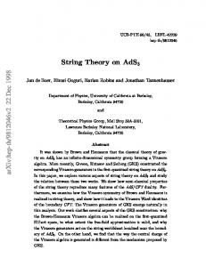
Figure 1: The string diagram of the spectral cover with interaction points Ii , i = 1..6. The interaction times τi and the angles θi define the location of the interaction points. The external states correspond to the marked points Pi , i = 1..4 at interaction points. For strings of length 2π the radii of the cylinders are identified with the momenta p+ in the light cone frame. A defining property of the Mandelstam diagram of a Riemann surface is the existence of a time axis τ and of periodic angular coordinates σ on each of the cylinders. The complex variable defined by w = τ + iσ parameterizes each of the cylinders. A Mandelstam diagram is uniquely specified by its interaction points where dw vanishes, gS internal momenta and gS internal shifts. On the whole this provides 3gs − 3 + p complex coordinates forming a cover of the moduli space of marked Riemann surfaces [16]. Finding these parameters will allow us to construct the Mandelstam diagram associated to the interaction of strings on the spectral cover. The construction of a Mandelstam diagram has to be adapted to the case of the spectral cover. Let us use the function w(λ) ˜ =

Z

λ

π ∗ Xd

(34)

defined up to the periods of π ∗ Xd . Consider now the real part τ˜ = Re(w) ˜ 12

(35)

up to the real parts of the periods. This real function has critical points at the zeros Ii with an index −14 . At the poles one sees that τ˜ → ±∞. The function τ˜ is a Morse function allowing to stratify the spectral cover according to its level sets. The image of the spectral cover under w˜ is interpreted as a string diagram with interaction points at the zeros Ii corresponding to the splitting or joining of two strings. Topologically this string diagram is defined by 2gS + p − 3 complex coordinates corresponding to the interaction points The position of the interaction points is specified by the interaction times and the twist angles along 2gs − 3 + p branches of the string diagram (fig. 1). The spectral cover can be given a metric using the string diagram. Let us define the flat metric dwd ˜ w˜ on the spectral cover. This is the induced metric from the flat metric on the string diagram. On the spectral cover we obtain gλλ¯ = |λ

dz 2 | dλ

(36)

Due to the holomorphy of the zweilbein wλ = λdz/dλ the metric is almost flat apart from the zeros and the poles creating a delta function singularity in the curvature R(Q) = 2π

2gSX −2+p i=1

δ(Q − Ii ) − 2π

p X i=1

δ(Q − Pi )

(37)

Of course the integral of the curvature gives the Euler characteristic. This is consistent with the string interpretation of the string diagram where the strings are flat cylinders joining at the interaction points. The string diagram defines the dynamics of the string interactions, i.e. a contact interaction at the interaction points. The kinematics of the strings is not yet specified as we have not explicitly described the momenta of the incoming and outgoing strings. This is provided by the addition of Wilson lines on the spectral cover. Up to now we have not taken into account the discrete ZN twists along homology cycles which can be turned on in the construction of flat bundles. This corresponds to adding different twisted sectors in the quotient U(1)/ZN . The flat vector bundle with the gauge connection A can be viewed as the quotient ˆ × su(N) × S1 )/ ∼ where Σ ˆ is the universal cover of Σ, su(N) the Lie al(Σ gebra of SU(N) and S1 the unit circle. The equivalence relation is (x, u, θ) ∼ ˆ as covering transformation (γ(x), adj(γ)u, θ) where γ is a loop on Σ acting on Σ and adj(γ) is the monodromy in the adjoint representation. Notice that the S1 factor is not involved in the quotient. One can define a twisted version of the R equivalence relation (x, u, θ) ∼ (γ(x), adj(γ)u, θ+ π−1 (γ) aS ) obtained by integrating a U(1)/ZN connection aS on S along the inverse image of γ. This twisting modifies the U(1) part of the gauge connection. It does not change the field X. 4

This gives a contribution 2 − 2gS − p to the Euler characteristic.

13

Let us consider a U(1) bundle over the spectral cover S that we endow with a flat connection aS . The building of such a flat vector bundle is characterized by maps in Hom(π1 (S), U(1)). This corresponds to having different winding numbers along the non-trivial loops of S. The flat vector bundle is modeled on the bundle (S˜ × U(1))/ ∼ where ∼ is the equivalence relation (x, θ) ∼ (γ(x), θ + 2πdγ ), S˜ is the universal cover of S and θ is an angle. The winding number dγ depends on the loop γ which acts on x as a covering transformation. We can now easily incorporate the ZN orbifold characterized by maps in Hom(π1 (S), ZN ). For a given loop γ in π1 (S) one can define a twisted action with twist 2πk/N by θ → θ + 2πk/N, k ∈ [0, N − 1]. The range of k is extended to the whole integers by taking into account the non-trivial winding numbers. As the fundamental group of the spectral cover is of dimension 2gS this gives N 2gS sectors. Physically these discrete transformations are discrete Wilson lines in the U(1) part of the gauge theory. One can always construct such a flat U(1) gauge field aS . Put aS = b + ¯b P S where b is a holomorphic one form b = gi=1 ui ωi and the one forms ωi form a basis of holomorphic Abelian differentials. Now we prescribe the Wilson lines Z

ai

aS =

2πki , N

Z

bi

aS =

2πki′ . N

(38)

The complex coefficients ui are always uniquely defined as the period matrix R Ωij = bj ωi has an invertible imaginary part. One obtains the push-down of aS ¯ i )dλ ¯ i where to Σ as π∗ aS = (ad ), i.e. a diagonal matrix of one forms b(λi )dλi + ¯b(λ ¯ λ. ¯ This matrix possesses monodromies around the branch aS = b(λ)dλ + ¯b(λ)d points corresponding to the exchange of the different sheets. The U(1) gauge field aΣ = tr(π∗ aS )IN ×N (39) defines a U(1) flat gauge connection on Σ. This connection is diagonally embedded in U(N). The total gauge connection is the sum of aΣ and the connection (16). As will be recalled in the next section the semi-classical evaluation of the matrix string path integral involves a residual U(1) gauge field a [6] living on the spectral cover. The other fields correspond to strings degrees of freedom in the Green-Schwarz formulation. Considering the Hamiltonian picture of this theory on the spectral cover the physical states are identified with light cone string states carrying some information coming from the quantization of the extra U(1) factor. The discrete Wilson lines modify the behaviour of the string states propagating along the string diagram of the spectral cover. Given a state |α > located at a non-trivial ai loop on the string diagram (fig. 1) and going along the cycle ai transforms the string state |α > into e2πiki /N |α >. Normalizing the string length to 2π we find that the state |α > acquires a momentum ki /N. Similarly the same 14

a1

b1 a2

b2

Figure 2: The equivalent Mandelstam diagram to the spectral cover where the momenta along the cycles ai , i = 1, 2 and the twist angles along the cycles bi , i = 1, 2 are quantized ′

state transported along the cycle bi picks up a phase e2πiki /N corresponding to a shift of the origin of the string by ki′ /N. The marked points correspond to the location of the external vertex operators. One can open up a small disc around each marked point to obtain a puncture. The punctures lead to (p−1) extra cycles. The (p−1) cycles around the punctures give quantized external momenta ki′′ . This is achieved by modifying the U(1) flat connection demanding that Z 2πki′′ (40) aS = N γi where γi are the p cycles around the punctures. One can always find the gauge P S P connection as aS = b + ¯b where b = gi=1 uiωi + pi=1 vi ωP0 Pi and ωP0 Pi is a meromorphic one form with poles at Pi and P0 with residues one and minus one respectively. The periods of these one forms ωP0 Pi are imaginary along the a and b cycles. Requiring that b is holomorphic at P0 implies the momentum P conservation pi=1 ki′′ = 0. The picture emerging from the description of the spectral cover fits with what is expected from light cone string theory[20]. First of all the continuous part of the construction leads to the spectral cover and its interpretation as a string diagram for closed strings. The parameterization of the spectral cover in terms of the coordinates of the interaction points specifies the interaction times and 2gs − 3 + p shifts. The discrete part of the construction, i.e. the assignment of ZN elements to the 2gS + p − 1 non-trivial cycles is equivalent to prescribing the internal and the external momenta in a quantized fashion. The strings are also twisted along the b cycles with discrete shifts sa , a = 1 . . . gS . 15

With this information we can construct the Mandelstam diagram of the spectral cover S. One can assign to all the p external cylinders and the (3gS − 3 + p) internal cylinders a radius equal to the quantized momentum α as determined by momentum conservation. This requires to define new coordinates on each of the cylinders by rescaling w˜ by α/L where L is the radius measured using the coordinates w. ˜ The radius of each of the cylinders is now α. Globally one patches up the new coordinates w on each of the cylinders by imposing that going around the b cycles the imaginary part of w is shifted by sa . The coordinates w = τ + iσ

(41)

built this way are defined globally and describe the Mandelstam diagram. The coordinates of the interaction points are now wi = τi + iσi , i = 1 . . . 2gS − 3 + p. The Mandelstam diagram of S has been built by joining the p external cylinders and the 3gS − 3 + p internal cylinders. The relative orientation of the flat cylinders is prescribed by the different shifts σi i = 1 . . . (2gS − 3 + p) and sa a = 1 . . . gS . The length of the cylinders is given by the interaction times τi . In another parameterization which will be useful when identifying the measure over the instanton moduli space one can utilize the twisting angles θi = 2π

sa σi , ηa = 2π αi αa

(42)

where the αi ’s and the αa ’s are the quantized momenta along the corresponding internal cylinders. We have thus constructed a Mandelstam diagram from the coordinates of the interactions points Ii and the quantized external and internal momenta. Deformations of the Mandelstam diagram by varying the positions of the interaction points, the shifts and the momenta correspond to changing the parameters of the instantons. On the whole we have identified the moduli space of instantons as a discretization of the moduli space of marked Riemann surfaces. This result had already be obtained in [11] using independent arguments. Here we have shown how this decomposition is intimately linked to the moduli space of matrix string instantons. In the next section we will study the dynamics of the string interactions more carefully and come back to the essential U(1) factor in the semi-classical approximation.

4

The Scattering Amplitudes

The path integrals of matrix models can be evaluated in a semi-classical fashion in the small string coupling limit[6]. The objects of interest are the scattering 16

amplitudes defined by the path integral A(1, ...., n) =

Z

DADXDΘφ(0)φ(∞)V1...Vv−2 e−S(X,A,Θ) .

(43)

The vertex operators are the analogue of the light cone string vertex operators. We also have inserted a wave function at both ends of the cylinder. These wave functions depend on the boundary values of the fields on the external circles. The link between the vertex operators and the wave functions is the usual one, i.e. obtained by integration over all the field configurations on a small disc with a vertex operator inserted at its centre. The vertex operators only involve the diagonal part of the fields in a suitable gauge. The string interpretation of the scattering amplitudes involves the semi-classical evaluation and the lifting of the action to the spectral cover. Let us first deal with the action in the semi-classical regime [6]. We expand the action around the instantons. The instantonic configuration (A, X) is taken in the gauge where the bosonic field Xd is diagonal. This amounts to applying a multivalued gauge transformation U −1 to all the fields. In particular the diagonal fluctuations xid are multivalued due to the non-trivial monodromies at the branch points. The path integral measure needs to be defined by fixing a gauge and introducing Faddeev-Popov ghosts. The gauge is fixed by ¯ w + ig 2 ([Xd , x¯] + [X ¯ d , x]). Gww¯ = ∂aw¯ + ∂a

(44)

Capital letters are only used for the background instantons. The Fadeev-Popov action is Z δG 1 tr( d2 w¯ c c) (45) SF P = − 2 2πg δǫ where ǫ is the gauge variation parameter. The gauge fixing is simply SGF =

1 tr( 4πg 2

Z

d2 wG2 ).

(46)

The fields are defined by an appropriate rescaling. The diagonal fields ad , cd are rescaled by a factor of g. Aw = gadw + and w , X = Xd + xd +

xI θnd xnd , X I = xId + nd , Θ = θd + √ g g g

(47)

where I = 3..8 are the directions transverse to the instanton. The ghosts are likewise √ (48) c = gcd + gcnd

17

and similarly for c¯. The Euclidean action becomes 1 S = Sd + Snd + O( √ ) g

(49)

The non-diagonal action Snd is quadratic and can be integrated out giving unity by supersymmetry. The higher order terms are all suppressed by the gauge coupling constant. In the small string coupling limit we are left with a purely diagonal path integral. The normalization of the diagonal fields has been chosen in such a way that the quadratic action is independent of the string coupling constant. The evaluation of the path integral is not trivial due to the multivalued nature of the diagonal fields. To obtain single-valued fields one needs to lift the fields to the spectral cover. The spectral cover is defined by considering the instanton on the Riemann sphere Σ and pulling it back to the cylinder C via the conformal mapping f : C → Σ. One gets XC = f ∗ XΣ . The spectral cover of the cylinder is then obtain from the eigenvalue equation det(λ −XC ) = 0. This allows use to use the previous results and lift the fields from the Riemann sphere to the spectral cover. The diagonal vectors xdj , j = 1 . . . N define a section x of a line bundle on the spectral cover S by the rule x(λi (z)) = xi (z) where λi (z) is the ith eigenvalue of Xd at z. Similarly the gauge field is lifted to the spectral cover leading to a one form ai (z) = a(λi )dλi /dω. This leaves us with an action defined on the spectral cover S for the bosonic fields 1 ( π

Z

¯

d2 λg λλ ∂λ aλ¯ ∂λ¯ aλ +

Z

d2 λ∂λ xId ∂λ¯ xId )

(50)

The integration is over S. Notice that the metric vanishes at the interaction points. At these points the inverse metric is ill defined and the semi-classical approximation breaks down. The action for the ghost fermions c, c¯ is easily derived Z 1 ¯ d2 λ∂¯ c∂c (51) π The ghost fields are anticommuting scalars on the spectral cover. We can now turn to the space time fermions. As defined in the path integral over the cylinder these fields are anticommuting scalars on the world sheet. They can be promoted to world sheet fermions on the spectral cover. This requires the use of the one form ωλ and its square root. The square root of the one form ωλ requires the choice of a spin structure on the spectral cover. This amounts to choosing the square root along non-trivial cycles. The spin structure is specified by 2gS signs corresponding to such a choice. Once a spin structure has been chosen it is called even if the product of the 2gS signs is even and odd in the opposite case. This endows the spectral cover with the structure of a super-Riemann 18

surface. To maintain the physical interpretation of the space-time fermions we impose that the square root of ωλ picks up a minus sign on all the possible cycles of the string diagram. The spin structure is then even. This allows to transform the space time fermions into world sheet fermions with values in the spin representations of SO(8) √ √ ¯ λ θα˙ . (52) ψ α = ωλ θα , ψ¯α˙ = ω The action for the fermions ψ, ψ¯ is lifted to the spectral cover to give the usual Dirac action i Z 2 ¯α˙ ¯ ¯ α ). d λ(ψ ∂ ψα˙ + ψ α ∂ψ (53) π Notice that the choice of the spin structure implies that there are cuts ending at the interaction points and the marked points. On the whole we find that the end-result of the semi-classical approximation is to produce a theory defined on the spectral cover of the matrix string instantons. Once the spectral cover is specified the theory is given by the light-cone GreenSchwarz action for space-time bosons and fermions. The space time fermions are also world sheet fermions on the spectral cover. This theory is coupled to a U(1) theory. Before completing the analysis of the path integral it is noteworthy to consider the Hamiltonian formulation of the theory. This is most conveniently achieved by considering the flat coordinates w˜ and the time axis τ˜ on the string diagrams. Using these coordinates the actions for the scalars, fermions and gauge fields reduce to free field theories defined on the flat cylinders forming the string diagrams. In the Hamiltonian picture there are Green-Schwarz string states |GS > propagating along each of these cylinders and interacting at the interaction points. Because of the presence of non-trivial U(1) backgrounds aS the intermediate states |α > are also characterized by fractional momenta α on all the internal and external cylinders. There are also fractional shifts sa for gS internal cylinders. The Hilbert space of the theory is H = HGS ⊗ R (54) where HGS is the Hilbert space of the GS states |GS > and R is the Hilbert space deduced from the quantization of the U(1) theory. Consider one of the cylinders on the spectral cover, we normalize its radius to L. The corresponding U(1) action is then 1 Z 2πL d˜ τ d˜ σ(∂0 a1 )2 2πg 2 0

(55)

in the gauge a0 = 0. In this gauge it is convenient to introduce the Wilson line g = e2πiLa1 19

(56)

at a given time τ˜ for σ ˜ independent gauge fields. In terms of this Wilson line the action reads Z 1 d˜ τ |g| ˙2 (57) 2 2 4π Lg and the Hamiltonian H = 4π 2 Lg 2 |p|2 . (58) This is the Hamiltonian of a free particle on a circle. The motion of this free particle depends on the different types of boundary conditions, i.e. on the discrete Wilson lines. In the untwisted sector the circle is identical to R/2πZ. In the twisted sectors with a Wilson line k/N the eigenvectors pick up a phase e2πik/N . In all cases denoting by θ the angular variable the momentum reads i∂/∂θ with eigenvectors e2πi(n+k/N )θ . The states |n, k > associated to these eigenvectors form a basis of the U(1) Hilbert space on the cylinder. There is one more subtlety due to the possible shifts si along the bi cycles bording the cylinder. The Hilbert space R is spanned by all the |n, k, si > which are eigenstates of H on the different cylinders and having a monodromy e2πisi along the bi cycles. Let us come back to the energy associated to these eigenstates. It simply reads H|n, k, si >= 4π 2 Lg 2 (n + k/N)2 |n, k, si > . (59) Combined with the eigenstates of the GS Hamiltonian H0 acting on light cone GS states we obtain eigenstates spanning the Hilbert space H. The total Hamiltonian reads HT = H + H0 . The propagation of the eigenstates from one end of the cylinder to the other end gives the evolution operator in Euclidean time e−τ (4π

2 Lg 2 (n+k/N )2 +(pI )2 +m2 )

(60)

where m is the mass of the GS state and pI its transverse momentum. Notice that the corrections to the GS eigenvalues are non-perturbative and of order 1/gs2 . In the limit gs → 0 the only non-vanishing terms satisfy n = 0, i.e. the contributions from the winding modes decouple. Moreover the non-perturbative corrections to the string scattering amplitude vanish altogether provided gs2N 2 /L → ∞. For the long strings where L ∝ N the most stringent condition is then gs2 N → ∞.

(61)

In the finite gs and N cases the string amplitude is corrected by non-perturbative contributions coming from the creation of D0 branes. To study the string scattering amplitude we change coordinates and use the w coordinates. In these coordinates the radius of each cylinder is equal to the momentum α = k/N. The light cone Hamiltonian whose bosonic part is 1 2π

Z

0

2πα

dσ((

∂xId 2 ∂xI ) + ( d )2 ) ∂τ ∂σ 20

(62)

has eigenvalues 2p− where p− =

(pI )2 + m2 . 2α

(63)

e−2ip− τ

(64)

The evolution operator is now where we have performed a Wick rotation on the world sheet. This evolution operator coincides with the light cone string field evolution operator. More precisely the evolution operator is associated to the Hamiltonian[16] K = iα

∂ − H0 . ∂τ

(65)

This Hamiltonian is easily identified with the light cone string field Hamiltonian with the canonical quantization rule [x± , p∓ ] = i yielding p− = −i∂/∂x− . We obtain the following x+ = 2τ. (66) Similarly with p+ ≡ α = −i∂/∂x− we find that the x− coordinate is periodic, the radius of the circle parameterized by x− is R− = N.

(67)

This completes the identification of the small string coupling regime of matrix string theory with light cone string theory where the radius R− goes to infinity with N. In conclusion we have seen that the large N limit is necessary in order to decouple non-perturbative effects and decompactify the x− direction. We can now make the above picture global. To do so we use the global coordinates w patched up to construct the Mandelstam diagram. By inserting a complete set of observables at the internal ends of the cylinders we build the scattering amplitude by propagating the states with the e−2iτi p− evolution operator on each internal cylinder. We still have to specify the interaction vertices. This necessitates to study the ghost action and its zero modes.

5

Picture Changing Operators and Supermoduli

The usual rules of string perturbation theory prescribe the inclusion of picture changing operators at the string interaction points[4]. In the RNS string context the picture changing operators appear after integrating over the supermoduli[13, 14]. To do so one deforms the super-Riemann surface structure by an anticom¯ to be equal to muting −1/2 tensor v and fix the two-dimensional gravitino field ∂v a linear combination of the super-moduli. The deformation of the super-Riemann 21

surface induces a supersymmetry transformation of the bosons and fermions. This leads to a direct coupling of the gravitino to the supersymmetric current. The integration over the components of the gravitino yields an insertion of the supersymmetric current at all the interaction points and hence the picture changing operators. In this section we will repeat parts of this construction. The deformation of the super-Riemann surface will lead to the inclusion of the picture changing operators at the interaction points as already discussed in the DVV paper. In the following we shall need to integrate functionally over various types of tensors on S. We define it by considering the Hilbert space of square integrable n tensors defined by the scalar product (φn , ψn ) =

Z

d2 λ(gλλ¯ )1−n φ¯n ψn .

(68)

Imposing that the integral is well-defined in the vicinity of the interaction points implies that for meromorphic tensors such that φn ∼ 1/λp one should verify that p < 2 − n. Functions can have at most a pole at the interaction points. The spinors n = 1/2 can also develop a pole. The one-forms have to be holomorphic while the quadratic differentials have to vanish. The same analysis in the vicinity of a marked point where the metric admits a pole implies that p < n. Thus functions have to vanish at the marked points while tensors of higher degrees can either be constant for n = 1 or have a pole n ≥ 2. Let us now study the normalizable ghost zero modes. The gauge fields (aλ , aλ¯ ) have been lifted to the spectral cover where they become single-valued. This entails that the only normalizable zero modes of the gauge fields are the gS holomorphic differentials. This is different for the ghosts. Indeed there are zero modes of the fermionic ghosts which are normalizable though not single-valued on the spectral cover. These zero modes are solutions of ¯ =0 ∂c

(69)

corresponding to meromorphic 1/2 tensors ψ1/2 on the spectral cover under the −1/2 world sheet boson-fermion correspondence sending ψ1/2 → ωλ ψ1/2 . These meromorphic zero modes ψ1/2 are well defined on the whole spectral cover apart from possible singularities at the interaction points where the metric vanishes. Their images under the boson-fermion correspondence yield (2gS − 2 + p) multivalued ghost zero modes5 . It is easy to construct the zero modes ψ1/2 in the case of an even spin structure. One can find for each of the 2gS − 2 + p interaction points a single zero mode 5

One can also find gS meromorphic zero modes obtained from the gS holomorphic differentials. The integration over the ghost fields is defined by discarding, in a similar way to the integration over the gauge fields, these gS meromorphic zero modes.

22

with a simple pole with residue one located at one of the interaction points Ii , the Szego kernel SIi (λ). This leads to a 2gS − 2 + p family of ghost zero modes. These zero modes ψ 1 are in one to one correspondence with the super-moduli of 2 the spectral cover, i.e. the holomorphic 3/2 differentials ψ 3 = ωλ ψ 1 . 2

(70)

2

The integration over the ghosts (c, c¯) is obtained by decomposing the zero modes P −1/2 c = a ma ωλ ψ a1 where the ψ a1 form a basis of the zero modes. The coordinates 2 2 ma are the anticommuting super-moduli coordinates. The measure of integration over the zero modes is (

Y

−1

dma dm ¯ a )| det(ψ a1 , ψ b1 )| 2

a

2

(71)

where the integration is over the anticommuting variables (ma , m ¯ a ). The light cone Green-Schwarz action possesses a supersymmetry ¯ I δξ xI = ξ α γαI α˙ ψ α˙ , δξ ψα˙ = ξ α γαI α˙ ∂x

(72)

where ξ α is a spinor. In particular the variation of the action under this supersymmetry reads Z 1 d2 λ∂ξ α Jα (73) δξ S = − π where we have defined ¯ I ψ α˙ . (74) Jα = γαI α˙ ∂x The derivative χα = ∂ξ α

(75)

plays the role of a gravitino. Similar expressions can be written with Jα˙ . The gravitino field is a classical field which encapsulates the super- Riemann surface status. In particular the light-cone Green-Schwarz action is written for χ = 0. The deformation of the super-Riemann structure induces a non-zero value for the gravitino field. Consider a (0, −1/2) anticommuting tensor v which parameterizes the deformation of the super-Riemann surface. Using a local basis 1/2 for the spinors uα , e.g. a local section of the bundle KS ⊗ S+ where S+ is the vector bundle modeled on the spin representation of SO(8) is of the form ψ α = ψ ⊗ uα , we can define the supersymmetry parameter ξ α = vuα

(76)

The action is not invariant under the supersymmetry transformations parameterized by ξ α . The scattering amplitude is only invariant if the expansion of the 23

gravitino field is chosen to involve the supermoduli which are explicitly integrated over 2gsX −2+p

α

χ =(

i=1

mi χi ) ⊗ uα

(77)

where the χi ’s define a slice of the supermoduli space. They form a basis of the (1, −1/2) tensors. The coupling of the gravitino field to the supercurrent leads to a sum of terms in correspondence with each of the interaction points mi Z 2 i α d λχ u Jα . − π

(78)

Integrating over the supermoduli is now easy, it amounts to expanding the exponential of the action and picking the linear terms in the supermoduli. This leads to the following insertion at each of the interaction points Z

¯ IΣ ¯I d2 λχi ∂x

(79)

where we have define the world-sheet fermion with values in the vector representation of SO(8) ¯ I = γ I uα ψ α˙ . Σ (80) αα˙ A convenient choice for the χi ’s is to be δ-function supported[14] leading to the insertion of ¯ IΣ ¯I ∂xI ΣI ⊗ ∂x (81) at the interaction point Ii . We have included the left and right sectors. This is the operator insertion introduced in DVV. Having identified the interaction generated by the integration over the supermoduli let us come back to the origin of the field ΣI . As defined it involves a local section of the SO(8) spin bundle uα . Introducing the twist field 1 σ=√ ωλ

(82)

and using the section uα one can define the world-sheet spinor Σα˙ = σuα˙

(83)

from which one can derive the operator product expansion γI ψ α (λ)ΣI (0) ∼ √αα˙ Σα˙ (0) λ

(84)

in the neighbourhood of one of the interaction points. Of course this identifies the pair (ΣI , Σα˙ ) with the spin fields associated to ψ α . 24

Finally let us comment on the ambiguities of the integration over the supermoduli. The insertion of the picture changing operator is intimately linked to the choice of the basis χi . Another choice for the χi ’s result in a different result after integration over the supermoduli. As in the case of superstring perturbation theory this ambiguity might only be resolved by a global definition of the integration over the supermoduli space.

6

The Large N Limit of the Scattering Amplitudes

We have now identified the scattering amplitudes in matrix string theory with a discrete version of the light cone string scattering amplitudes. The discretization appears in the x− sector of the theory. Moreover we have reproduced the DVV operator insertion at the string interaction points. In this section we consider the issue of the integration measure over the instanton moduli and the link with the Weil-Petersson measure. In the path integral we consider a background Abelian gauge field aS as defined in section 3 and expand around this background configuration. One has to sum over all the possible Wilson lines to take into account the different possible backgrounds. In the small coupling regime the contribution from the background gauge field decouples leaving a Gaussian integral defined by excluding from the path integration over the one-form aλ the zero modes due to the gS holomorphic Abelian differentials on the spectral cover. The result of the Gaussian integral is given by the determinant of ∆1 acting on one-forms. There is a correspondence φ1 → φ1 /ωλ between the normalizable eigenvectors φ1 of ∆1 and the normalizable eigenvectors φ0 of the Laplacian on scalars ∆0 for non-vanishing eigenvalues. This gives for the integral over aλ 1 det′ ∆0

(85)

The constant zero mode is not in the Hilbert space as it is not a normalizable mode. Similarly the integral over the eight scalar coordinates leads to a factor 1 ′4

det ∆0

(86)

Combining the two determinants we find a factor of 1 ′5

det ∆0

(87)

The quadratic action of the ghost field leads to a Gaussian integration over nonzero modes. The resulting integration yields the determinant of the Laplacian 25

operator acting on scalars det ′ (∆0 ).

(88)

Combined with the integration over the space time fermions we get a factor of ′5

det

(∆0 ).

(89)

cancelling the bosonic determinants. Let us now come to grips with the integration over the matter fields xd and ¯ Recall that the fermions (ψ, ψ) ¯ are world-sheet fermions on the spectral (ψ, ψ). cover with values in the spin representations of SO(8). We use the Mandelstam ¯ I , ψ α , ψ¯α˙ ) and the following coordinates w. Consider now a polynomial P (∂xId , ∂x d vertex operator ¯ I , ψ α , ψ¯α˙ )eipI xId V = P (∂xId , ∂x (90) d corresponding to the insertion of states |phys >= V |0 > with momentum pI at one of the marked points of the spectral cover. These vertex operators allow to define the string wave functions which are inserted at the end of the open cylinders of the Mandelstam diagram. The open cylinders are obtained using a cut-off limiting the length of the external cylinders. The ends of the open cylinders are located at times τa . Consider the wave function specified by the boundary string configuration (xId = x0 , ψ = ψ0 , ψ¯ = ψ¯0 ) at the end of an external cylinder φa (x0 , ψ0 , ψ¯0 , τa ) =

Z

x0 ,ψ0 ,ψ¯0

I ¯ DxId Dψα D ψ¯α˙ Va e−S(xd ,ψα ,ψα˙ )

(91)

obtained by integrating over the fields defined on the infinite cylinder τ ∈ [−∞, τa ] and the disc closing the cylinder at infinity where the vertex operator Va is inserted. The explicit dependence on the stopping times τa of the wave function φi (τa ) is removed by inserting the propagator[16] − φa (x0 , ψ0 , ψ¯0 ) = e−2ipa τa φa (x0 , ψ0 , ψ¯0 , τa )

(92)

− I where (p+ a , pa , pa ) is the momentum of the state inserted at the marked point Pa . The momentum p+ a appears explicitly in the construction of the Mandelstam I diagram, the momentum p− a is explicit in the wave function φa while pa completes the mass shell condition. The scattering amplitude is obtained by integrating the wave functions φa over the space-time fields (xId , ψα , ψ¯α˙ ) subject to the boundary conditions (x0 , ψ0 , ψ¯0 ) at the end of the external cylinders

Z

DxId Dψα D ψ¯α˙ (

2gSY −2+p i=1

Vi )(

p Y

I

¯

φa )e−S(xd ,ψα ,ψα˙ ) =


(93)

a=1

where the DVV operators Vi have been inserted at the interaction points 6 . 6

There is a vanishing factor coming from the Liouville Q to the non-chiral splitting Q action due of the Laplacian acting on fermions. It is given by (( i ρ(Pi ))/( i ρ(Ii )))−1/3 where ρ is the Weyl factor. This term has to be absorbed in the definition of the path integral

26

We still have to take into account the sum over the classical instantons. This amounts to summing over the moduli space of the instantons. Moreover we must divide by the number of twisted sectors due to the twisting by Wilson lines. On the whole this leads to A=

1 N 2gS

X

k1 ...k2gS

Z

MR

dµ| det(ψ a1 , ψ b1 )| 2

2

−1




(94)

a=1

where dµ is the measure of the instanton moduli space. This measure specifies that one has to integrate over the coordinates of the interaction points of the Mandelstam diagram. A change of the parameters of the instantons amounts to moving the coordinates of the interaction points. Let us describe the zero modes associated to the variation of the interaction points, i.e. the tangent space to the moduli space[22]. Locally around an interaction point the spectral cover S0 is defined by 1 w˜0 = λ20 2

(95)

corresponding to a one form π0∗ Xd = λ0 dλ0 . Let us perturb this spectral cover and move the interaction point. The equation of the perturbed Sǫ reads 1 w˜0 = λ(λ − 4ǫ). 2

(96)

The interaction point is at λ∗ = 2ǫ. The one form associated to Sǫ is πǫ∗ Xd = (λ − 2ǫ)dλ. It is easy to see that (λ − ǫ)dλ = λ0 dλ0 implying that πǫ∗ Xd = π0∗ Xd − ǫφ

(97)

where φ = dλ, i.e. the one form defining S0 has been perturbed by φ. Notice that the perturbation is holomorphic on Sǫ . This is not the case when pulled back to S0 where it reads in the vicinity of the two singularities φ ∼ ±(

±iǫ/2 ))1/2 dλ0 . λ0 − (±iǫ)

(98) 1/2

These infinitesimal perturbations of SO are determined by the one form dλ0 /λ0 shifted away from the interaction points by ±iǫ. So the zero modes characterizing the tangent space to the moduli space are spanned by the analytic one forms with a square root divergence at the interaction points of the spectral cover. Globally √ these one forms are found to be ωλ ψ1/2 where ψ1/2 is one of the 2gS −2+p spinors with a pole at the the interaction points. This identifies the tangent space to the moduli space and emphasizes the crucial role played by the interaction points. In particular we retrieve the dimension of the moduli space 2gS − 3 + p measuring the relative positions of the interaction points. 27

The measure in terms of the coordinates wi of the interaction points is now dµ = | det(ψ a1 , ψ b1 )|( 2

2

2gSY −3+p

dwi dw¯i )

(99)

i=1

This is the measure on the flat cylinders forming the Mandelstam diagram. Notice that the determinant arising from the tangent space to the moduli space cancels the determinant coming from the supermoduli measure. Inserting this measure in A we find that the scattering amplitude is obtained by integrating over all the possible topologies of the string diagram as specified by the coordinates of the interaction points. The scattering amplitude A on a spectral cover of genus gS carries a factor of (1/g)2gS −2+p coming from the 2gS − 2 + p fermionic zero modes. This springs from the rescaling c → gc used in the semi-classical expansion. Now as the string coupling is inversely proportional to g we find that the scattering amplitude is weighted with a factor gs−χ(S) as it should in the string scattering expansion7 . Notice that this amounts to adding a factor of gs to each of the interaction points. So the scattering amplitude carries the appropriate factor of gs to be identified with the string amplitude. Together with the Hamiltonian picture of GS states propagating on the Mandelstam diagram this shows that the scattering amplitude of matrix string theory is similar to a discrete version of the usual type IIA superstring amplitude in the light cone gauge. Let us now investigate the N dependence of the scattering amplitude A. First of all the geometry of the spectral cover is independent of N. Indeed we have seen that the number of moduli is uniquely specified by the genus gS and the number of marked points p. Fixing gS and p in the large N limit one can study the amplitude on a prescribed string diagram. Now the Mandelstam diagram depends on the momenta and shifts due to the Wilson lines. In the large N limit these momenta and shifts cover the entire real line, the discretization step 1/N goes to zero. So we retrieve the light cone Mandelstam diagrams of string theory. In particular all the external and internal momenta become continuous. It is then easy to see that in the large N limit the discrete sums in A converge to Q S the integral over the measure ga=1 αa dηa dαa . On the whole, combining with the measure dµ, we reconstruct the Weil-Petersson measure over the moduli space of marked Riemann surfaces d WP = (

2gSY −3+p

αi dθi dτi )(

gS Y

αa dηa dαa )

(100)

a=1

i=1

in terms of the twisting angles θi and ηa (42). The convergence towards the Weil-Petersson measure is only a weak convergence. 7

Here the Euler characteristic χ(S) is defined for the open Riemann surface with punctures obtained after removing a disc around the marked points.

28

Having obtained the measure of the moduli space of curves in the large N limit we find that the scattering amplitude A coincides with the scattering amplitude of superstring theory in the light cone gauge.

7

Conclusion

We have given an explicit description of the moduli space of matrix string instantons. They are defined in terms of (2gS − 3 + p) continuous parameters in correspondence with the deformations of the spectral cover. The scattering amplitudes in matrix string theory are equivalent to string scattering amplitudes on a Mandelstam diagram where the interaction points are free to move while the momenta of the interacting strings are quantized due to the presence of discrete Wilson lines in the description of flat bundles. The interaction points are associated to the supermoduli describing the structure of Super-Riemann surface on the spectral cover. We have explicitly integrated over the supermoduli and retrieved the DVV insertion of the picture changing operators at the interaction points. Finally we have studied the large N limit and shown that the measure on the matrix string instanton moduli space converges to the Weil-Petersson measure on the moduli space of marked Riemann surfaces.

Acknowledgements: I would like to thank D. Bernard for useful comments on vector bundles and F. Nesti, P. Vanhove and T. Wynter for numerous discussions on matrix theory. This work was partially supported by the EU Training and Mobility of Researchers Program (Contract FMRX-CT96-0012).

29

References [1] R. Dijkgraff, E. Verlinde and H. Verlinde Nucl. Phys. B 500 (1997) 43. [2] E. D’Hoker and D. H. Phong Rev. Mod. Phys. Vol 60 (1988) 917. [3] T. Wynter Phys. Lett. B 415 (1997) 349 [4] S. Mandelstam Nucl. Phys. B 64 (1973) 205. [5] G. Bonelli, L. Bonora and F. Nesti Phys. Lett. B435 (1998) 303. [6] G. Bonelli, L. Bonora and F. Nesti Nucl. Phys. B 538 (1999) 100. [7] S. B. Giddings, F. Haquebord and E. Verlinde Nucl. Phys B 537 (1999) 260. [8] N. J. Hitchin Proc. Lond. Math. Soc. 55 (1987) 59. [9] N. J. Hitchin Topology 31 (1992) 449. [10] N. J. Hitchin Duke Math. J. 54 (1987) 255. [11] G. Bonelli, L. Bonora, F. Nesti and A. Tomasiello Matrix String Theory and its Moduli Space hep-th/9901093. [12] I. K. Kostov and P. Vanhove Phys. Lett B 444 (1998) 196. [13] E. Verlinde and H. Verlinde Phys. Lett B 192 (1987) 95. [14] E. Verlinde and H. Verlinde Lectures on String Perturbation Theory Trieste Spring Summer School on Superstrings, April 1988. [15] E. D’Hoker and S. B. Giddings Nucl. Phys. B 291 (1987) 90. [16] S. B. Giddings Fundamental Strings in Particles, Strings and Supernovae, proceedings of the 1988 Theoretical Advanced Study Institute, Brown University, eds. A. Jevicki and C. I. Tan (World Scientific, Singapore, 1989). [17] S. Kobayashi Differential Geometry of Complex Vector Bundles Princeton University press. [18] D. Bernard Nucl. Phys. B 309 (1988) 145. [19] R. Donagi Spectral Covers in current topics in complex algebraic geometry, Math. Scien. Res. Inst. Publ. 28 (Berkeley, CA1992/92) 65-86. [20] S. B. Giddings and S. A. Wolpert Comm. Math. Phys 109 (1987) 177. [21] N. Nekrasov Comm. Math. Phys. 180 (1996) 587. [22] T. Wynter High Energy Scattering Amplitudes in Matrix String Theory hep/th 9905087

30