May 21, 2013 - Neil Shenvi1, Helen Van Aggelen1,2, Yang Yang1, Weitao Yang1, ...... [21] E. G. Hohenstein, R. M. Parrish, and T. J. Martinez, J. Chem. Phys.
The tensor hypercontracted parametric reduced density matrix algorithm: coupled-cluster accuracy with O(r4 ) scaling Neil Shenvi1 , Helen Van Aggelen1,2 , Yang Yang1 , Weitao Yang1 , Christine Schwerdtfeger3 , and David Mazziotti4 1
Dept. of Chemistry, Duke University, Durham, NC 27708 Dept. of Inorganic and Physical Chemistry, Ghent University, 9000 Ghent, Belgium Dept. of Chemistry, The University of Illinois at Urbana-Champaign, Urbana, IL 61801 and 4 Dept. of Chemistry, The University of Chicago, Chicago, IL 60637 (Dated: May 22, 2013) 2
arXiv:1305.4802v1 [physics.chem-ph] 21 May 2013
3
Tensor hypercontraction is a method that allows the representation of a high-rank tensor as a product of lower-rank tensors. In this paper, we show how tensor hypercontraction can be applied to both the electron repulsion integral (ERI) tensor and the two-particle excitation amplitudes used in the parametric reduced density matrix (pRDM) algorithm. Because only O(r) auxiliary functions are needed in both of these approximations, our overall algorithm can be shown to scale as O(r4 ), where r is the number of single-particle basis functions. We apply our algorithm to several small molecules, hydrogen chains, and alkanes to demonstrate its low formal scaling and practical utility. Provided we use enough auxiliary functions, we obtain accuracy similar to that of the traditional pRDM algorithm, somewhere between that of CCSD and CCSD(T).
I.
INTRODUCTION
The problem of the rapid growth of the electronic wavefunction with system size has plagued quantum chemistry for decades[1, 2]. There have been many attempts to conquer the ‘curse of dimensionality’ and a large number of highly successful approximations have been developed. The simplest approach is the one taken by Hartree-Fock theory, which approximates the exact wavefunction as a single Slater determinant. Missing from the Hartree-Fock result is the effect of electronic correlation, which determines many of the atomic and molecular properties in which chemists are most interested. The difficulty inherent in electronic structure calculations is that correlated methods usually scale as higher orders of the number of basis functions involved in the calculation. A straightforward implementation of Hartree-Fock scales as O(r4 ) where r is the number of basis functions. Approximate methods employed to capture correlation face a trade-off between accuracy and efficiency[3, 4]. Perturbative treatments such as MP2 and MP4 scale as O(r5 ) and O(r6 ), respectively[3]. Configuration interaction methods, which add in double-, triple- and quadruple-order excitations, form a hierarchy of methods which scale as O(r6 ) and higher[5]. A plethora of other, highly accurate methods based on coupled-cluster theory[5, 6], 2-particle reduced density matrices[7–10], and reduced active space diagonalization[11] also scale as at least O(r6 ). Due to this high O(r6 ) scaling, these methods are generally not applicable beyond small molecules. Instead, quantum chemists have increasingly turned to density functional theory (DFT), which offers low O(r4 ) or even O(r3 ) formal scaling while managing to capture varying amounts of the electronic correlation[12, 13]. Nonetheless, the search for efficient wavefunction-based methods that are competitive with DFT has continued, motivated by the importance of strong correlation in many systems such as transition metal clusters, solid state devices, and molecules far from their equilibrium geometries. One approach which attempts to reduce both the cost and scaling of correlated electronic structure methods is the decomposition of the electronic repulsion integral (ERI) tensor, which is naturally a rank-4 object, into products of lower-rank objects. Resolution-of-the-identity techniques[14–17] are one subset of this approach, as are pseudospectral methods[18–20]. Recently, Hohenstein et al[21] introduced tensor hypercontraction density fitting (THC-DF) to decompose the electron repulsion integral tensor, an object which is central to ab initio electronic structure calculations. The authors showed that an auxiliary basis could be used to express the rank-4 ERI tensor as the product of five rank-2 tensors. This approach led to O(r4 ) algorithms for MP2, MP3[21], CC2[22], and -tentatively- for CISD and CCSD[23], where r is the number of one-particle basis functions. In the last case of the CISD and CCSD algorithms, the THC methodology has not yet been implemented in a fully O(r4 ) manner, but initial results were encouraging. In all of these cases, the application of tensor hypercontraction adds a non-negligible overhead and prefactor to the algorithm. However, the reduced asymptotic scaling will lead to a cross-over that renders the THC versions more efficient for sufficiently large systems. Concurrently, Mazziotti et al. have been developing a parametric reduced density matrix (pRDM) algorithm that can be used to obtain ground state electronic energies with an accuracy somewhere between CCSD and CCSD(T)[24– 26]. Applications have been made to studying the energy barrier of between oxywater and hydrogen peroxide[27], the relative populations of cis and trans carbonic acid at 210 K[28], the diradical barrier to rotation of cis and trans diazene[29], and the relative populations of olympicene and its isomers[30]. The algorithm was also explicitly
2 constructed to preserve size extensivity, an important feature of any method intended for application to large systems. However, the asymptotic scaling of the algorithm is O(r6 ), even when the excitation tensor is spectrally composed, due to the need for a linear number of terms in the spectral composition. In this paper, we show that the pRDM algorithm and the THC methodology can be combined to produce a tensor hypercontracted parametric reduced density matrix (THC-pRDM) algorithm that scales as O(r4 ). As in the work of Martinez et al., we will decompose both the ERI and the excitation tensors using THC. But we will apply these decompositions to the pRDM algorithm of Mazziotti et al., rather than to more traditional electronic structure methods like CISD or CCSD. We believe that our algorithm is the first example of a fully-implemented O(r4 ) methodology with CCSD-like accuracy. Our approach also has several intrinsic advantages. First, because it produces the ground state 2-RDM, calculations of one- and two-particle properties of the ground state are straightforward, in contrast to the complexity of such calculations in coupled-cluster algorithms[31]. Second, because RDM methods approach the problem of electronic structure differently than wavefunction-based methods, they provide a complementary perspective that can be valid when wavefunction-based methods are not. Finally, the RDM approach suggests several approximations which are not available or at least are not obvious in wavefunction-based methods. We discuss a few of these in Sec. IV. Our paper is organized as follows: in Sec. II, we outline the theoretical underpinnings of our algorithm. We review tensor hypercontraction and the pRDM algorithm and discuss several approximations that we make in the derivation of the THC-pRDM algorithm. In Sec. III, we show the results of applying our algorithm to several systems such as small molecules, hydrogen chains, and alkanes. We find that our algorithm shows the expected behavior, approaching the standard pRDM result as the number of auxiliary functions is increased. We also show that we do indeed obtain O(r4 ) scaling for large systems, albeit with a large prefactor. In Sec. IV, we present some conclusions and discuss future directions for increasing the efficiency and accuracy of our method. II. A.
THEORY
THC decomposition of the Hamiltonian
The electronic Hamiltonian of an atom or molecule can be written in 2nd-quantized notation as ˆ = H ˆ1 + H ˆ2 H X X ij † † 1 i † 2 = ǫk cˆi cˆk + ǫkl cˆi cˆj cˆl cˆk ik
(1) (2)
ijkl
where hik is the rank-2 matrix of 1-electron integrals and 2ǫij kl is the rank-4 electronic repulsion integral tensor defined by Z Z 1 2 ij ǫkl = φj (r2 )φl (r2 ) (3) dr1 dr2 φi (r1 )φk (r1 ) |r1 − r2 | The ERI tensor can be decomposed using a set of PH auxiliary functions as 2 ij ǫkl
= (ik|jl) =
PH X
(4)
hiP hkP JP Q hjQ hlQ .
(5)
P,Q=1
Martinez and coworkers have developed a number of approaches to find an efficient THC decomposition of the ERI tensor[21, 32, 33]. We chose to implement this decomposition in terms of a simple non-linear least-squares fitting procedure. First, we used the standard RI-V method to express the ERI tensor in terms of two rank-3 tensors, 2 ij ǫkl
=
P RI X
vµik wµν vνjl ,
(6)
µ,ν=1
where µ and ν label the PRI auxiliary density functions using the RI auxiliary basis found in the EMSL basis set exchange[34]. In the second step, we find some optimal set of auxiliary functions to decompose the rank-three tensor vµik , vµik =
PH X
P =1
hiP hkP uµP .
(7)
3 Molecule PH (THC) PH (exact) Ec (THC) Ec (exact) CO(cc-pVDZ,PA = 50) 194 465 308.17 307.81 H2O(cc-pVTZ, PA = 100) 292 2192 286.44 285.19 CH4(cc-pVDZ, PA = 50) 210 630 190.67 190.62 H8(cc-pVDZ, PA = 48) 178 820 171.34 171.18 TABLE I: Number of auxiliary functions PH and correlation energies Ec (in mH) using the THC compressed ERI tensor versus the exact ERI tensor. In all four cases, the error of the THC approximation was less than 2 mH.
This decomposition can be accomplished through optimization of the cost-function J=
X
vµik
ikµ
−
PH X
hiP hkP uµP
P =1
!2
(8)
with respect to the variables hiP and uµP . The evaluation of the cost function and its gradients requires O(r2 PRI PH ) operations, although optimization can require several thousand iterations. Having found an optimal hiP and uµP using a non-linear optimization scheme, the final THC decomposition is given by Eq. (5) where JP Q =
P RI X
uµP uνQ wµν
(9)
µ,ν=1
Provided that PRI and PH both scale as O(r), this entire process requires O(r4 ) operations, which has the same complexity as our THC-pRDM algorithm. In practice, we find that if PRI is between 2r and 4r and PH is between 4r and 6r, the THC decomposition leads to errors less than 2 mH in the ground state energies obtained, which is suffucient for our purposes. Table I shows a few representative molecules from our example and the ground state correlation energies obtained using the THC-compressed ERIs versus the exact ERIs. B.
THC decomposition of the excitation tensor
Configuration interaction and coupled cluster methods both rely on the use of an excitation operator which acts on some single-configuration Hartree-Fock reference wavefunction. If we let i, j, k, l label occupied orbitals and a, b, c, d label unoccupied orbitals in the reference state, then the excitation operator can be written as Tˆ = Tˆ1 + Tˆ2 X X 1 a † 2 ab † † Ti cˆa cˆi + Tij cˆa cˆb cˆj cˆi . = ia
(10) (11)
ijab
Spin symmetry can be taken into account explicitly; however, in this equation and what follows, we will ignore spin in order to simplify notation. For the THC-pRDM method, we will apply THC decomposition to the two-particle excitation operator Tˆ2 , modifying it slightly to take into account the differences between occupied and virtual orbitals. We then obtain 2 ab Tij
=
PA X
(yaR xiR zRS ybS xjS − yaR xjR zRS ybS xiS ).
(12)
R,S=1
Note that the second term in Eq. (12) is included to ensure the antisymmetry of the tensor Tˆ2 . The symmetry requirements of Tˆ2 also imply that zRS should be a symmetric matrix. By writing the excitation tensor in terms of a THC decomposition, we have been able to compress a rank-4 object 2Tijab into the product of three rank-2 objects, xiR , yaR , and zRS . A key to reducing the overall scaling of the electronic structure algorithm will be to determine how many auxiliary functions PA are needed to approximate the 2T tensor with sufficient accuracy. In Sec. III, we will show that we need only a linear number of auxiliary functions PA = O(r) to capture essentially all of the electronic correlation recovered by the standard pRDM algorithm, even though an exact representation of 2T would require PA = P (r2 ) auxiliary functions.
4 C.
The pRDM algorithm
The version of the pRDM algorithm that we will employ here was first introduced in [24] and subsequently refined in [25]. The algorithm is based on the construction of an optimal ground state 2-particle reduced density matrix (2-RDM), constrained to have a particular form parametrized by tensors 1T and 2T . The easiest way to understand the pRDM algorithm is to recognize that the 1- and 2-RDMs corresponding to a CISD wavefunction can be written exactly in terms of the excitation tensors 1T and 2T . Again using the notation that indices i, j, k, l represent occupied orbitals and a, b, c, d represent unoccupied orbitals, the RDMs for the Hartree-Fock reference state are Dki = δki
1
ij Dkl
2
=
δki δlj
(13) −
δli δkj
(14)
with all other elements equal to 0. Excitation out of this reference state adds cumulant components to the RDMs, which can be expressed in terms of 1T and 2T . Straightforward evaluation from the CISD wavefunction yields Dji = δji + 1∆ij
1
Dia 1 a Db 2 ij Dkl 2 ia Djk 2 ia Djb 2 ab Dkl 2 ia Dbc 2 ab Dcd 1
= = = = = = = =
(15)
∆ai 1 a ∆b δki δlj − δli δkj + 1∆ik δlj − 1∆il δkj δji 1∆ak − δki 1∆aj + 2∆ia jk δji 1∆ab − 1Tbi 1Taj + 2∆ia jb 2 ab ∆kl 2 ia ∆bc 2 ab ∆cd 1
(16) (17) − 1∆jk δli + 1∆jl δki + 2∆ij kl
(18) (19) (20) (21) (22) (23)
where the cumulants are given by 1 X 2 ab 2 ab X 1 a 1 a Tjk Tik − Ti Tj 2 a kab X 2 ab 1 b Tij Tj + 1Tia =
∆ij = −
(24)
∆ai
(25)
1
1
bj
∆ab =
1
1 X 2 ac 2 bc X 1 a 1 b Ti Ti T T + 2 cij ij ij i
1 X 2 ab 2 ab Tij Tkl 2 ab X 2 ab 1 b = Tjk Ti
∆ij kl =
2
∆ia jk
2
(26) (27) (28)
b
∆ia jb = −
2
∆ab ij =
2
∆ia bc =
2
X
2 ac 2 bc Tjk Tik
kc 2 ab Tij
X
2 bc 1 a Tij Tj
(29) (30) (31)
j
∆ab cd =
2
1 X 2 ab 2 cd T T 2 ij ij ij
(32)
The total energy of the system can then be calculated by tracing the 1- and 2-RDMs of the system over the 1- and 2-particle components of the Hamiltonian in Eq. (2), � � � � E = Tr 1D · 1ǫ + Tr 2D · 2ǫ (33)
5 Although Eqs. (15–23) are exact for CISD wavefunctions, modifying the cumulants in Eq. (25) and Eq. (30) while leaving the other cumulant unchanged can produce approximations to the ground state energy that are far more accurate than CISD[24, 25]. Using Cauchy-Schartz inequalities based on N -representability conditions[24, 35], we can generalize these two equations to include a functional of 1T and 2T , v u 1 1 X X X u 1 a 2 ab 1 b 1 at 2cp {p,q}Σa 3cp {p,q}Σa − (34) ∆i = Tij Tj + Ti 1 − q q i i ∆ab ij
2
p,q=0
p,q=0
bj
v u 1 2 X X u 2 ab t 3cp {p,q}Σab , 4cp {p,q}Σab − = Tij 1 − q q ij ij
(35)
p,q=0
p,q=0
where the Σ tensors can be written in terms of 1T and 2T,[25] X {0,0} a Σi = (1Tkc )2
(36)
kc
{1,0} a Σi
=
X
(1Tic )2
(37)
(1Tka )2
(38)
c
{0,1} a Σi {1,1} a Σi {0,0} ab Σij
= =
X
k 1 a 2 ( Ti )
(39)
1 X 2 cd 2 = ( Tkl ) 4
{1,0} ab Σij
=
{0,1} ab Σij
= 1∆aa + 1∆bb
{2,0} ab Σij
(42) (43)
∆ab ab 2 jb − ∆jb
(44)
=
{0,2} ab Σij
=
2
{1,1} ab Σij
= =
(41)
∆ij ij
2
{2,1} ab Σij
(40)
klcd −1∆ii − 1∆jj
X
2 ib 2 ia − 2∆ja ja − ∆ib − ∆ia
(45)
ij 2 (2Tbc )
(46)
ij 2 (2Tac )
+
c
{1,2} ab Σij {2,2} ab Σij
= =
X
jk 2 ik 2 (2Tab ) + (2Tab )
k 2 ab 2 ( Tij )
(47) (48)
The square-root factor in Eqs. (34) and (35) acts like a normalization constant for the elements of the 1- and 2-RDMs. Physical explanations of these quantities can be found in [25]. What is important to note is that the constants c{p,q} can be chosen arbitrarily to define different functionals that relate the excitation tensors 1T and 2T to the components of the 1- and 2-RDM. For instance, the choice 4c{0,0} = 3c{0,0} = 2c{0,0} = 1 with all other coefficients equal to zero yields precisely the CISD wavefunction[25]. Mazziotti and coworkers devised several other functionals, all of which are obtained by choosing different coefficients for 4c, 3c, and 2c (see Table II). To perform an energy calculation, we select a functional and then minimize the energy in Eq. (33) with respect to the tensors 1T and 2T . In this paper, we will focus on the M2 functional introduced by Mazziotti in [25], which was able to provide ground state energies with an accuracy somewhere between CCSD and CCSD(T) for a wide variety of molecular systems. One other distinction that will be important for the THC-pRDM algorithm is that the zeroth order and cumulant contributions to the total energy in Eq. (33) can be evaluated separately. For this reason, we choose to evaluate the Hartree-Fock energy and density matrix using the exact 2-electron ERIs rather than the RI-V or THC approximations. We invoke the THC approximation to the ERIs only when evaluating the energetic contribution of the cumulants. This choice is important since the absolute Hartree-Fock electronic energy is much larger than the correlation energy. Because we restrict our use of the THC approximation to the calculation of the correlation energy, we need a far less precise approximation of the ERIs to obtain an approximation of the total energy with sub-miliHartree accuracy.
6 Functional 4c00 4c10 4c20 4c11 4c21 4c22 3c00 CISD 1 0 0 0 0 0 1 CEPA 0 0 0 0 0 0 0 M2 0 1/5 3/5 -1/10 0 -3/5 0 M2′ 0 1/5 3/5 -1/10 0 0 0
3 1 3 1 2 0 2 1 2 1 c0 c1 c0 c0 c1
0 0 1 0 0 0 1 -1 0 1 -1 0
0 0 0 0 1 -1 1 -1
TABLE II: Selected 2-RDM functionals defined in [25] and in the current work. Coefficients not shown are specified by particle/hole duality (cpq = cqp ). To preserve O(r 4 ) computational scaling, a single term from the M2 functional must be truncated, yielding the M2′ functional. Table III shows that this change produces negligible differences in energy.
D.
Applying THC to the pRDM algorithm
The application of tensor hypercontraction to the pRDM algorithm is relatively straightforward. We first write the rank-4 ERI tensor as a THC decomposition, according to the methodology discussed in Sec. II A. If we also express the rank-4 excitation tensor 2T as a THC decomposition (see Eq. (12)), then we can calculate the energy contributions of most of the cumulants in Eqs. (24–32) in O(r4 ) operations. For instance, the energy contribution from the cumulant in Eq. (31) is X 2 ia 2 ia E = ǫbc ∆bc (49) iabc
=
X
′ ′ ′ ′ ′ ′ JP Q zRS ySQ JP Q zRS − x′SP TRQ yRP ySQ x′RP TSQ yRP
P QRS
�
(50)
where x′RP =
X
xiR hiP
(51)
yaR haP
(52)
xiR 1Tia haP .
(53)
i
′ yRP =
X a
′ TRP =
X ia
The derivative of the energy expression with respect to the elements xiR , yaR and zRS of the excitation operator can likewise be calculated in O(r4 ) operations. Only the cumulant contribution in Eq. (35) is potentially problematic and necessitates two simple approximations to preserve O(r4 ) scaling. First, we observe that the square-root operation in Eq. (35) is problematic because it inextricably entangles all four indices a, b, i, j in the tensor 2Tijab with the tensors {p,q}Σab ij . Unfortunately, the speed-up produced by the THC decomposition necessitates that these indices be disentangled into pairs of at most two indices. To solve this problem, we first approximate the square-root operation via Taylor expansion[25]. Provided that the excitation tensor 2T is relatively small in magnitude, which is the case for all systems close to their mean-field reference, this approximation should be negligible. Next, we observe that the {2, 1}, {1, 2} and {2, 2} terms in Eq. (35) entangle 3, 3, and 4 indices, again eliminating the possibility of an O(r4 ) evaluation. However, the M2 functional fortuitously sets the coefficients 4 {2,1} c and 4c{1,2} to zero. The only approximation we need to make is to additionally set 4c{2,2} = 0 (see Table II). This is not a significant approximation either, since all the elements of {2,2}Σab kl should be small if the system is close to its mean-field reference because each element in the class contains only one positive term. Table III shows that the effect of both of these approximations on the ground state energies for several representative systems is negligible, amounting to less than 0.2 mH. E.
The initial guess for the excitation tensor
One factor that can greatly improve algorithmic convergence is a choice of a good initial guess for the parameters xiR , yaR and zRS that compose the THC-pRDM excitation operator. The MP2 amplitudes for a given Hamiltonian
7 standard HCN(cc-pVDZ) 313.05 H2O(cc-pVTZ) 288.43 CH4(cc-pVDZ) 192.39 H8(cc-pVDZ) 172.32
Taylor 313.08 288.44 192.40 172.34
M2′ Taylor + M2′ 312.91 312.95 288.41 288.42 192.38 192.39 172.27 172.28
TABLE III: Comparison of the pRDM ground state energy under various approximations. The first column shows the result using the standard pRDM algorithm with the M2 functional. The second column uses a Taylor expansion of the functional M2 . The third column uses the M2′ functional with no Taylor expansion. The last column employs both approximations, corresponding to the approach taken by the THC-pRDM algorithm. The approximations produce negigible differences in the final energy for the systems studied.
are known analytically to be 2 ab Tij
= =
1 2 ab ǫ Fii + Fjj − Faa − Fbb ij Fii + Fjj
(54)
PH X 1 haP hiP JP Q hbQ hjQ − Faa − Fbb
(55)
P,Q=1
where F is the Fock matrix. However, we need to express these amplitudes in THC form. Here we follow [21] in writing the MP2 amplitudes as an integral and then applying Gauss-Laguerre quadrature to express them as a weighted sum over knot points. This procedure yields 2 ab Tij
=
=
Fii + Fjj Z
∞
dx
0
(56)
P,Q=1
PH X
haP hiP JP Q hbQ hjQ exp (−(Fii + Fjj − Faa − Fbb )x)
(57)
P,Q=1
1 = 2∆E ≈
PH X 1 haP hiP JP Q hbQ hjQ − Faa − Fbb
Z
∞
′
dx
0
PH X
haP hiP JP Q hbQ hjQ exp (−(Fii + Fjj − Faa − Fbb − 2∆E)x′ /2∆E) exp (−x′ )
(58)
P,Q=1
nk PH X 1 X wn h′aP,n h′iP,n JP Q h′bQ,n h′jQ,n 2∆E n=1
(59)
P,Q=1
where h′aP,n = exp ((Faa − ELUMO )x′n /2∆E) haP
(60)
h′iP,n
(61) (62)
EHOMO )x′n /2∆E) hiP
= exp (−(Fii − ∆E = EHOMO − ELUMO
and where (x′n , wn ) are a set of nk Gauss-Laguerre knot points and weights. From this expression, we can then define a cost function 2 PA X X 2Tijab − J = yaR xiR zRS ybS xjS (63) R,S=1
abij
≈
X abij
1 2∆E
nk X
n=1
wn
PH X
P,Q=1
h′aP,n h′iP,n JP Q h′bQ,n h′jQ,n −
PA X
R,S=1
2
yaR xiR zRS ybS xjS .
(64)
2 Eq. (64) and the derivatives of J with respect to xiR , yaR , and zRS can be evaluated in O(n2k PA PH ) operations. We find that nk = 8 provides sufficient accuracy for our purposes. And since PA and PH both scale as r, the entire optimization procedure will scale as O(r3 ). Because the MP2 amplitudes are not normalized, our initial condition must include a normalization factor zRS → αzRS that prevents the excitation amplitudes from growing increasingly large as the system size increases. We find that by using this guess, the initial MP2 guess will already recover a large fraction of the correlation energy and can dramatically reduce the convergence time of our algorithm.
8 Molecule PA = 20 CH2 139.91 CO 277.91 H2 O 207.42 HCN 274.69 N2 295.98 NH3 191.59
PA = 30 143.31 294.84 215.28 293.30 312.79 203.65
PA = 40 144.19 303.52 216.94 300.39 323.08 207.71
PA = 50 144.62 308.17 217.87 307.08 326.07 209.04
PA = ∞ 145.09 312.38 218.65 313.05 331.78 210.34
CCSD CCSD(T) 142.38 145.45 306.88 318.50 217.33 220.62 307.18 320.20 326.32 339.71 208.23 212.28
TABLE IV: Ground state correlation energies in mH for small molecules in the cc-pVDZ basis. As the number of auxiliary functions is increased, the THC-pRDM energy approaches the standard pRDM energy, which lies between the CCSD and CCSD(T) energies.
F.
The final THC-pRDM algorithm
Having discussed the various constituents of the THC-pRDM algorithm, we can now provide a complete outline: 1. Calculate the 1- and 2-electron integrals using a standard electronic structure package, such as QM4D, the package we used[36]. Use RI-V to also approximately express the ERIs in terms of auxiliary density functions (see Eq. (6)) 2. Minimize the cost function in Eq. (8) to obtain a good THC decomposition of the ERIs from the RI-V calculation 3. Perform standard Hartree-Fock using the exact ERIs to obtain the ground state energy and density matrix 4. Obtain the initial starting values for the matrices xiR , yaR , and zRS from the approximate MP2 amplitudes (see Sec. II E) 5. Select a normalization factor α which minimizes the energy of the initial MP2 guess 6. Minimize the energy with respect to xiR , yaR , zRS , and 1Tia using a non-linear optimization algorithm. Convergence can be improved by optimizing the variables in three steps: (xiR , yaR ), zRS , and 1Tia . The optimization process is repeated until a sufficient level of convergence is achieved. III.
RESULTS
We applied the THC-pRDM algorithm to a variety of molecular systems to test its accuracy. Our first concern was how quickly the THC-pRDM algorithm would approach the standard pRDM limit as we increased the number of auxiliary functions PA . Table IV shows the results of our calculations for a set of six small molecules in the cc-pVDZ basis. As the number PA of auxiliary functions is increased, the correlation energy does rapidly approach that of the standard pRDM algorithm. Table V shows the same six molecules in the cc-vPTZ basis and the same behavior is observed. In this case, the largest number of auxiliary functions yields an answer with greater accuracy than CCSD, except for the HCN molecule. It is encouraging to see that only about PA = 1.5r auxiliary functions are needed to obtain accuracy similar to that of CCSD in both basis sets. Still, the high symmetry of these small molecules and the fact that the number of electrons remains constant as the basis size is increased makes it difficult to extract any scaling information from these test cases. A more important test of scaling comes from the alkane series shown in Table VI. In this table, we report the percentage of the CCSD(T) correlation energy that can be obtained from THC-pRDM, standard pRDM and CCSD. In this table, we can clearly see that the number of auxiliary functions needed to obtain any particular level of accuracy scales linearly with N , the length of the carbon chain. The number of auxiliary functions needed to obtain CCSD-level accuracy also represents a huge compression of the excitation tensor. For instance, the excitation tensor for C4 H10 contains approximately 3 million independent parameters. In contrast, the THC compressed excitation operator with PA = 200 auxiliary functions contains approximately sixty thousand independent elements, yielding a compression factor of 50. Yet despite this compression, the THC-pRDM algorithm easily attains accuracy greater than the CCSD result. Similar behavior is shown in Table VII, where the algorithm was applied to linear hydrogen chains where the internuclear separation of each hydrogen was R = 0.74 ˚ A. Once again, the THC-pRDM algorithm required a number of auxiliary functions that scaled linearly with the number of atoms in the chain. Both of these results indicate that
9 Molecule PA = 40 CH2 173.31 CO 355.35 H2 O 272.69 HCN 349.78 N2 378.67 NH3 251.65
PA = 60 180.13 381.59 281.02 370.50 401.71 263.16
PA = 80 PA = 100 181.90 182.41 389.00 392.48 284.77 286.44 377.44 384.94 408.98 411.24 266.49 267.91
PA = ∞ 183.27 399.61 288.40 395.95 421.66 270.25
CCSD CCSD(T) 179.36 184.45 391.45 409.53 285.40 293.40 387.00 406.15 411.05 431.40 266.51 274.47
TABLE V: Ground state correlation energies in mH for small molecules in the cc-pVTZ basis. The number of basis functions r is roughly twice as large as in Table 3 and the molecules require roughly twice as many auxiliary functions PA to achieve the same accuracy. Molecule CH4 C2 H6 C3 H8 C4 H10
N PA = 10N PA = 20N PA = 30N PA = 40N PA = 50N PA = ∞ 1 65.1% 88.4% 96.3% 97.9% 98.4% 99.3% 2 68.9% 90.2% 96.3% 97.8% 98.3% 99.1% 3 70.1% 90.7% 95.7% 97.2% 98.2% 99.0% 4 68.4% 89.9% 95.8% 97.6% 98.1% 98.9%
CCSD CCSD(T) 98.0% 100.0% 97.6% 100.0% 97.4% 100.0% 97.3% 100.0%
TABLE VI: Percentage of the CCSD(T) correlation energy recovered by each method for an alkane molecule. This table shows that the number of auxiliary functions needed to recover some constant percentage of the CCSD(T) correlation energy scales linearly with the size of the molecule. More practically, in all cases PA = 40N auxiliary functions are sufficient to achieve CCSD accuracy with the THC-pRDM algorithm.
the formal scaling of the THC-pRDM algorithm is indeed O(r4 ). This scaling is clearly visible in Figure 1, where the computational cost of the hydrogen chain is plotted as a function of basis set size. Despite the large prefactor, the system shows O(r4 ) scaling, as expected. IV.
CONCLUSIONS
In this article, we introduced the tensor-hypercontracted paramatric reduced density matrix method (THC-pRDM) for electronic structure calculation. The method combines the tensor hypercontraction scheme of Martinez et al [21] with the parametric RDM method of Mazziotti et al [24] to produce a formally O(r4 ) method that has an accuracy comparable to CCSD/CCSD(T). We applied our method to several small molecules in the cc-pVDZ and cc-pVTZ basis sets, to alkanes, and to hydrogen chains. In the latter two cases, it can be clearly seen that the number of auxiliary functions needed to provide a good approximation of the ERI tensor and the excitation tensor 2T scales linearly with the system size, guaranteeing an overall O(r4 ) scaling. There are several steps in our algorithm which can be improved. First, we accomplished the fitting of the ERI tensor to a THC form in a manner that was straightforward but not necessarily optimal. Martinez and coworkers have developed approaches that use a larger number of auxiliary functions, but obtain the fitting parameters hiP and JP Q more efficiently. Given that we were able to use a small number of auxiliary functions, our hope is that Molecule H2 H4 H6 H8 H10 H12 H14 H16
N 2 4 6 8 10 12 14 16
PA = N PA = 2N PA = 3N PA = 4N PA = 5N PA = 6N 69.0% 95.9% 98.0% 99.9% 100.0% 100.0% 61.6% 84.9% 96.2% 99.0% 99.6% 99.9% 57.6% 81.3% 95.1% 97.9% 99.6% 99.8% 55.8% 78.5% 94.0% 97.8% 99.3% 99.8% 58.2% 79.8% 93.8% 97.6% 99.0% 99.7% 56.3% 80.2% 93.6% 97.3% 99.5% 100.1% 57.7% 79.9% 92.8% 96.5% 98.9% 99.7% 54.1% 78.8% 92.3% 96.2% 98.8% 99.4%
PA = ∞ 100.0% 100.2% 100.3% 100.5% 100.4% 100.4% 100.4% 100.4%
CCSD CCSD(T) 100.0% 100.0% 99.2% 100.0% 98.7% 100.0% 98.4% 100.0% 98.1% 100.0% 97.9% 100.0% 97.7% 100.0% 97.6% 100.0%
TABLE VII: Percentage of the CCSD(T) correlation energy recovered by each method for a linear chain of hydrogen atoms. In all cases PA = 5N auxiliary functions are sufficient to recover as much correlation energy as CCSD.
10
6
THC−pRDM
10
O(r4) 5
time (ms)
10
4
10
3
10
1
10
r
2
10
FIG. 1: The computational cost of a single energy and gradient evaluation for the linear H chains studied in Sec. III. The time in ms is plotted as a function of the number of basis functions r. The cost has an O(r 4 ) dependence, as expected from the linear scaling of PA and PH .
some compromise can be struck between the size of the auxiliary basis and the speed with which the fitting can be performed. Second, we used the MP2 excitation amplitudes to obtain an initial guess for our optimization algorithm. Although this initial guess was far better than a random initial condition, there is again no guarantee that it is optimal. Future work can be done to provide an initial condition that both converges rapidly and avoids becoming trapped in local minima. The most important area for improvement has to do with the calculation of the energy and gradient given the THC parameters. Figure 1 shows, despite the efficient scaling of the THC-pRDM algorithm, that there is a large prefactor associated with each evaluation of the enegy and gradient. This large prefactor presently restricts the application of our method to systems similar in size to the ones studied, consisting of approximately r = 100 basis functions. Obviously, we would like to reduce this prefactor dramatically to increase the range of applicability of our algorithm. Apart from technical improvements to code writing and compilation, there are several physical approximations that might yield improved speed. First, the inclusion of single excitations contributes to a fairly large fraction of the computational cost. Because the effect of singles excitations is usually much smaller than the effect of doubles excitations, we may be able to iognore the singles contribution entirely or to take it into account by modifying the functional. Second, because each cumulant from Eqs. (24–32) contributes to the energy independently, we can identify cumulants that either contribute little to the energy or are closely correlated with other cumulants. In the future, we will investigate the possibility of approximating small but costly cumulants as functionals of less-expensive cumulants. Finally, the THC form of the excitation operator is not necessarily ideal, especially for spatially extended systems. To improve cost, we could further restrict the excitation operator by constraining excitations to only act “locally.” This approach would reduce the size of the parameter space over which we optimize. In conclusion, we believe that the THC-pRDM algorithm presents a new and interesting approach to electronic structure calculations, one that presents numerous areas of new research and the potential of becoming an accurate and practically-relevant method for evaluation of the ground state properties of large systems. Acknowledgments
NS and WY would like to acknowledge support from the UNC EFRC: Solar Fuels and Next Generation Photovoltaics, an Energy Frontier Research Center funded by the U.S. Department of Energy, Office of Science, Office of Basic Energy Sciences under Award Number DE-SC0001011 and the National Science Foundation (NSF)(CHE09-11119). D.A.M. gratefully acknowledges the National Science Foundation under Award Number CHE-1152425 and the Army Research Office under Award Number W91 INF-1 1-504 1-0085. HvA thanks the FWO-Flanders for support.
[1] I. N. Levine, Quantum Chemistry (Prentice Hall, Upper Saddle River, 2000).
11 [2] [3] [4] [5] [6] [7] [8] [9] [10] [11] [12] [13] [14] [15] [16] [17] [18] [19] [20] [21] [22] [23] [24] [25] [26] [27] [28] [29] [30] [31] [32] [33]
A. Szabo and N. S. Ostlund, Modern Quantum Chemistry (Dover, Mineola, 1996). R. J. Bartlett, Ann. Rev. Phys. Chem. 32, 359 (1981). M. Head-Gordon, J. Phys. Chem. 100, 13213 (1996). R. J. Bartlett and M. Musial, Rev. Mod. Phys. 79, 291 (2007). R. J. Bartlett, J. Phys. Chem. 93, 1697 (1989). L. Greenman and D. A. Mazziotti, J. Chem. Phys. 133, 164110 (2010). D. A. Mazziotti, Phys. Rev. Lett. 106, 083001 (2011). J. W. Snyder Jr. and D. A. Mazziotti, J. Chem. Phys. 135, 024107 (2011). D. A. Mazziotti, Chem. Rev. 112, 244 (2012). P.-A. Malmqvist and B. O. Roos, Chem. Phys. Lett. 155, 189 (1989). R. G. Parr and W. Yang, Density-Functional Theory of Atoms and Molecules (Oxford University Press, New York, 1989). A. J. Cohen, P. Mori-S´ anchez, and W. Yang, Chem. Rev. 112, 289 (2012). O. Vahtras, J. Alml¨ of, and M. W. Feyereisen, Chem. Phys. Lett. 213, 514 (1993). ¨ K. Eichokorn, O. Treutler, H. Ohm, M. H¨ aser, and R. Ahlrichs, Chem. Phys. Lett. 264, 573 (1997). R. A. Kendall and H. A. Fr¨ uchtl, Theor. Chem. Acc. 97, 158 (1997). F. Weingend and M. Haser, Theor. Chem. Acc. 97, 331 (1997). T. J. Martinez and E. A. Carter, J. Chem. Phys. 98, 7081 (1993). T. J. Martinez and E. A. Carter, J. Chem. Phys. 100, 3631 (1994). T. J. Martinez and E. A. Carter, J. Chem. Phys. 102, 7564 (1995). E. G. Hohenstein, R. M. Parrish, and T. J. Martinez, J. Chem. Phys. 137, 044103 (2012). E. G. Hohenstein, R. M. Parrish, C. D. Sherrill, and T. J. Martinez, J. Chem. Phys. 137, 221101 (2012). E. G. Hohenstein, S. I. L. Kokkila, R. M. Parrish, and T. J. Martinez, J. Chem. Phys. 138, 124111 (2013). D. A. Mazziotti, Phys. Rev. Lett. 101, 253002 (2008). D. A. Mazziotti, Phys. Rev. A 81, 062515 (2010). C. A. Schwerdtfeger and D. A. Mazziotti, J. Chem. Phys. 137, 244103 (2012). C. A. Schwerdtfeger, A. E. DePrince III, and D. A. Mazziotti, J. Chem. Phys. 134, 174102 (2011). C. A. Schwerdtfeger, , and D. A. Mazziotti, J. Phys. Chem. A 115, 12011 (2011). A. Sand, C. A. Schwerdtfeger, and D. A. Mazziotti, J. Chem. Phys. 136, 034112 (2012). A. J. Valentine and D. A. Mazziotti, J. Chem. Phys. (in press) (2013). H. J. Monkhorst, Intl. J. Quantum Chem. 12, 421 (1977). R. M. Parrish, E. G. Hohenstein, T. J. Martinez, and C. D. Sherrill, J. Chem. Phys. 137, 224106 (2012). R. M. Parrish, E. G. Hohenstein, N. F. Schunck, C. D. Sherrill, and T. J. Martinez, p. http://arxiv.org/abs/1301.5064 (2013). [34] K. L. Schuchardt, B. T. Didier, T. Elsethagen, L. Sun, V. Gurumoorthi, J. Chase, J. Li, and T. L. Windus, J. Chem. Inf. Model. 47(3), 1045 (2007). [35] C. Kollmar, J. Chem. Phys. 125, 084108 (2006). [36] D. H. Ess, E. R. Johnson, X. Hu, and W. Yang, J. Phys. Chem. A 115(1), 76 (2011).