439-6, Doma 2-Dong, Seo-Ku, Taejon, Korea 302-735. 2 ... for SPECT reconstruction, the thin plate, that offers both good .... stands for the energy of either prior.
The Thin Plate as a Regularizer in Bayesian SPECT Reconstruction S. J. Lee1 , Member, IEEE, I. T. Hsiao2 , Student Member, IEEE, and G. R. Gindi2 , Member, IEEE 1 Department of Electronic Engineering, Paichai University 439-6, Doma 2-Dong, Seo-Ku, Taejon, Korea 302-735
2 Departments of Electrical Engineering and Radiology SUNY at Stony Brook, Stony Brook, NY 11794-8460
Abstract Bayesian MAP (maximum a posteriori) methods for SPECT reconstruction can both stabilize reconstructions and lead to better bias and variance relative to ML methods. In previous work [1], a nonquadratic prior (the weak plate) that imposed piecewise smoothness on the first derivative of the solution led to much improved bias/variance behavior relative to results obtained using a more conventional nonquadratic prior (the weak membrane) that imposed piecewise smoothness of the zeroth derivative. By relaxing the requirement of imposing spatial discontinuities and using instead a quadratic (no discontinuities) smoothing prior, algorithms become easier to analyze, solutions easier to compute, and hyperparameter calculation becomes less of a problem. In this work, we investigated whether the advantages of weak plate relative to weak membrane are retained when non-piecewise quadratic versions - the thin plate and membrane priors - are used. We compared, with three different phantoms, the bias/variance behavior of three approaches: (1) FBP with membrane and thin plate implemented as smoothing filters, (2) ML-EM with two stopping criteria, and (3) MAP with thin plate and membrane priors. In cases (1) and (3), the thin plate always led to better bias behavior at comparable variance relative to membrane priors/filters. Also, approaches (1) and (3) outperformed ML-EM at both stopping criteria. The net conclusion is that, while quadratic smoothing priors are not as good as piecewise versions, the simple modification of the membrane model to the thin plate model leads to improved bias behavior.
I. INTRODUCTION In SPECT, the observed projection data are contaminated by noise due to low count rate and by physical effects. Although the well-known ML-EM (maximum-likelihood expectation-maximization) approach for reconstruction is attractive in that it can naturally express accurate system models of physical effects, and can accurately model the statistical character of the data, it is known to be unstable for the noise levels and numbers of measurements that characterize SPECT. In contrast, regularized EM in the context of a Bayesian maximum a posteriori (MAP) framework overcomes this instability by incorporating prior information while retaining the above advantages of ML-EM approaches. The prior information may also be regarded as reflecting
assumptions about the spatial properties of the underlying source distribution. Many priors have been proposed; some of these model the underlying radionuclide density as globally smooth (see, for example, [2, 3, 4]), and others extend the smoothness model by allowing for spatial discontinuities (see, for example, [5, 6, 7, 8]). Discontinuity preservation is associated with a smoothing penalty that is a nonquadratic function [1] of nearby pixel differences, whereas conventional (e.g. membrane) smoothing priors use quadratic penalties. The nonquadratic priors can exhibit good performance, but suffer difficulties in optimization and hyperparameter estimation. On the other hand, quadratic smoothing priors may not perform as well in edge regions as nonquadratic priors, but the simpler quadratic versions are more amenable to useful theoretical analyses [9, 10] even when couched in nonlinear Bayesian algorithms, and present an easier hyperparameter estimation problem [11, 12]. In this paper we propose a new quadratic smoothing prior for SPECT reconstruction, the thin plate, that offers both good performance and tractability in the sense mentioned above. Our motivation stems from earlier work [1] in which we compared the performance of two discontinuity-preserving priors. One of these, the weak membrane, encouraged piecewise flat smooth regions, the other, the weak plate, encouraged piecewise ramplike regions. Superior performance, in terms of bias, variance, and quantitation, of the weak plate with realistic data encouraged us to investigate whether similar advantages might obtain with the quadratic versions of these priors, the membrane (MM) and thin plate (TP). The thin plate is a part of a class of smoothing splines [13, 14] and is characterized by its use of squared second partial derivatives rather than squared first partial derivatives in the smoothing functional. Unlike the priors with first derivatives, the TP prior recovers graded (ramplike or soft-edged) sources characteristic of realistic distributions more effectively without incurring large bias errors due to the smoothing of edge regions. Of course, each model will have its own object-dependent bias-variance tradeoffs, but our motivation stems from the fact that underlying source distributions characterized by “blobby” hot and cold regions and soft-edge transitions may be better fit by the second-order thin plate model. In this paper, we compare, by using Monte Carlo noise trials to calculate bias and variance images of reconstruction estimates, the performance of ML-EM estimates to that of regularized EM using both membrane and thin plate priors, and
also to filtered backprojection (FBP), where the membrane and thin plate models become simple apodizing filters of specified form.
II. THE THIN PLATE SMOOTHING PRIOR To incorporate the TP prior in a MAP approach, we model the prior probability as a Gibbs distribution Pr(F = f ) =
Z exp[?�E (f )]; 1
X� i;j
�
2 (i; j ) + 2f 2 (i; j ) + f 2 (i; j ) : fhh hv vv
(2)
Here, fvv (i; j ) and fhh (i; j ) denote the discrete second partial derivatives of the source distribution in the vertical and horizontal directions, respectively, and fhv (i; j ) is the second partial cross derivative. Our choices for discretization of the derivatives are:
fhh (i; j ) fvv (i; j ) fhv (i; j )
= = =
fi;j+1 ? 2fi;j + fi;j?1 fi+1;j ? 2fi;j + fi?1;j fi+1;j+1 ? fi+1;j ? fi;j+1 + fi;j :
(3)
For the membrane, the energy is
EMM (f ) =
X�
fh2 (i; j ) + fv2(i; j )
i;j
�
(4)
with discretizations of first partial derivatives given by
fh (i; j ) = fi;j+1 ? fi;j and fv (i; j ) = fi+1;j ? fi;j .
For MAP reconstructions, we used two algorithms. One was the iterative MAP-EM OSL (one-step-late) algorithm derived by Green [6] and used, for example, in [15]. The OSL algorithm is not derivable directly from a MAP principle, but can be shown to converge to the MAP solution if it converges at all. It has the advantage of simplicity (it is a simple modification of ML-EM) but does not always converge. (The OSL simulations reported here were results of convergent iterations.) The OSL algorithm is given by:
f^ijk+1 =
P
f^ijk
@E t� Ht�;ij + � @fij
X
(f )
k fij =fij
t�
f^ijk+1 =
?(
P t�
pP
Ht�;ij ?2�X3 )+
where
X1
(1)
where f is the 2-D source distribution comprising pixel components fij , E the associated Gibbs prior energy function, Z a normalization of no concern here, and � the positive hyperparameter that weights the prior relative to the likelihood term. The energy E (f ), is given, for TP, as:
ET P (f ) =
convergence problems of OSL, but takes longer to stabilize. A derivation that follows the one in [16] yields the following update equations:
Ht�;ij gt� ; P ^k kl Ht�;kl fkl
(5)
where f^ijk is the object estimate at location (i; j ) and iteration k, gt� the number of detected counts in the detector bin indexed by t at angle �, Ht�;ij the probability that a photon emitted from source location (i; j ) hits detector bin t at angle �, and E stands for the energy of either prior. For our tests in this paper, H was a simple chord-weighted projection operator. Note that the familiar ML-EM algorithm, used for our ML estimates, is obtained simply by setting � = 0 in (5). We also used a version of ICM (iterated conditional modes), that avoids the
def
=
(
t�
4�X2
X
Ht�;ij ?2�X3 )2 +8�X2 X1
Ht�;ij f^ijk ; ^k kl Ht�;kl fkl
gt� P
t�
;
(6)
(7)
and, for the MM prior,
X2 X3
=
4
=
^k+1 ^k ^k f^ik+1 1;j + fi;j 1 + fi;j +1 + fi+1;j ;
(8)
?
?
(9)
while for the TP prior,
X2 X3
= =
20
(10)
k+1 k+1 k k 8(f^i 1;j + f^i;j 1 + f^i;j +1 + f^i+1;j ) (11) k +1 k k k 2(f^i 1;j 1 + f^i 1;j +1 + f^i+1;j 1 + f^i+1;j +1 ) k+1 k+1 k k (f^i 2;j + f^i;j 2 + f^i;j +2 + f^i+2;j ):
?
?
? ? ? ? ? ? ?
?
Note that ICM uses a raster-scan update in which each pixel is replaced as soon as it is updated. The superscripting in the expressions for X2 and X3 reflects this. Finally, we compared the above approaches with simple FBP reconstructions, where the incorporation of smoothing spline models takes the form of a simple linear apodization (see, for example, [14], or pp. 46-47 of [17]). We implemented the apodization in the Fourier domain of the projection data, where the angle-independent apodizing filters that multiply the ramp filter take the forms:
AMM (!)
=
AT P (!)
=
1
�!2
(12)
�!4
(13)
1+ 1 1+
for membrane and thin plate, respectively. Note that � now assumes the role as a cutoff frequency instead of a weighting term in an energy function. We also point out that unapodized FBP reconstructions (� = 0) were far worse than the apodized versions in all cases, so no such results are reported.
III. SIMULATION PROCEDURE
Figure 1 shows the 2-D (64 � 64) phantoms, A, B and C. The mathematical phantom A in Fig. 1(a) is designed to illustrate the bias advantage of the thin plate, particularly in cold regions delimited by soft edges. Phantom B in Fig. 1(b) comprises a constant background region with a blobby hot spot and blobby cold spot. Both the cold and hot regions have 10-pixel diameter, and their contrast relative to the base circle (53-pixel diameter) is 70%. Figure 1(c) shows a realistic [11] rCBF phantom C obtained from primate autoradiograph of the SPECT agent Tc99m ECD. In particular, note the variety of edge-structures in Fig. 1(c). For a given phantom and noise level, we generated 50 Monte Carlo noise trials by adding independent realizations of Poisson
IV. RESULTS
(a)
�
(b)
(c)
Fig. 1 64 64 phantoms used in the simulations. (a) phantom A (b) phantom B (c) phantom C, primate autoradiograph phantom obtained with the blood flow agent (Tc-99m ECD). Profile plots in later figures are plotted on the indicated trajectories.
noise to the noiseless projection data. Reconstructions were performed as described below, and the sample bias and variance of the 50 reconstructions computed at each point to derive bias and variance images. Since the ICM algorithm and (stable) OSL algorithm are iterative, we needed to choose a sufficient number of iterations after which the change in reconstruction was negligible. Thus, iteration number is removed as a parameter in comparisons involving TP and MM. For smoothed FBP and both MAP-EM algorithms, where it was necessary to choose a value of the smoothing weight �, we followed the following procedure. We first define an rmse (root-mean squared error) metric as simply a root-mean squared error of a given reconstruction relative to the phantom. For ICM and OSL algorithms and for a phantom, count level, and the specified number of iterations for stable solutions, we simply choose that the value of � that leads to a best reconstruction in terms of minimum rmse. This value of � is then used for reconstructions in the subsequent noise trials. For FBP, we sweep the value of � as it appears in the expressions for AT P (! ) and AMM (! ), and again choose that value that minimizes rmse reconstruction error. Of course, this method of fixing � to enable comparisons could be replaced by possibly better criteria, such as task-specific criteria like those in [10]. Since ML-EM diverges in rmse, we need to fix stopping criteria with which to conduct comparisons. (This is qualitatively equivalent to defining an optimal � for TP and MM.) For a given phantom and count level, we choose two stopping criteria and designate the resulting reconstructions as EM-1 and EM-2, respectively. EM-1 is chosen by observing the iteration number at which reconstructions minimize rmse (this number is quite stable); hence the strategy for EM-1 is also a minimal rmse criterion as for TP and MM. Unlike the stable (after transients) MM and TP reconstructions, ML-EM bias and variance continually trade off as iterations proceed, and EM-1 yields only one choice along the bias-variance curve. We thus included a second (EM-2) criterion based on the simple heuristic of choosing, for given phantom/count level, that iteration number that optimizes qualitative resemblance of reconstruction and phantom, based on our own subjective impression. (This number was surprisingly stable.) Evaluations were thus made using stopping rules and values of � based on knowledge of the known phantom; results would differ if � had to be estimated based only on observed projection data [12].
To get increased dynamic range in the displays, p we compute the standard deviation (STD) image (= variance) at each point; intensity (lighter means greater) codes the positive STD value. Bias images are bipolar, with a value of zero displayed as an intermediate grey, and with darker/lighter regions corresponding to negative/positive bias. A given figure comprises images displayed with same grey scale to allow visual comparisons. These plots are also supplemented by 1-D profile plots, evaluated along the trajectories shown in Fig. 1. This enables a more precise visual comparison. Anecdotal reconstructions for each of the six estimators (EM-1, EM-2, FBP-MM, FBP-TP, MAP-MM and MAP-TP) are shown for phantom A (Fig. 2), phantom B (Fig. 3) and phantom C (Fig. 4). In these figures, the TP versions in MAP and FBP compare favorably with MM reconstructions in a subjective sense.
(a)
(b)
(c)
(d)
(e)
(f)
Fig. 2 Anecdotal reconstructions for phantom A. (a) EM-1 (b) EM-2 (c) FBP-MM (d) FBP-TP (e) OSL-MM (f) OSL-TP
(a)
(b)
(c)
(d)
(e)
(f)
Fig. 3 Anecdotal reconstructions for phantom B. (a) EM-1 (b) EM-2 (c) FBP-MM (d) FBP-TP (e) ICM-MM (f) ICM-TP
For the bias/variance results for Phantom A, shown in Fig. 5 and Fig. 8, we used the OSL algorithm for MAP estimates. We used a noise level corresponding to 500K counts, 18
(a)
(b)
(c)
(a)
(b)
(c)
(d)
(e)
(f)
(d)
(e)
(f)
(g)
(h)
(i)
(j)
(k)
(l)
Fig. 4 Anecdotal reconstructions for phantom C. (a) EM-1 (b) EM-2 (c) FBP-MM (d) FBP-TP (e) OSL-MM (f) OSL-TP
(a)
(d)
(b)
(e)
(c)
(f)
(g)
(h)
(i)
(j)
(k)
(l)
Fig. 5 Pointwise bias-STD images (left) for phantom A. (a) bias EM-1 (b) bias EM-2 (c) bias FBP-MM (d) bias FBP-TP (e) bias OSL-MM (f) bias OSL-TP (g) STD EM-1 (h) STD EM-2 (i) STD FBP-MM (j) STD FBP-TP (k) STD OSL-MM (l) STD OSL-TP
and 80 iterations for EM-1 and EM-2, respectively, and 200 iterations for both the OSL-MM and OSL-TP algorithms.
Fig. 6 Pointwise bias-STD images (left) for phantom B. (a) bias EM-1 (b) bias EM-2 (c) bias FBP-MM (d) bias FBP-TP (e) bias ICM-MM (f) bias ICM-TP (g) STD EM-1 (h) STD EM-2 (i) STD FBP-MM (j) STD FBP-TP (k) STD ICM-MM (l) STD ICM-TP
Values of � = 0:37 and 0:12 were computed for OSL-MM and OSL-TP, respectively, while values of 0.70 and 1.27 were used for FBP-MM and FBP-TP, respectively. Comparison of Figs. 5(a)(g) with Figs. 5(b)(h) shows the usual bias/variance tradeoff inherent in ML-EM. Fewer iterations (Figs. 5(a)(g)) lead to lower variance but high bias, and the opposite is true for the larger number of iterations used in Figs. 5(b)(h). Note that the STD images (Figs. 5(g)(h)) resemble the phantom itself, and that the bias is negative in high-count regions, and positive in low-count regions. This behavior of ML-EM has been verified in the literature [18]. The FBP results, Figs. 5(c)(i) and (d)(j), show a similar positive bias in the annular cold region, but the effect is ameliorated by the use of the TP filter, as is seen by comparing Fig. 5(d) with Fig. 5(c). FBP algorithms “spread” variance across the image (Figs. 5(i)(j)), and for this phantom, the FBP-TP result actually achieves lower variance relative to MM. In the FBP bias images, the patterning artifact is due to the fact that FBP cannot easily compensate detector response; in our simple physics model, the patterning is due to the fact that different pixels exhibit different detector responses
1
1
EM−1 EM−2
0.5
0.5
0
0
−0.5
−0.5
−1
(a)
(b)
(c)
0
FBP−MM FBP−TP
−1 10
20
30
40
50
0
10
20
30
40
50
30
40
50
(b)
(a) 1.6
1
MM TP
EM−1 EM−2
1.4 1.2
0.5
1 0
0.8 0.6
−0.5
0.4
(d)
(e)
(f)
0.2
−1 0
10
20
30
40
50
0
10
20
(c)
(d)
1.6
1.6 FBP−MM FBP−TP
1.4 1.2
(g)
(h)
(i)
1.2
1
1
0.8
0.8
0.6
0.6
0.4
0.4
0.2
0.2
0
10
20
30
(e)
(j)
(k)
(l)
Fig. 7 Pointwise bias-STD images for phantom C. Bias and standard deviation were calculated from 50 independent noise realizations for each reconstruction algorithm. The bias images are bipolar, with a value of zero displayed as an intermediate grey, with darker/lighter regions corresponding to negative/positive bias. (a) bias EM-1 (b) bias EM-2 (c) bias FBP-MM (d) bias FBP-TP (e) bias OSL-MM (f) bias OSL-TP (g) STD EM-1 (h) STD EM-2 (i) STD FBP-MM (j) STD FBP-TP (k) STD OSL-MM (l) STD OSL-TP
due to interpolation effects in our chord-weighted projector. The MAP results, Figs. 5(e)(k) and (f)(l) again show the TP advantage. The bias, especially in the cold region, is reduced considerably relative to MM, and the variance increases slightly. Figure 8 shows the profile plots that correspond to Fig. 5. For the bias/variance results for Phantom B, shown in Fig. 6 and Fig. 9, we used the ICM algorithm for MAP estimates. We used a noise level corresponding to 300K counts, 7 and 40 iterations for EM-1 and EM-2, respectively, and 400 iterations for both the ICM-MM and ICM-TP algorithms. Values of � = 3:1 and 3:7 were computed for ICM-MM and ICM-TP, respectively, while value of 1.7 was used for both FBP-MM and FBP-TP. Comparison of Figs. 6(a)(g) with Figs. 6(b)(h) again shows the usual bias/variance tradeoff inherent in ML-EM. The FBP results, Figs. 6(c)(i) and (d)(j), show a positive bias cold lesion and negative bias in hot lesion, but the effect is again
MM TP
1.4
40
50
0
10
20
30
40
50
(f)
Fig. 8 Profile plots of bias and STD for phantom A along the indicated trajectory in Fig. 1(a). (a) bias EM-1 and EM-2 (b) bias FBP-MM and FBP-TP (c) bias OSL-MM and OSL-TP (d) STD EM-1 and EM-2 (e) STD FBP-MM and FBP-TP (f) STD OSL-MM and OSL-TP
ameliorated by the use of the TP filter, as is seen by comparing Fig. 6(d) with Fig. 6(c). The widespread variance typical of FBP is again seen in Figs. 6(i)(j), and for this phantom, the FBP-TP result achieves about the same variance as the MM filter. The FBP images again show the patterning artifact. The MAP results, Figs. 6(e)(k) and (f)(l) again show the TP advantage. For each lesion, the typical undershoot/overshoot bias effects seen clearly in Fig. 6(e) are lessened by the TP prior. The variance for both ICM-MM and ICM-TP estimates is uniform and low. Figure 9 shows the profile plots that correspond to Fig. 6. Bias/variance results, shown for the complex phantom C in Fig. 7 and Fig. 10, illustrate the same general behaviors. Here MAP estimates were computed using the OSL algorithm. We used a noise level corresponding to 300K counts, 18 and 60 iterations for EM-1 and EM-2, respectively, and 200 iterations for both the OSL-MM and OSL-TP algorithms. Values of � = 0:50 and 0:27 were computed for OSL-MM and OSL-TP, respectively, while values of 0.74 and 0.45 were used for FBP-MM and FBP-TP, respectively. The same bias-STD tradeoffs are shown for EM-1 (Figs. 7(a)(g)) and EM-2 (Figs. 7(b)(h)). FBP again illustrates a (slight) bias advantage for TP (Fig. 7(d)) relative to MM (Fig. 7(c)) in edge regions, as does OSL-TP (Fig. 7(f)) relative to OSL-MM (Fig. 7(e)). The MAP algorithms again lead to uniform and low variance, and
0.6
0.6
0.4
0.4
0.2
0.2
0
0
−0.2
−0.2
−0.4
−0.4
0.6
0.4
0.4
0.2
0.2
0
0
−0.2
−0.2
−0.4
−0.4
−0.6
−0.6
10
20
30
40
−1 0
50
−0.8
FBP−MM FBP−TP
−0.8 10
20
(a)
30
−1
40
0
50
0.6
0.4
0.7
0.4
0.2
0.6
0
0.5
−0.2
0.4
−0.4
0.3
−0.6
0.2 MM TP
−0.8 20
30
40
0 0
50
0.6
0.5
0.5
0.4
0.4
0.3
0.3
0.2
0.2
0.1
0.1 20
30
40
0 0
50
10
20
30
40
0
50
10
20
30
50
40
50
30
40
50
10
20
EM−1 EM−2
0
10
20
(d)
30
40
s2 ;
1 FBP−MM FBP−TP
0.8
50
0.6
0.6
0.4
0.4
0.2
0.2
0
10
20
30
40
MM TP
0.8
50
0
10
(e)
(14)
where bi;j and si;j are the bias and standard deviation quantities at location (i; j ). The FBP results believe the visual appearance of the bias/variance images. The relatively high numbers for phantoms A and C are due in part to the inability of FBP to compensate the effects of the detector response, and also to the fact that FBP smears error across the reconstruction matrix. For phantom B, we both optimized � and computed t using a mask that excluded the circular edge of the constant region. This was done so as to optimize � for the hot and cold regions, excluding the effects of the circular edge. In this case, the large FBP bias along the circular edge seen in Fig. 6(c)(d) is excluded and FBP fares well. AND
0.2
MM TP
1
MM TP
( ij + ij )
V. CONCLUSION
40
0.4
(c)
FBP a higher and widespread variance. Figure 10 shows the profile plots that correspond to Fig. 7. Table 1 summarizes results in Figs. 5, 6, and 7 in terms of total squared error t2 , computed as ij
30
0.6
−1
Fig. 9 Profile plots of bias and STD for phantom B along the indicated trajectory in Fig. 1(b). (a) bias EM-1 and EM-2 (b) bias FBP-MM and FBP-TP (c) bias ICM-MM and ICM-TP (d) STD EM-1 and EM-2 (e) STD FBP-MM and FBP-TP (f) STD ICM-MM and ICM-TP
b2
20
0.8
−0.8
(f)
X
10
−0.6
(e)
t2 =
0
(b)
−0.4
0.7
0.6
50
−0.2
0.8 FBP−MM FBP−TP
40
1
(d)
0.7
30
0
EM−1 EM−2
0.1
0.8
10
20
0.2
(c)
0 0
10
FBP−MM FBP−TP
−1
(a)
0.8
10
−0.8
EM−1 EM−2
(b)
0.6
−1 0
−0.6
−0.6 EM−1 EM−2
−0.8 −1 0
0.6
DISCUSSION
A simple modification of the conventional smoothing prior (MM) to one (TP) less sensitive to variations in first spatial derivatives yields improved MAP reconstructions in the sense
20
30
40
50
(f)
Fig. 10 Profile plots of bias and STD for phantom C along the indicated trajectory in Fig. 1(c). (a) bias EM-1 and EM-2 (b) bias FBP-MM and FBP-TP (c) bias OSL-MM and OSL-TP (d) STD EM-1 and EM-2 (e) STD FBP-MM and FBP-TP (f) STD OSL-MM and OSL-TP
Table 1 : Total square error of reconstruction noise trials EM-1 EM-2 FBP-MM FBP-TP MAP-MM MAP-TP Phantom A 902.22 2095.61 828.16
365.5
191.28
208.47
Phantom B 106.71 609.83
199.87
166.85
28.73
35.70
Phantom C 585.63 1276.23 611.48
498.03
340.16
340.82
of improved bias in hot, cold, or edge regions. This bias is achieved at little change in variance for the types of objects studied here. With no prior, as in the case for ML-EM, but with two choices for stopping rule, results illustrated a less favorable bias/variance tradeoff. This same advantage was obtained when the thin plate and membrane regularizers were implemented as an apodizing filter in an FBP algorithm. Relative to a simple ramp filter (not reported), both apodizations resulted in superior bias and variance behavior. However, as expected, in all cases the improvements are not as good as those obtained with complex piecewise priors[1]. It is generally difficult to draw firm conclusions regarding smoothing functionals since there are so many variables one might optimize. For example, viewed as a Markov random field, the TP prior corresponds simply to a slightly larger (quadratic) neighborhood with different weights relative to a
conventional smoothing MM prior. One could, for example, attempt to optimize over all possible weights in some large neighborhood, but such an exhaustive study would lead to conclusions that are highly object dependent. Here, we have obtained a perhaps more robust result: weights corresponding to second differences in smoothing functionals do have a bias advantage for a variety of meaningful objects and reconstruction procedures. Future work will utilize meaningful task-specific criteria for choices of number of iterations (for EM) and � (for MAP and FBP), and compare models via results in terms of meaningful task quantities such as quantitation metrics.
[12]
[13] [14]
[15]
VI. ACKNOWLEDGEMENTS We thank Anand Rangarajan and Wenli Wang for useful discussions. This work has been supported by grant R01-NS32879 from NIH-NINDS.
[16]
VII. REFERENCES
[17]
[1] S. J. Lee, A. Rangarajan, and G. Gindi, “Bayesian Image Reconstruction in SPECT Using Higher Order Mechanical Models as Priors”, IEEE Trans. on Medical Imaging, MI-14(4), pp. 669–680, Dec. 1995. [2] L. Kaufman, “Maximum likelihood, least squares, and penalized least squares for PET”, IEEE Trans. on Medical Imaging, MI12(2), pp. 200–214, June 1993. [3] E. Levitan and G. T. Herman, “A Maximum A Posteriori Probability Expectation Maximization Algorithm for Image Reconstruction in Emission Tomography”, IEEE Trans. on Medical Imaging, MI-6, pp. 185–192, 1987. [4] J.A. Fessler, “Penalized weighted least-squares image reconstruction for postiron emission tomography”, IEEE Trans. Med. Imag., MI-13(2), pp. 290–300, June 1994. [5] V. E. Johnson, W. H. Wong, X. Hu, and C. T. Chen, “Image Restoration Using Gibbs Priors: Boundary Modeling, Treatment of Blurring, and Selection of Hyperparameter”, IEEE Trans. on Pattern Analysis and Machine Intelligence, PAMI-13(5), pp. 413–425, May 1991. [6] P. J. Green, “Bayesian Reconstructions from Emission Tomography Data Using a Modified EM Algorithm”, IEEE Trans. on Medical Imaging, MI-9(1), pp. 84–93, March 1990. [7] K. Lange, “Convergence of EM Image Reconstruction Algorithms with Gibbs Smoothing”, IEEE Trans. on Medical Imaging, MI-9(4), pp. 439–446, December 1990. [8] T. Hebert and R. Leahy, “A Generalized EM Algorithm for 3-D Bayesian Reconstruction for Poisson Data Using Gibbs Priors”, IEEE Trans. on Medical Imaging, MI-8(2), pp. 194–202, June 1989. [9] W. Wang and G. Gindi, Noise Analysis of Regularized EM Algorithms for SPECT, Technical Report MIPL-96-1, Depts. of Radiology and Electrical Engineering, State University of New York at Stony Brook, June 1996. [10] W. Wang and G. Gindi, Noise Analysis of Regularized EM Algorithms for SPECT: Validation and Task Performance Application to Quantitation, Technical Report MIPL-96-3, Depts. of Radiology and Electrical Engineering, State University of New York at Stony Brook, Oct. 1996. [11] S. J. Lee, G. R. Gindi, I. G. Zubal, and A. Rangarajan, “Using Ground-Truth Data to Design Priors in Bayesian SPECT
[18]
Reconstruction”, In Y. Bizais, C. Barillot, and R. D. Paola, editors, Information Processing in Medical Imaging, pp. 27–38, Kluwer Academic Publishers, 1995. Z. Zhou and R. Leahy, “Approximate Maximum Likelihood Parameter Estimation for Gibbs Priors”, Technical Report TR-285, Signal and Image Processing Institute, University of Southern California, June 1995. A. Blake and A. Zisserman, “Visual Reconstruction”, Artificial Intelligence, MIT Press, Cambridge, MA, 1987. D. Terzopoulos, “Regularization of Inverse Visual Problems Involving Discontinuities”, IEEE Trans. Patt. Anal. Mach. Intell., 8, pp. 413–424, July 1986. D. S. Lalush and B. M. W. Tsui, “Simulation Evaluation of Gibbs Prior Distributions for Use in Maximum a posteriori SPECT Reconstructions”, IEEE Trans. on Medical Imaging, MI-11, pp. 267–275, 1992. G. Gindi, A. Rangarajan, M. Lee, P. J. Hong, and G. Zubal, “Bayesian Reconstruction for Emission Tomography via Deterministic Annealing”, In H. Barrett and A. Gmitro, editors, Information Processing in Medical Imaging, pp. 322– 338, Springer–Verlag, 1993. S. J. Lee, Bayesian Image Reconstruction in Emission Computed Tomography Using Mechanical Models as Priors, PhD thesis, State University of New York at Stony Brook, Stony Brook, NY, 1995. H. H. Barrett, D. W. Wilson, and B. M. W. Tsui, “Noise Properties of the EM Algorithm: I. Theory”, Phys. Med. Biol., 39, pp. 833–846, 1994.