THE TOPOLOGY AND DYNAMICS OF COMPLEX NETWORKS A

THE TOPOLOGY AND DYNAMICS OF COMPLEX NETWORKS

A Dissertation

Submitted to the Graduate School of the University of Notre Dame in Partial Fulfillment of the Requirements for the Degree of

Doctor of Philosophy

by

Zolt´an Dezs˝o, M.S.

Albert-L´aszl´o Barab´asi, Director

Graduate Program in Physics Notre Dame, Indiana August 2005

THE TOPOLOGY AND DYNAMICS OF COMPLEX NETWORKS Abstract by Zolt´an Dezs˝o We start with a brief introduction about the topological properties of real networks. Most real networks are scale-free, being characterized by a power-law degree distribution. The scale-free nature of real networks leads to unexpected properties such as the vanishing epidemic threshold. Traditional methods aiming to reduce the spreading rate of viruses cannot succeed on eradicating the epidemic on a scale-free network. We demonstrate that policies that discriminate between the nodes, curing mostly the highly connected nodes, can restore a finite epidemic threshold and potentially eradicate the virus. We find that the more biased a policy is towards the hubs, the more chance it has to bring the epidemic threshold above the virus’ spreading rate. We continue by studying a large Web portal as a model system for a rapidly evolving network. We find that the visitation pattern of a news document decays as a power law, in contrast with the exponential prediction provided by simple models of site visitation. This is rooted in the inhomogeneous nature of the browsing pattern characterizing individual users: the time interval between consecutive visits by the same user to the site follows a power law distribution, in contrast with the exponential expected for Poisson processes. We show that the exponent characterizing the individual user’s browsing patterns determines the power-law decay in a document’s visitation.

Zolt´an Dezs˝o Finally, we turn our attention to biological networks and demonstrate quantitatively that protein complexes in the yeast, Saccharomyces cerevisiae, are comprised of a core in which subunits are highly coexpressed, display the same deletion phenotype (essential or non-essential) and share identical functional classification and cellular localization. The results allow us to define the deletion phenotype and cellular task of most known complexes, and to identify with high confidence the biochemical role of hundreds of proteins with yet unassigned functionality.

CONTENTS

FIGURES . . . . . . . . . . . . . . . . . . . . . . . . . . . . . . . . . . . . . .

iv

ACKNOWLEDGMENTS . . . . . . . . . . . . . . . . . . . . . . . . . . . . .

vi

CHAPTER 1: INTRODUCTION . . . . . . . . . . . 1.1 Topological Properties of Networks . . . . . . 1.1.1 Degree Distribution . . . . . . . . . . 1.1.2 Clustering . . . . . . . . . . . . . . . 1.1.3 Hierarchy . . . . . . . . . . . . . . . 1.1.4 Average Path Length . . . . . . . . . 1.1.5 Degree Correlation of Nodes . . . . . 1.2 Real Networks . . . . . . . . . . . . . . . . 1.2.1 Internet . . . . . . . . . . . . . . . . 1.2.2 World Wide Web . . . . . . . . . . . 1.2.3 Metabolic Networks . . . . . . . . . . 1.2.4 Genetic Regulatory Networks . . . . 1.2.5 The Movie Actor Network . . . . . . 1.2.6 The Web of Human Sexual Contacts 1.2.7 Email Networks . . . . . . . . . . . . 1.2.8 Phone Call Networks . . . . . . . . . 1.2.9 Protein-Interaction Networks . . . . 1.2.10 Citation Networks . . . . . . . . . . 1.2.11 Collaboration Networks . . . . . . . 1.2.12 Neural Networks . . . . . . . . . . . 1.2.13 Ecological Networks . . . . . . . . .

. . . . . . . . . . . . . . . . . . . . .

. . . . . . . . . . . . . . . . . . . . .

. . . . . . . . . . . . . . . . . . . . .

. . . . . . . . . . . . . . . . . . . . .

. . . . . . . . . . . . . . . . . . . . .

. . . . . . . . . . . . . . . . . . . . .

. . . . . . . . . . . . . . . . . . . . .

. . . . . . . . . . . . . . . . . . . . .

. . . . . . . . . . . . . . . . . . . . .

. . . . . . . . . . . . . . . . . . . . .

. . . . . . . . . . . . . . . . . . . . .

. . . . . . . . . . . . . . . . . . . . .

. . . . . . . . . . . . . . . . . . . . .

. . . . . . . . . . . . . . . . . . . . .

1 2 2 2 3 3 4 4 4 4 5 5 5 8 8 8 10 10 10 10 11

CHAPTER 2: MODELING NETWORKS 2.1 The Erd˝ os-R´enyi Model . . . . . . 2.1.1 Degree Distribution . . . . 2.1.2 The Average Path Length 2.1.3 Clustering Coefficient . . . 2.2 The Barab´ asi-Albert Model . . . 2.2.1 Degree Distribution . . . . 2.2.2 Average Path Length . . . 2.2.3 Clustering Coefficient . . .

. . . . . . . . .

. . . . . . . . .

. . . . . . . . .

. . . . . . . . .

. . . . . . . . .

. . . . . . . . .

. . . . . . . . .

. . . . . . . . .

. . . . . . . . .

. . . . . . . . .

. . . . . . . . .

. . . . . . . . .

. . . . . . . . .

. . . . . . . . .

18 18 20 20 20 21 21 23 23

ii

. . . . . . . . .

. . . . . . . . .

. . . . . . . . .

. . . . . . . . .

. . . . . . . . .

. . . . . . . . .

CHAPTER 3: EPIDEMIC SPREADING ON NETWORKS . . 3.1 Modeling Epidemics in Networks . . . . . . . . . . . . . 3.1.1 Epidemics Spreading in Homogeneous Networks 3.1.2 Epidemics Spreading in Scale-free Networks . . 3.2 Immunization in Scale-free Networks . . . . . . . . . . 3.2.1 Curing the hubs . . . . . . . . . . . . . . . . . . 3.2.2 Targeting the Hubs . . . . . . . . . . . . . . . . 3.2.3 Conclusions . . . . . . . . . . . . . . . . . . . .

. . . . . . . .

CHAPTER 4: THE DYNAMICS OF INFORMATION ACCESS WORLD WIDE WEB . . . . . . . . . . . . . . . . . . . . . . 4.1 The Topological Characteristics of the WWW . . . . . . 4.1.1 The Structure of the Web . . . . . . . . . . . . . 4.1.2 Modeling the WWW . . . . . . . . . . . . . . . . 4.2 The Visitation Dynamics of a Web Portal . . . . . . . . 4.2.1 Description of the Data . . . . . . . . . . . . . . . 4.2.2 The Structure of the Web Portal . . . . . . . . . 4.2.3 The Characteristics of News Item Visitation . . . 4.2.4 Waiting Time Distribution of Individual Users . . 4.2.5 The Origin of the Power-law Decay in Visitation . 4.3 Conclusions . . . . . . . . . . . . . . . . . . . . . . . . . CHAPTER 5: ANALYSIS OF PROTEIN COMPLEXES 5.1 Introduction . . . . . . . . . . . . . . . . . . . . 5.2 The Internal Structure of Protein Complexes . . 5.3 Characterization of Protein Complexes . . . . . 5.4 Conclusions . . . . . . . . . . . . . . . . . . . .

. . . . . . . .

. . . . . . . .

. . . . . . . .

. . . . . . . .

25 26 26 27 29 29 31 38

ON THE . . . . . . . . . . . . . . . . . . . . . . . . . . . . . . . . . . . . . . . . . . . . . . . . . . . . . . . . . . . . . . . . . .

. . . . . . . . . . .

39 39 39 42 43 44 44 47 50 55 60

. . . . .

62 62 63 68 70

IN YEAST . . . . . . . . . . . . . . . . . . . . . . . . . . . .

. . . . . . . .

. . . . .

. . . . . . . .

. . . . .

. . . . . . . .

. . . . .

. . . . .

CHAPTER 6: OUTLOOK . . . . . . . . . . . . . . . . . . . . . . . . . . . . . 78 BIBLIOGRAPHY . . . . . . . . . . . . . . . . . . . . . . . . . . . . . . . . . 80

iii

FIGURES

1.1 The World Wide Web . . . . . . . . . . . . . . . . . . . . . . . . . .

6

1.2 The metabolic network . . . . . . . . . . . . . . . . . . . . . . . . . .

7

1.3 The movie actor collaboration network . . . . . . . . . . . . . . . . .

9

1.4 The web of human sexual contacts . . . . . . . . . . . . . . . . . . . 12 1.5 The email network . . . . . . . . . . . . . . . . . . . . . . . . . . . . 13 1.6 The phone network . . . . . . . . . . . . . . . . . . . . . . . . . . . . 14 1.7 The protein interaction network . . . . . . . . . . . . . . . . . . . . . 15 1.8 The citation network . . . . . . . . . . . . . . . . . . . . . . . . . . . 16 1.9 The collaboration network . . . . . . . . . . . . . . . . . . . . . . . . 17 2.1 The Erd˝os and R´enyi model . . . . . . . . . . . . . . . . . . . . . . . 19 2.2 The Barab´asi and Albert model . . . . . . . . . . . . . . . . . . . . . 24 3.1 The epidemic threshold in homogeneous networks. . . . . . . . . . . . 28 3.2 The epidemic threshold as a function of k0 . . . . . . . . . . . . . . . . 30 3.3 The fraction of infected nodes as a function of the spreading rate . . . 33 3.4 The dependence of the epidemic threshold on α. . . . . . . . . . . . . 35 3.5 The cost-effectiveness of the policy targeting the hubs . . . . . . . . . 37 4.1 The structure of the Web . . . . . . . . . . . . . . . . . . . . . . . . . 41 4.2 The cumulative visitation patterns of skeleton and news documents. . 46 4.3 The skeleton network . . . . . . . . . . . . . . . . . . . . . . . . . . . 48 4.4 The visitation pattern of news documents. . . . . . . . . . . . . . . . 49 4.5 The halftime distribution of news items. . . . . . . . . . . . . . . . . 51

iv

4.6 The distribution of the total number of visits of news documents. . . 52 4.7 The exponent of the waiting time distributions for the individual users 53 4.8 The waiting time distribution of the Web browsers. . . . . . . . . . . 54 4.9 Schemtic illustration of the visitation model . . . . . . . . . . . . . . 57 4.10 Numerical simulation of the visitation pattern. . . . . . . . . . . . . . 59 5.1 Characterizing three essential complexes . . . . . . . . . . . . . . . . 65 5.2 Characterizing three non-essential complexes . . . . . . . . . . . . . . 66 5.3 The non-random character of protein complexes . . . . . . . . . . . . 69 5.4 The predicted localization of protein complexes . . . . . . . . . . . . 73 5.5 The predicted functional classification of protein complexes . . . . . . 74 5.6 The size dependence of essentiality of the complexes . . . . . . . . . . 75 5.7 The inherent structure of essential protein complexes in Yeast . . . . 76 5.8 The inherent structure of non-essential protein complexes in Yeast . . 77

v

ACKNOWLEDGMENTS

I wish to thank to my advisor, Albert-L´aszl´o Barab´asi, for his continuous support and guidance during my Ph.D. Further, I thank to my formal advisor, Zolt´an N´eda, for his encouragements, advice and friendship. Next I would mention my good friend, Erzs´ebet Ravasz, for her help, moral support and great company. I benefited from discussion with people in the research group, specially from Eivind Almaas, who was always very helpful giving great advices. Last but not least, I would like to mention our very helpful secretary Suzanne Aleva and my formal office mates Ginestra Bianconi, R´eka Albert and Soon-Hyung Yook. I am specially grateful to Sadia who made these years and Bhoopesh, Raja and Dylan for they great company and friendship. Further thanks to Alexei, Stefan, Marcio, Smarajit, Pete, Hye-Young, Istv´an, Lim, Mark, Audi, Claudio, Xochitl, Donny, Jason, Igor, Andrea, Andr´as.

vi

CHAPTER 1 INTRODUCTION

Complex systems, such as the Internet or the cell, are made of many interacting constituents and can be represented in an abstract manner as networks. Many of the properties of such systems cannot be understood by studying the properties of the individual components or interactions, but rather they emerge as a a result of the underlying complex web of interactions [7, 44, 17]. For example, the cell’s structure and function is determined by the complex network of interacting proteins and chemical reactions between metabolites [62, 117, 77, 75, 74]. Some of the most studied networks are the Internet [50, 58, 29, 32] a complex web of interconnected routers and computers, or the World Wide Web [9, 87, 81, 28] which consists of a large number of Web pages connected through hyperlinks. Other networks of practical importance are networks responsible for the spread of biological and computer viruses such as the email network [47] or the sex web [89]. Due to the large number of constituents and interactions the topological properties of these networks were unknown for a long time. Recently vast amount of information became available about complex networks, allowing many researchers to study their topological properties. These studies uncovered some of the organizing principles behind the apparent diversity and randomness of real networks. One of the striking property of most networks is their scale-free nature, which means that the distribution of the number of connections of nodes follows a power-law. The power-law

1

degree distribution predicts the existence of nodes with a large number of links (hubs), which has unexpected consequences such as the attack vulnerability of real networks [8] and vanishing epidemic threshold [119]. Another important property of real networks is that they are characterized by high clustering coefficient, indicating that nodes tend to organize into well connected subgraphs or clusters. In this chapter we present the quantities used for the characterization of the topological properties of networks and discuss the characteristics of real networks studied by researchers. 1.1 Topological Properties of Networks 1.1.1 Degree Distribution The nodes of a network are characterized by their degree, which gives the number of a node’s links. For example the individuals in a friendship network can be characterized by the number of friends they have, or the routers in the Internet can be characterized by the number of physical connection through which they are connected to other computers or routers. In directed networks we can distinguish between in-degree (the number of incoming links) and out-degree (the number of outgoing links). Because nodes generally have different degrees it is useful to characterize a network by its degree distribution. The degree distribution, P (k), gives the probability that a node has degree k. A network can be characterized also by its average degree, < k >, which is simply the average over the degrees of all nodes in the network. 1.1.2 Clustering In some networks nodes form highly connected subgraphs. For example in social networks there are groups or communities, where every member knows every other member. In the world wide web also pages having a similar content tend to be 2

all connected to each other through hyperlinks. The clustering coefficient [142] captures this property by giving a measure of to what degree a node’s neighbors are connected. The clustering coefficient is defined as: Ci =

2ni ki (ki − 1)

(1.1)

where ni is the number of links among the ki neighbors of node i. As ki (ki − 1)/2 is the maximum number of such links, the clustering coefficient is a number between 0 and 1. Another important quantity is the average clustering coefficient, which is obtained by averaging over the clustering coefficients of individual nodes. 1.1.3 Hierarchy Many real networks are modular, characterized by groups of nodes which are highly connected with each other, but have only a few links to nodes which are outside the group. In social networks the modules represent group of friends and in the WWW the are communities sharing common interest. The hierarchical nature of complex networks can be captured by the C(k) curve, measurements indicating that the clustering coefficient characterizing the nodes decreases linearly with the degree. This implies that nodes with small degree are part of well connected groups and nodes with many connections are responsible for connecting smaller well connected clusters together, the small clustering coefficient indicating that their neighbors are not likely connected. 1.1.4 Average Path Length Networks are characterized by a quite complex path structure, most pairs of nodes being connected generally by a large number of paths. While in most networks there is no real physical distance between the nodes, an important quantity is the number of links along the shortest path. The shortest path is a measure of the small-world 3

nature of networks and originates from the social psychologist Stanley Milgram, who concluded that the typical path length of acquaintances between most pair of people in United Sates is around six [101]. 1.1.5 Degree Correlation of Nodes Social networks are characterized by assortativity which means that nodes with high degree are more likely connected to other nodes with high degree. Similarly some networks are disassortative, hubs preferentially connecting to less connected nodes. The degree correlation in a network can be studied by looking at a node’s degree as function of the average degree of its neighbors [95, 96, 110, 111]. 1.2

Real Networks

1.2.1 Internet One of the largest and most studied complex networks is the Internet. In the basic level the Internet can be represented as a network, where the nodes are the routers and the links are the physical cables between them. We can also think of the Internet in Autonomous System level, where each autonomous Internet domain is represented by a node and a link connects two domains if there is at least one route between them. The Internet at both levels has a power-law degree distribution with exponents between 2 and 2.5 [50, 58, 29, 32], small-world character and high clustering coefficient [32, 146, 118]. 1.2.2 World Wide Web The World Wide Web is a network of Web pages connected through hyperlinks. Since the hyperlinks are directed the WWW is a directed network and can be characterized by an in-degree, Pin (k) ∼ k −γin , and out-degree distribution, Pout (k) ∼ k −γout ). Several studies established that both distributions follow a power-law with

4

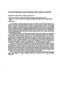
exponents γout between 2.1 and 2.7 and γin = 2.1 [9, 85, 81, 4, 3]. Several studies indicate that the WWW has small-world property. Albert et al. [9] shows that for a sample of around 320,000 nodes the average path length is 11.2 predicting an average path length of 19 for the full WWW (Fig. 1.1). Another study by Broder et al. [28] found that for a 50 million sample size the average path length is 16, in agreement with the predictions of Ref. [9]. 1.2.3 Metabolic Networks The metabolism in the cell can be represented as a directed network, the nodes being the substrates and the links the chemical reactions in which the substrates participate. Jeong et al. [75] analyzed the metabolism of 43 organisms and found that is has a small average path length and that the distribution of in- and outdegree follows a power law with degree exponent between 2.0 and 2.4 ( Fig. 1.2). Another study by Wagner and Fell [139] studying the Escherichia coli bacterium found that the undirected version of the network has a large clustering coefficient. 1.2.4 Genetic Regulatory Networks The network made of genes as nodes and genetic regulatory interactions as links is the genetic regulatory network. The reconstruction of the regulatory network in E. coli and S. cerevisiae show a scale-free topology and high clustering coefficient [102, 130]. 1.2.5 The Movie Actor Network The movie actor network is based on The Internet Movie Database (www.imdb.com), which is a continuously growing database containing movies with their casts since 1980. In the movie actor network the nodes are the actors and the links are between the actors acting together in a movie [142, 114]. The degree distribution of the

5

Figure 1.1. The distribution of the outgoing (a) and incoming (b) number of links of the nd.edu domain, containing 325, 729 documents and 1, 469, 680 links. The tail of the distributions follow power-law with exponents γout = 2.45 ans γin = 2.1. (c) The average shortest path between two documents as a function of the system size. The inset shows the universal feature of the www, the slopes being the same for different starting points of the measurement [9].

6

Figure 1.2. The degree distribution of the metabolic network, showing separately the number of outgoing and the number of incoming links: (a) A. fulgidus; (b) E. coli; (c) C. elegans. The distribution of in- and out-degree follows a power law with degree exponent between 2.0 and 2.4 [75].

7

actor network has a power-law tail [18, 13, 6], with exponent 2.3 (Fig. 1.3) and a large clustering coefficient. 1.2.6 The Web of Human Sexual Contacts Liljeros et al. [89] analyzed the data gathered in 1999 in a Swedish survey about the sexual behavior of individuals. They studied the network constructed from the sexual relations of 2810 individuals (Fig. 1.4). They analyzed the distribution of partners over a single year, finding that for both man and woman it follows a power law degree distribution with exponents between 3 and 3.5. The scale-free nature of the sex-web was confirmed later by other studies [128]. 1.2.7 Email Networks In the email network the nodes are the email addresses and links are the emails. In the study by Ebel et al. [47] an email network was constructed from the log files of the email server at Kiel University over a period of 112 days, resulting in a network of 59, 812 nodes. The network has a small-world property and the degree distribution follows a power-law with exponent γ = 1.81 (Fig. 1.5) with exponential cutoff. 1.2.8 Phone Call Networks The phone calls made by individuals can be mapped as a directed network, the nodes being the individuals and the phone calls between them represented by links. A study by Aiello et al. [5] shows that the network constructed by the phone calls made during a single day follow a power law degree distribution for the outgoing and incoming calls with exponent 2.1 (Fig. 1.6).

8

k Figure 1.3. The degree distribution of the movie actor collaboration network. The size of the network is around 200, 000 and the exponent of the degree distribution is γ = 2.3 [18].

9

1.2.9 Protein-Interaction Networks One of the important cellular networks is the protein-interaction network, where the nodes are the proteins and the links are the physical interactions between them (Fig. 1.7). Recent studies show that for S. cerevisiae, H. pylori, C.elegans and D. melenogaster the protein interaction network follows a power-law [74, 138, 125, 55]. 1.2.10 Citation Networks The citation network consist of the citation pattern of scientific publications, the nodes being the articles and the directed links representing a citation to a previous article. Studies on citation networks show that the in-degree distribution follows a power-law (Fig. 1.8) with exponent 3 [124, 126, 129, 127] and the out-degree distribution has an exponential tail [137]. 1.2.11 Collaboration Networks In the collaboration network, the nodes consist of scientists and the links are between scientists who have written an article together. Newman studied four databases over a five-year time period [109, 107, 108]. All networks show small average path length and high clustering coefficient. Barab´asi et al. [20] also studied the collaboration network of mathematicians and neuroscientists finding a small average path length, high clustering coefficient, and power-law degree distributions (Fig. 1.9). 1.2.12 Neural Networks In the neural network the nodes are the neurons and the links are neurons if they are connected by a synapses or a gap junction. The worm C. elegans has 282 neurons [143]. This small network has an exponential degree distribution and high clustering coefficient [142, 13].

10

1.2.13 Ecological Networks In food webs, the nodes are the species and the links represent the predator-prey relationship between them. Studies on food webs indicate that they are highly clustered and have small a world-property [144, 103, 30]. The nature of their degree distribution is unclear, some studies found a power-law [103], others exponential behavior [30, 31].

11

Figure 1.4. (a) Distribution of number of partners of individuals in 12 months [89]. The distributions are power-law, for females γ = 2.5 and for males γ = 2.31. (b) Distribution of the total number of partners over an entire lifetime. For females γ = 2.1 and for males γ = 1.6.

12

Figure 1.5. The degree distribution of an email network constructed from the log files of the email server at Kiel University over a period of 112 days [47]. The distribution follows a power-law with exponent γ = 1.81.

13

Figure 1.6. The distribution of out- and in-degree of a phone call network follows a power-law with exponents 2.1 [5].

14

(a)

(b)

Figure 1.7. (a) The protein interaction network in yeast. (b) The degree distribution of the protein interaction network in yeast follows a power-law with exponential cutoff, P (k) ∼ (k + k0 )−γ exp(−(k + k0 )/kc ), with k0 ≈ 1, kc ≈ 20 and γ = 2.4 [74].

15

Figure 1.8. The citation distribution from the Institute of Scientific Information (triangle) and Physical Review D (circle) dataset. The straight line represents a slope of −3 [126].

16

Figure 1.9. The degree distribution for mathematics (a) and neuroscience (b) journals. (c) Degree distribution shown with logarithmic binning, the lines corresponding to the best fits with slopes 2.1 (neuroscience) and 2.4 (mathematics) [20].

17

CHAPTER 2 MODELING NETWORKS

In this chapter we present the most important network models developed to describe the topological properties of complex networks. First we present the random network introduced by Erd˝os and R´enyi (ER model). After discussing several important topological properties of the Erd˝os-R´enyi model, we introduce the network model proposed by Barab´asi and Albert, the first model being able to describe the powerlaw degree distribution of real networks and also giving insight into the organization principles governing the growth of real networks. 2.1 The Erd˝ os-R´enyi Model The theory of random graphs was introduced by Erd˝os and R´enyi [49]. In their model they start with N nodes and connect each node pair with probability p (Fig. 2.1), thus the model for p = 1 results in a fully connected graph. At p = pc ≈ 1/N the random graph changes its topology from a group of smaller clusters to a system which is dominated by a giant cluster [24]. The largest clusters’s size S increases proportionally with the separation from the critical probability: S ∼ (p − pc )

(2.1)

The average degree of the network is given by: < k >= p(N − 1) ≈ pN

18

(2.2)

(a)

(b)

Figure 2.1. (a) In the ER model each node pair is connected with the same p probability, all nodes having similar number of links. (b) The degree distribution of ER model follows a Poisson degree distribution chatacterized by a well defined average (< k >) degree.

19

2.1.1 Degree Distribution The probability that a node has k links in the ER model follows a binomial distribution. The probability that a node has k links is pk and the probability of not having the possible N − k − 1 links is (1 − p)(N −k−1) . Including all the possible ways k links can be placed (CNk −1 ) the degree distribution becomes P (k) = CNk −1 pk (1 − p)N −k−1 ,

(2.3)

which for large N converges to the Poisson distribution P (k) ≈ e−pN

(pN )k k!

(2.4)

Despite the fact that the links are placed randomly, a random graph is rather homogeneous, most of the nodes having the same number of edges. 2.1.2 The Average Path Length Random graphs have small average path length if p is not too small. The reason is that because of a homogeneous degree distribution the number of nodes at a distance l can be approximated as < k >l . From N =< k >l , the average path lenght of a random network scales as: l≈

ln(N ) ln(< k >)

(2.5)

The average path length of many real networks is close to the average path length of random graphs with the same size [7]. 2.1.3 Clustering Coefficient In a random graph if we consider a node, its neighbors are connected with probability p leading to: C=p= 20

. N

(2.6)

The clustering coefficient for most real networks is much higher than the one for the ER model [7]. 2.2

The Barab´ asi-Albert Model

The origin of the power-law degree distribution was first addressed by Barab´asi and Albert [18]. They show that the scale-free nature of real networks is rooted in two basic ingredients: growth and preferential attachment. Most complex networks like the world wide web or citation networks are characterized by continuous growth through the addition of new web sites or publications. The preferential attachment in these examples has its origin in the fact that the new pages are more likely to include hyperlinks to already well connected web pages and the new papers also tend to cite already well cited papers. The model introduced by Barab´asi and Albert has the following ingredients: • Growth: we start with m0 number of nodes and at every time step we add a new node with m edges to the network. • Preferential attachment: the probability Π that a new node will be connected to a node ”i” depends on the connectivity ki of that node:

ki Π(ki ) = P j

kj

(2.7)

After time t, this procedure results in a network with N = t + m0 nodes and mt edges (Fig. 2.2). 2.2.1 Degree Distribution There are various analytical approaches to calculate the degree distribution of the BA model. The first proposed by Barab´asi et al. [19] focuses on the time evolution of

21

a node’s degree. This was followed by the master-equation approach by Dorogovtsev et al. [45] and the rate equation introduced by Krapivsky et al. [83]. The exact solution of the degree distribution was provided by Bollob´as et al. [26]. The continuum approach [19] first calculates the time dependence of the degree of a given node. Approximating ki as a continuous variable, the rate of increase in the degree is proportional to Π(ki ): ∂ki ki = m Π(ki ) = m PN −1 , ∂t j=1 kj P −1 where the sum in the denominator can be written as: N j=1 kj = 2mt, thus ∂ki ki = . ∂t 2t

(2.8)

(2.9)

The initial condition of this equation is that each node i is introduced at time ti leading to

r t . ki (t) = m ti

(2.10)

The probability that a node has a degree ki (t) < k is given by: µ P (ki (t) < k) = P

m2 t ti > 2 k

¶ .

(2.11)

The probability that a node was added to the system at the time ti is P (ti ) =

1 , m0 + t

(2.12)

thus the probability P (m2 t/k 2 ) is given by: µ P

m2 t ti > 2 k

¶ =1−

m2 t . k 2 (m0 + t)

(2.13)

The degree distribution P (k) can be obtained from equation (2.13) P (k) =

2m2 t 1 . m0 + t k 3 22

(2.14)

The effects of nonlinear Π(k) was studied by Krapivsky et al. [84], showing that the topology of the network is scale-free only for linear preferential attachment, the sublinear attachment resulting in a stretch exponential and the superlinear attachment resulting in the ”winner-takes-all” phenomena, all nodes connecting to the same node only. 2.2.2 Average Path Length The average path length is smaller for the BA model than the corresponding random network. Analytical results show that for scale-free networks [27, 38, 34] are “ultrasmall” the average path length scaling as: l ∼ ln(ln N ).

(2.15)

These results hold for any scale-free network with degree exponent between 2 and 3. 2.2.3 Clustering Coefficient The clustering coefficient was calculated analytically for the BA model and it is given by [82, 25]:

C∼

(ln N )2 . N

(2.16)

In the first two chapter we presented the properties of many real networks and two of the most influential network models. In the following chapter we will present a simple epidemic model and show that one of the consequences of the scale-free nature of real networks is the vanishing epidemic threshold. Finally, we discuss immunization strategies targeting the hubs to stop an epidemic on a scale-free network.

23

(a)

(b)

Figure 2.2. (a) In the BA model at every timestep a new node connects to already well connected nodes (red links). (b) The degree distribution of the BA model in a log-log plot, following a power-law degree distribution with exponent 3.

24

CHAPTER 3 EPIDEMIC SPREADING ON NETWORKS

Many of the diffusion processes of practical interest, ranging from the spread of computer viruses to the diffusion of sexually transmitted diseases, take place on complex networks. Biological viruses spread on the network defined by the connection between individuals, such as the web of sexual connections responsible for the spread of the HIV virus or the human-contact network responsible for the spread of viruses like SARS. The spread of computer viruses also can be described in the context of networks, some computer viruses being attached to emails and spreading through the email network. Understanding the topological properties of networks responsible for the spread of diseases helps to design efficient immunization strategies to stop epidemics. In biological networks the immunization consist in the administration of cures to the population, while in the computer world the immunization comes in form of an antivirus software. While classical epidemiological models consider viruses propagating on regular lattices or random networks with homogeneous degree distributions [43, 15], the real networks responsible for virus spreading are scale-free. In this chapter we show the general framework for epidemic modeling in complex networks and how the topological properties of networks impact on the spreading process. We investigate immunization strategies for scale-free networks, the real networks responsible for the spread of viruses being characterized by a scale-free topology [47, 89].

25

3.1 Modeling Epidemics in Networks In the statistical modeling of epidemics a quantity often studied is the density of infected nodes. The individuals can exist in a discrete set of states such as susceptible (healthy), infected, immune and dead (removed). The population in which the epidemic propagates can be described as a network, where vertices represent the individuals and the edges are the connection along which the virus spreads. The simplest model of epidemic spreading is the susceptible-infected-susceptible (SIS) model [43, 15]. In this model an individual is represented by a node, which can be either ”healthy” or ”infected”. Connections between individuals along which the infection can spread are represented by links. In each time step a healthy node is infected with probability ν if it is connected to at least one infected node. At the same time an infected node is cured with probability δ, defining an effective spreading rate λ ≡

ν δ

for the virus. Another model often used for modeling epidemics

is the susceptible-infected-removed (SIR) model, where the possibility of removing individuals from the population is included [43, 15, 106]. 3.1.1 Epidemics Spreading in Homogeneous Networks The behavior of the SIS model is well understood in random networks or regular lattices [43, 15, 106]. Studies indicate that the viruses whose spreading rate exceeds a critical threshold will persist, while those under the threshold will die out. In the following we study the dynamic rate equation for the density of infected nodes in a homogeneous network, characterized by small degree fluctuations. In the meanfield approximation, assuming that the correlation among the state of vertices are neglected, the fraction of infected nodes (ρ(t)) can be written as: dρ(t) = −δρ(t) + ν < k > ρ(t)[1 − ρ(t)]. dt 26

(3.1)

The first term on the right hand side represents infected individuals recovering with probability δ. The second term represents the rate of nodes being infected, being proportional with the infection probability ν, the density of healthy vertices (1−ρ(t)), and the number of infected individuals in contact with any healthy vertex, approximated as kρ(t). We considered that each vertex has the same number of edges, k ≈< k >. After imposing the stationary condition

dρ(t) dt

= 0 we obtain the

equation ρ[−1 + λ < k > (1 − ρ)] = 0.

(3.2)

The above equation predicts the existence of an epidemic threshold: λc =

1 .

(3.3)

If λ is above the threshold, λ > λc , the infection spreads and becomes an epidemic. Below the threshold λ < λc , the infection dies out (Fig. 3.1). 3.1.2 Epidemics Spreading in Scale-free Networks To take into account the degree fluctuations in the analytical description of the SIS model, we denote by ρk (t) the density of infected nodes with connectivity k, the time evolution of ρk (t) becoming [119]: ∂t ρk (t) = −δρk (t) + ν(1 − ρk (t))kθ(λ).

(3.4)

Equation (3.4) predicts that the epidemic threshold is:

λc =

. < k2 >

(3.5)

For scale-free networks for which the degree distribution follows a power-law with exponent γ ≤ 3, the variance of the degree distribution is infinite (< k 2 >→ ∞), therefore the epidemic threshold is zero. The vanishing epidemic threshold in scalefree networks is not just a property of the SIS model, but it was reproduced also 27

ρ(λ)

λc

λ

Figure 3.1. The epidemic threshold in homogeneous networks is finite. The epidemic below the epidemic threshold dies out.

28

in other epidemic models and appears to be a general property of heterogenous networks [104, 112, 94]. The finding that the epidemic threshold vanishes in scale-free networks has a strong impact on our ability to control various virus outbreaks. Indeed, most methods designed to eradicate viruses – biological or computer based – aim at reducing the spreading rate of the virus, hoping that if λ falls under the critical threshold λc , the virus will die out naturally. With a zero threshold, while a reduced spreading rate will decrease the virus’ prevalence, there is little guarantee that it will eradicate it. Therefore, from a theoretical perspective viruses spreading on a scale-free network appear unstoppable. The question is, can we take advantage of the increased knowledge accumulated in the past few years about network topology to understand the conditions in which one can successfully eradicate viruses? 3.2

Immunization in Scale-free Networks

3.2.1 Curing the hubs To restore a finite epidemic threshold, which would allow the infection to die out, one needs to induce a finite variance (3.5). As the origin of the infinite variance is in the tail of the degree distribution, dominated by the hubs, one expects that curing all hubs with degree larger than a given degree k0 would restore a finite variance and therefore a nonzero epidemic threshold. Indeed, studies [91, 94] indicate that if on a scale-free network nodes with degree k > k0 are always healthy, the epidemic threshold is finite and has the value: µ ¶−1 k0 − m k0 = . λc = ln < k2 > k0 m m

(3.6)

This expression indicates that the more hubs we cure (i.e. the smaller k0 is), the larger the value of the epidemic threshold (Fig. 3.2).

29

0.8

λC

0.6

0.4

0.2

0

50

100

k0 Figure 3.2. The epidemic threshold as a function of k0 . On a scale-free network if we cure all nodes with degree k > k0 the epidemic threshold becomes finite.

30

3.2.2 Targeting the Hubs In many complex networks responsible for disease spreading the problem is that we we do not have detailed network maps, thus we cannot effectively identify the hubs. Indeed, we do not know the number of sexual partners for each individual in the society, thus we cannot identify the social hubs that should be cured if infected. Similarly, on the email network we do not know which email accounts serve as hubs, as these are the ones that, for the benefit of all email users, should always carry the latest anti-virus software. Short of a detailed network map, no method aiming to identify and cure the hubs is expected to succeed at its goal of finding all hubs with degree larger than a given k0 . Yet, policies designed to eradicate viruses could attempt to identify and cure as many hubs as possible. Such biased policy will inevitably be inherently imperfect, as it might miss some hubs, and falsely identify some smaller nodes as hubs. In the following we will study policies biased towards curing the hubs, incorporating in our model our limited ability of identifying and curing the hubs. Numerical Results To investigate the effect of incomplete information about the hubs we assume that the likelihood of identifying and administering a cure to an infected node with k links in a given time frame depends on the node’s degree as k α , where α characterizes the policy’s ability to identify hubs [40]. In this framework α = 0 corresponds to random cure distribution, which is expected to have zero epidemic threshold while α = ∞ corresponds to an optimal policy that treats all hubs with degree larger than k0 . Within the framework of the SIS model we assume that each node is infected with probability ν, but each infected node is cured with probability δ = δ0 k α , becoming again susceptible to the disease. We define the spreading rate as λ =

31

ν . δ0

As each

healthy node is susceptible again to the disease, a node can get multiple cures during a simulation. We place the nodes on a scale-free network and initially infect half of them. After a transient regime the system reaches a steady state, characterized by a constant average density of infected nodes, ρ, which depends on both the spreading rate λ and α (Fig. 3.3). The α = 0 limit corresponds to random immunization in which case the epidemic threshold is zero. As treating only the hubs will restore the nonzero epidemic threshold, for α = ∞ we expect a nonzero λc . Yet, the numerical simulations indicate that we have a finite λc well before the α = ∞ limit. Indeed, as figure 3.3 shows, λc is clearly finite for α = 1 and so is for smaller value of α as well. The numerical simulations do not give an unambiguous answer the crucial question: Is there a critical value of α at which a finite λc appears, or for any any nonzero α we have a finite λc ? Mean-field theory To interpret the results of the numerical simulations we studied the effect of a biased policy using the mean-field continuum approach [119]. Denoting by ρk (t) the density of infected nodes with connectivity k, the time evolution of ρk (t) can be written as ∂t ρk (t) = −δ0 k α ρk (t) + ν(1 − ρk (t))kθ(λ).

(3.7)

The first term in the r.h.s. describes the probability that an infected node is cured, and it is therefore proportional to the number of infected nodes ρk (t) and the probability δ0 k α that a node with k links will be selected for a cure. The second term is the probability that a healthy node with k links is infected, proportional to the infection rate (ν), the number of links (k), the number of healthy nodes with k links (1 − ρk (t)), and the probability θ(λ) that a given link points to an infected node.

32

0.8

ρ

0.6

0.4

0.2

0

0

0.5

1

λ

1.5

2

Figure 3.3. Prevalence, ρ, measured as the fraction of infected nodes in function of the effective spreading rate λ for α = 0(o), 0.25(¤), 0.50(∇), 0.75(♦) and 1(4), as predicted by Monte-Carlo simulations using the SIS model on a scale-free network with N=10,000 nodes.

33

The probability θ(λ) is proportional to kP (k), therefore it can be written as θ(λ) = Using λ =

ν δ0

X kP (k) P ρk . sP (s) s k

(3.8)

and imposing the ∂t ρk (t) = 0 stationary condition we find the station-

ary density as ρk =

λθ(λ) . k α−1 + λθ(λ)

(3.9)

Combining equations (3.8) and (3.9) and using the fact that the connectivity distribution P (k) = 2m2 /k −3 for the scale-free network, we obtain: Z ∞ dk mλ = 1. 2 α−1 + λθ(λ)) m k (k The average density of infected nodes is given by Z ∞ X 2 P (k)ρ(k) = 2m λθ(λ) ρ(λ) = m

k

dk + λθ(λ))

k 3 (k α−1

(3.10)

(3.11)

Equations 3.10 and 3.11 allow us to calculate the average density of infected nodes for any value of α. For α = 0 they reduce to the case studied in Ref. [120] giving λc = 0. For α = 1 we can solve (3.10), and using (3.11) we obtain ρ(λ)|α=1 =

λ−1 , λ

(3.12)

which indicates that for α = 1 the epidemic threshold is finite, having the value λc (α = 1) = 1 [120]. To determine the epidemic threshold as a function of α we need to solve the ρ(λ) = 0 equation. While we cannot get ρ(λ) for arbitrary values of α, we can solve equation (3.10) in λ using that at the threshold λ = λc we have θ(λc ) = 0. In this case (3.10) predicts that the epidemic threshold depends on α as λc = αmα−1 .

(3.13)

For α = 0 we recover λc = 0, confirming that random immunization cannot eradicate an infectious disease. For α = 1 equation (3.13) predicts that the epidemic threshold 34

1 0.8

λc

0.6 0.4 0.2 0

0

0.2

0.4

α

0.6

0.8

1

Figure 3.4. The dependence of the epidemic threshold λc on α as predicted by our calculations (continuous line) based on the continuum approach, and by the numerical simulations based on the SIS model (boxes). The small deviation between the numerical results and the analytical prediction is due to the uncertainty in determining the precise value of the threshold in Monte-Carlo simulations.

35

is λc = 1, in agreement with (3.12). Most important, however, equation (3.13) indicates that λc is nonzero for any positive α, i.e., any policy that is biased towards curing the hubs can restore a finite epidemic threshold. Furthermore, policies with larger α are expected to be more likely to lead to the eradication of the virus, as they result in larger λc values. Therefore, equation (3.13) indicates that a potential avenue to eradicating a virus is to increase the effectiveness of identifying and curing the hubs. Indeed, if the virus has a fixed spreading rate, increasing α could increase λc beyond λ, thus making possible for the virus to die out naturally. To test the validity of prediction (3.13) we determined numerically the λ(α) curve from the simulations shown in figure 3.4). As figure (3.4) shows, we find excellent agreement between the simulations and the analytical prediction (3.13). Cost-effectiveness: An important criteria for any policy designed to combat an epidemic is its costeffectiveness. Supplying cures to all nodes infected by a virus is often prohibitively expensive. Therefore, policies that obtain the largest effect with the smallest number of administered cures are more desirable. To address the cost-effectiveness of a policy targeting the hubs we calculated the number of cures administered in a time step per node for different values of α. Figure (3.5) indicates that increasing the policy’s bias towards the hubs by allowing a higher value for α decreases rapidly the number of necessarily cures. Therefore, policies that distribute the cures mainly to the nodes with more links are more cost effective than those that spread the cures randomly, blind to the node’s connectivity. We can understand the origin of the rapid decay in c(α) by noticing that the number of cures administered per unit time is proportional to the density of infected nodes.

36

0.4

c

0.3

0.2

0.1

0

0

0.2

0.4

α

0.6

0.8

1

Figure 3.5. The number of cures, c, administered in an unit time per node for different values of α. The rapidly decaying c indicates that more successful is a policy in selecting and curing hubs (larger is α), fewer cures are required for a fixed spreading rate (λ = 0.75). For α = 0 the number of cures is calculated by c = ν/(ν + δ) = λ/(1 + λ) which gives c = 0.43, which value is in good agreement with the numerical results.

37

3.2.3 Conclusions One of the very important consequences of the scale-free nature of real networks is the vanishing epidemic threshold. Our numerical an analytical results indicate that targeting the more connected infected nodes can restore the epidemic threshold, therefore making possible the eradication of a virus. Most important, however is the finding that even not very successful policies with small α values can lead to a nonzero epidemic threshold. As the magnitude of λc rapidly decreases with α, the more effective a policy is at identifying and curing the hubs of a scale-free network, the higher are its chances of eradicating the virus. Our numerical results are supported by analytical calculations. Finally, the simulations shows that a biased treatment policy is not only more efficient but it is also less expensive than random immunization. These results, beyond improving our understanding of the basic mechanism of virus spreading, could also offer important input into designing effective policies to eradicate computer or biological infections.

38

CHAPTER 4 THE DYNAMICS OF INFORMATION ACCESS ON THE WORLD WIDE WEB

The world wide web is a virtual network on the Internet, whose nodes are the Web pages and the links are the hyperlinks pointing from one page to another. The WWW is an example of an evolving network, new Web pages and links appearing and disappearing at a very fast rate. The complexity of the WWW consists of its complex structure, the rapid evolution in time of the structure and the various dynamics taking place on it, such as the browsing dynamics of the users. In this chapter we present some of the studies aiming to describe the topology of the Web and a series of network models that reproduce some of the WWW’s topological features. Finally, we study a large news portal as a model system of a rapidly changing and evolving network. First we study the structure of the web portal, then we focus on the interplay between network dynamics and the visitation history of individual documents. 4.1

The Topological Characteristics of the WWW

4.1.1 The Structure of the Web The experiments aimed to study the structure of the WWW are based on Web crawlers, which explore the topology by following the links found on each page. The Web is a directed network and generally is much more difficult to determine the in-degree distribution.

39

The first study of the Web was proposed by Albert et al. [9] in a study where the authors analyzed the data collected by a Web crawler which mapped the Web pages and hyperlinks in University of Notre Dame. This analysis showed that the that Web has a small-world character characterized by an average shortest path of < l >= 11. The authors also measured the in- and out-degree distribution of the Web, showing that it follows a power-law with exponents γin = 2.4 and γout = 2.1. This work was followed by further studies of larger samples of the WWW [28, 85]. A study by Broder et al. [28] identified the complex hierarchy of connected components of the WWW. The study shows that the Web consists of a giant strongly connected component (56 millions pages), which is characterized by direct paths between any pair of pages. Connected to this component are the IN and OUT components (44 millions of pages each) (Fig. 4.1). These sets are formed by pages linked by directed paths that either enter or exit the giant component. Therefore, from any node in the IN component is possible to reach the OUT component by passing through nodes in the giant component. There is no path, however, from the OUT component going back to the giant component. There are also tendrils and disconnected islands, that are unreachable from the giant component, which can contain thousands of Web documents. The existence of these components are a consequence of the directed nature of the WWW and significantly limit the Web’s navigability. The existence of the giant component, the IN and OUT components is a property of all directed networks. This was demonstrated recently by Dorogovstev et al. [46], showing that the size and structure of the components can be predicted analytically. Another feature of the WWW is the existence of a large number of communities, the high clustering coefficient confirming the clustered nature of the WWW [86, 85, 51, 81].

40

Figure 4.1. The structure of the Web. The study shows that the Web consists of a giant strongly connected component (56 millions pages), which is characterized by direct paths between any pair of pages. Connected to this component are the IN and OUT components (44 millions of pages each). These sets are formed by pages linked by directed paths that either enter or exit the giant component. There are also tendrils and disconnected islands, that are unreachable from the giant component [28].

41

4.1.2 Modeling the WWW The Web models have two basic ingredients: the continuous growth of the network by adding new nodes and the preferential attachment mechanism, which consist in the fact that the new nodes are being attached preferentially to nodes with high degree. The first model of the WWW was proposed by Drogovtsev et al. [46]. In this model at each time step a new node is introduced and connected with probability Π(kin ) ∼ A + kin to m number of already existing nodes, where A is a constant and determines the attractiveness of each node. The in-degree distribution of the network constructed by this algorithm has the form P (kin ) ∼ (A + kin )(−2−A/m) . The degree exponent can be tuned by changing the parameter A. The out-degree distribution is a delta function, P (kout ) = δ(kout − m). A model with similar structure was proposed by Pennock et al. [122]. In this model both endpoints of a links are chosen according to a probability of α for preferential attachment and 1 − α for uniform attachment. This model accurately accounts for the connectivity distributions of category-specific web pages and the web as a whole. Other studies take into account the fact that links between pairs of nodes change on a very short time scale. Krapivsky, Rodgers, and Redner [84] developed models of the WWW in which they included the rewiring of links. In this model a new node is introduced with probability p and attached to a node already present in the network, the attachment probability depending on the in-degree of the target. With probability 1 − p a new link is created between already existing nodes, depending on the out-degree of the originating node and the in-degree of the target. This process generates correlated in-degree and out-degree distributions. The copying mechanism is an alternative mechanism for preferential attachment in the study by Kleinberg [81]. The idea behind the copying mechanism is that new pages dedicated to a certain thematic area 42

copy hyperlinks from already existing pages with similar contents. In this model at each time step a new node is added to the network and a node is selected randomly from those already present in the network. The new node has m outgoing links connected to the nodes to which the randomly selected node points. With probability α the links are rewired on randomly selected nodes and with probability 1 − α the links remain unchanged. In this model the out-degree is by construction −(2−α)/(1−α)

P (k) = δ(kout − m) and the in-degree is a power law, P (k) ∼ kin

, thus α

being the tuning parameter for the degree exponent and also controlling the number of cliques formed by the network. Other models include the combination of preferential attachment with the fact that websites with similar contents are more likely to be connected [98] and other studies relate the topology of the WWW with the relative growth rate of nodes and links [68]. 4.2

The Visitation Dynamics of a Web Portal

While most of the studies on complex networks focus on systems that change relatively slowly in time, the structure of the Web is altered at the time scale from hours to to days. The most visited portion of the WWW, ranging from news portals to commercial sites change within hours through the rapid addition and removal of documents and links. We investigate the dynamics of visitation of a major news portal [42], representing the prototype of such a rapidly evolving network. This is driven by the fleeting quality of news: in contrast with the 24-hour news cycle of the printed press, in the online media the non-stop stream of new developments often obliterates an event within hours. But the WWW is not the only rapidly evolving network: the wiring of a cell’s regulatory network can also change very rapidly during cell cycle or when there are rapid changes in environmental and stress factors [115]. Similarly, while in social networks the cumulative number of friends and ac-

43

quaintances an individual has is relatively stable, an individual’s contact network, representing those that it interacts with during a given time interval, is often significantly altered from one day to the other. Given the widespread occurrence of these rapidly changing networks, it is important to understand their topology and dynamical features. 4.2.1 Description of the Data Automatically assigned cookies allow us to reconstruct the browsing history of approximately 250,000 unique visitors of the largest Hungarian news and entertainment portal (origo.hu), which provides online news and magazines, community pages, software downloads, free email and search engine, capturing 40% of all internal Web traffic in Hungary. The portal receives 6,500,000 HTML hits on a typical workday. We used the log files of the portal to collect the visitation pattern of each visitor between 11/08/02 and 12/08/02, the number of new news documents released in this time period being 3,908. The prime data sources are the web server log files, containing all HTML requests. A hit has standard attributes like client host, request time, request code, http request (containing the page url), referee, agent identification string, and contains session identification cookie as well. 4.2.2 The Structure of the Web Portal From a network perspective most web portals consist of a stable skeleton, representing the overall organization of the web portal, and a large number of news items that are documents only temporally linked to the skeleton. Each news item represents a particular web document with a unique URL. A typical news item is added to the main page, as well as to the specific news subcategories to which it belongs. For example, the report about an important soccer match could start out simultaneously on the front page, the sports page and the soccer subdirectory of the sports 44

page. As a news document “ages”, new developments compete for space, thus the document is gradually removed from the main page, then from the sports page and eventually from the soccer page as well. After some time (which varies from document to document) an older news document, while still available on the portal, will be disconnected from the skeleton, and can be accessed only through a search engine. To fully understand the dynamics of this network, we need to distinguish between the stable skeleton and the news documents with heavily time dependent visitation. The documents belonging to the skeleton are characterized by an approximately constant daily visitation pattern, thus the cumulative number of visitors accessing them increases linearly in time. In contrast, the visitation of news documents is the highest right after their release and decreases in time, thus their cumulative visitation reaches a saturation after several days. This is illustrated in figure (4.2), where we show the cumulative visitation for the main page (www.origo.hu/index.html) and a typical news item. The difference between the two visitation patterns allows us to distinguish in an automated fashion the websites belonging to the skeleton from the news documents. For this we make a linear regression to each site’s cumulative visitation pattern and calculate the deviation from the fitted lines, documents with very small deviations being assigned to the skeleton. The validity of the algorithm was checked by inspecting the URL of randomly selected documents, as the skeleton and the news documents in most cases have a different format. But given some ambiguities in the naming system, we used the visitation-based distinction to finalize the classification of the documents into skeleton and news. When visiting a news portal, we often get the impression that it has a hierarchical structure. As shown in figure 4.3 the skeleton forms a complex network, driving the

45

6e+06

12000

(a)

(b) 10000

4e+06

8000 6000

2e+06

4000 2000

0

0

1000 2000 3 Time (10 s)

3000 0

0 500 1000 1500 2000 3 Time (10 s)

Figure 4.2. The cumulative number of visits to a typical skeleton document (a) and a news document (b). The difference between the two visitation patterns allows us to distinguish between news documents and the stable documents belonging to the skeleton.

46

visitation patterns of the users. Indeed, the main site, shown in the center, is the most visited, and the documents to which it directly links to also represent highly visited sites. In general (with a few notable exceptions, however), the further we go from the main site on the network, the smaller is the visitation. The skeleton of the studied portal has 933 documents with an average degree close to 2 (i.e. it is largely a tree, with only a few loops, confirming our impression of a hierarchical topology), the network having a few well connected nodes (or hubs), while many are linked to the skeleton by a single link [18, 19]. 4.2.3 The Characteristics of News Item Visitation From the HTML hits we can measure the number of hits or visits a particular news item receives. The number of news released in one month time period is 3,908. We shift the release day of the news items to the same day and average over the visitation pattern. The release day in our study corresponds to the day of the first visit of a particular new item (4.4a). In order to find the functional form of the visitation decay we have to eliminate the periodic daily fluctuation in the number of visitors. We achieve this by redefining the time unit as one web page request on the portal (4.4b). After performing logarithmic binning we found that the decay of the visitation follows a power-law (n(t) ∼ (t + t0 )−β ), with t0 = 12 and β = 0.3 ± 0.1 (4.4c). The overall visitation of a specific document is expected to be determined both by the document’s position on the web page, as well as the content’s potential importance for various user groups. In general the number of visits n(t) to a news document follows a dampened periodic pattern: the majority of visits (28%) take place within the first day, decaying to only 7% on the second day, and reaching a small but apparently constant visitation beyond four days (Fig. 4.4a). Further, we want to characterize a news item by the interest it generates, which

47

Figure 4.3. The skeleton of the studied web portal has 933 nodes. The area of the circles assigned to each node in the figure is proportional with the logarithm of the total number of visits to the corresponding web document. The width of the links are proportional with the logarithm of the total number of times the hyperlink was used by the surfers on the portal. The central largest node corresponds to the main page (www.origo.hu/index.html) directly connected to several other highly visited sites.

48

Visitation

60

(a)

40 20 0

0

5

1

8 Visitation

10

Time (days)

10

(c)

(b)

6 4 2 0

0

0

10

0

1

2

3

4

5

10 20 30 40 50 10 10 10 10 10 10 3

5

Time(10 units)

Time (10 units)

Figure 4.4. (a) The visitation pattern of news documents on a web portal. The data represents an average over 3,908 news documents, the release time of each being shifted to day one, keeping the release hour unchanged. The first peak indicates that most visits take place on the release day, rapidly decaying afterward. (b) The same as plot (a), but to reduce the daily fluctuations we define the time unit as one web page request on the portal. (c) Logarithmic binned decay of visitation of (b) shown in a log-log plot, indicating that the visitation follows n(t) ∼ (t + t0 )−β , with t0 = 12 and β = 0.3 ± 0.1 shown as a continuous line on both (b) and (c).

49

is a function of the total number of visits it receives and also the time frame in which receives all these visits. It is useful to characterize the interest in a news document by its half-time (T1/2 ), corresponding to the time frame during which half of all visitors that eventually access it have visited. We find that the overall half-time distribution follows a power law (Fig. 4.5), indicating that while most news have a very short lifetime, a few continue to be accessed well beyond their initial release. The average half-time of a news document is 36 hours, i.e. after a day and a half the interest in most news fades. A similar broad distribution is observed when we inspect the total number of visits a news document receives (Fig. 4.6), indicating that the vast majority of news generate little interest, while a few are highly popular [98]. Similar weight distributions are observed in a wide range of complex networks [56, 57, 22, 133, 147]. 4.2.4 Waiting Time Distribution of Individual Users In the following we connect the visitation decay of news items with the visitation patterns of individual users. We characterize the visitation pattern of users by studying the time interval distribution between two consecutive visits. We found that for all users the time interval distribution between visits follows a power-law with exponent α = 1.2 (Fig 4.8). We also studied the exponent distribution of the individual users, the exponents being peaked around 1.1 (Fig. 4.7). This means that for each user numerous frequent downloads are followed by long periods of inactivity, a bursting, non-Poisson activity pattern that is a generic feature of human behavior [16] and it is observed in many natural and human driven dynamical processes [116, 2, 136, 39, 80, 121, 123, 97, 65, 61, 14, 72]. An interesting consequence of the short display time of a given news document, and the uneven visitation pattern of individual users is that many users could miss

50

3

10

2

10

1

10

0

10

−1

10

−2

10

1

10

2

10 3 T1/2 (10 s)

3

10

Figure 4.5. The half-time distribution for individual news items, following a powerlaw with exponent −1.5.

51

3

10

2

N(n vists)

10

1

10

0

10

2

3

10

10

n visits Figure 4.6. The distribution of the total number of visits different news documents receive during a month. The tail of the distribution follows a power law with exponent 1.5.

52

15000

N(αi)

10000

5000

0

−2

−1.5

−1

−0.5

0

αι

Figure 4.7. The distribution the exponents of time intervals distribution between two consecutive visits of an individual user.

53

5

10

3

P (τ)

10

1

10

−1

10

−3

10

−4

10

−2

10

0

10 3 τ (10 s)

2

10

4

10

Figure 4.8. The distribution of time intervals between two consecutive visits of all users. The cutoff for high τ (τ ≈ 106 ) captures finite-size effects, as time delays over a week are undercounted in the month-long data set. The continuous line has slope α = 1.2.

54

a significant fraction of the news by not visiting the portal when a document is displayed. We find that a typical user sees only 53% of all news items appearing on the main page of the portal, and downloads (reads) only 7% of them. Such shallow news penetration is likely common in all media, but hard to quantify in the absence of tools to track the reading patterns of individuals. In the next section we show that the uneven visitation pattern is responsible for the slow decay in the visitation of a news document and that n(t) can be derived from the browsing pattern of the individual users. 4.2.5 The Origin of the Power-law Decay in Visitation To understand the origin of the observed decay in visitation, we assume that the portal has N users, each reading the news document of direct interest for him/her. Therefore, at every time step each user reads a given document with probability p. Users will not read the same news more than once, therefore the number of users which have not read a given document decreases with time. We can calculate the time dependence of the number of potential readers to a news document using dN (t) = −N (t)p dt

(4.1)

where N (t) is the number of visitors which have not read the selected news document by time t. The probability that a new user reads the news document is given by N (t)p. Equation (4.1) predicts that N (t) = N exp(−t/t1/2 )

(4.2)

where t1/2 = 1/p, characterizing the halftime of the news item. The number of visits (n) in unit time is given by

n(t) = −

dN N = exp(−t/t1/2 ). dt t1/2 55

(4.3)

Our measurements indicate, however, that in contrast with this exponential prediction the visitation does not decay exponentially, but its asymptotic behavior is best approximated by a power law (4.4c). n(t) ∼ t−β

(4.4)

with β = 0.3 ± 0.1, so that while the bulk of the visits takes place at small t, a considerable number of visits are recorded well beyond the document’s release time. Next we show that the failure of the exponential model is rooted in the uneven browsing patterns of the individual users. Indeed, equation (4.1) is valid only if the users visit the site in regular fashion such that they all notice almost instantaneously a newly added news document. In contrast, we find that the time interval between consecutive HTML requests by the same visitor is not uniform, but follows a powerlaw distribution, P (τ ) ∼ τ −α , with α = 1.2 ± 0.1 (Fig. 4.8). Let us assume that a given news document was released at time t0 and that all users visiting the main page after the release read that news. Because each user reads each document only once, the visitation of a given document is determined by the number of new users visiting the page where the document is featured. In figure 4.9 we show the browsing pattern for four different users, each vertical line representing a separate visit to the main page. The thick lines show for each user the first time they visit the main page after the studied news document was released at t0 . The release time of the news (t0 ) divides the time interval τ into two consecutive visits of length t0 and t, where t + t0 = τ . The probability that a user visits at time t after the news was released is proportional to the number of possible τ intervals, which for a given t is proportional to the possible values of t0 given by the number of intervals having a length larger than t,

56

New news item

user 1 user 2 t’

t

user 3 τ user 4 t0 time

Figure 4.9. The browsing pattern of four users, every vertical line representing the time of a visit to the main page. The time a news document was released on the main page is shown at t0 . The thick vertical bars represent the first time the users visit the main page after the news document was released, i.e. the time they could first visit and read the article.

57

Z

∞

P (τ > t) =

τ −α dτ ∼ t−α+1 .

(4.5)

t

If we have N users, each following a similar browsing statistics, the number of new users visiting the main page and reading the news item in a unit time (n(t)) follows

n(t) ∼ N P (τ > t) ∼ N t−α+1 .

(4.6)

Equation (4.6) connects the exponent α characterizing the decay in the news visitation to β in equation (4.4), characterizing the visitation pattern of individual users, providing the relation β = α − 1.

(4.7)

This is in agreement with our measurements within the error bars, as we find that α = 1.2 ± 0.1 and β = 0.3 ± 0.1. To further test the validity of our predictions we studied the relationship between α and β for the more general case, when a user that visits the main page reads a news item with probability p. We numerically generated browsing patterns for 10,000 users, the distribution for the time intervals between two consecutive visits, P (τ ), following a power-law with exponent α = 1.5 (Fig. 4.10 inset). In figure 4.10 we calculate the visits for a given news item, assuming that the users visiting the main page read the news with probability p, characterizing the ”stickiness” or the potential interest in a news item. As we see in the figure the value of β is close to 0.5 as predicted by (4.6). Furthermore, we find that β is independent of p, indicating that the inter-event time distribution P (τ ) characterizing the individual browsing patterns is the main factor that determines the visitation decay of a news document, the difference in the content (stickiness) of the news playing

58

2

10

8

10 6 10 4 10 2 10 0 10

1

Number of visits

10

10

β=1.5

0

2

10

4

10

10

0

p=1 p=0.7 p=0.5 p=0.3

−1

10

−2

10

10

0

1

10

2

3

10 10 3 Time (10 units)

4

10

10

5

Figure 4.10. We numerically generated browsing patterns for 10,000 users, the distribution of the time intervals between two consecutive visits by the same user following a power-law with exponent α = 1.5. We assume that users visiting the main page will read a given news item with probability p. The number of visits per unit time decays as a power-law with exponent β = 0.5 for four different values of p (circles for p = 1, squares for p = 0.7, diamonds for p = 0.5 and triangle for p = 0.3). The empty circles represent the visitation of a news item if the users follow a Poisson browsing pattern. We keep the average time between two consecutive visit of each user the same as the one observed in the real data. As the figures indicates, the Poisson browsing pattern cannot reproduce the real visitation decay of a document, predicting a much faster (exponential) decay.

59

no significant role. As a reference, we also determined the decay in the visitation assuming that the users follow a Poisson visitation pattern [79] with the same interevent time as observed in the real data. As figure 4.10 shows, a Poisson visitation pattern leads to a much faster decay in document visitation then the power-law seen in figure (4.4c). Indeed, using Poisson inter-event time distribution in (4.6) would predict an exponentially decaying tail for n(t). 4.3

Conclusions

We explored the interplay between individual human-visitation patterns and the visitation of specific websites on a web portal. While we often tend to think that the visitation of a given document is driven only by its popularity, our results offer a more complex picture: the dynamics of its accessibility is equally important. While “fifteen minutes of fame” does not yet apply to the online world, our measurements indicate that the visitation of most news items decays significantly after 36 hours of posting. The average lifetime must vary for different media, but the decay laws we identified are likely generic, as they do not depend on content, but are determined mainly by the users’ visitation and browsing patterns [16]. These findings also offer a potential explanation of the observation that the visitation of a website decreases as a power law following a peak of visitation after the site was featured in the media [76]. Indeed, the observed power law decay most likely characterizes the dynamics of the original news article, which, due to the uneven visitation patterns of the users, displays a power law visitation decay. These results are likely not limited to news portals. Indeed, we are faced with equally dynamic network when we look at commercial sites, where items are being taken off the website as they are either sold or not carried any longer. It is very likely that the visitation of the individual users to such commercial sites also follows

60

a power law inter-event time, potentially leading to a power law decay in an item’s visitation. The results might be applicable to biological systems as well, where the stable network represents the skeleton of the regulatory or the metabolic network, indicating which nodes could interact [11, 21], while the rapidly changing nodes correspond to the actual molecules that are present in a given moment in the cell. As soon as a molecule is consumed by a reaction or transported out of the cell, it disappears from the system. Before that happens, however, it can take place in multiple interactions. Indeed, there is increasing experimental evidence that network usage in biological systems is highly time dependent [60, 92]. While most research on information access focuses on search engines [87], a significant fraction of new information we are exposed to comes from news, whose source is increasingly shifting online from the traditional printed and audiovisual media. News, however, has a fleeting quality: in contrast with the 24-hour news cycle of the printed press, in the online and audiovisual media the non-stop stream of new developments often obliterates a news event within hours. Through archives the Internet offers better long-term search-based access to old events then any other media before. Yet, if we are not exposed to a news item while prominently featured, it is unlikely that we will know what to search for. The accelerating news cycle raises several important questions: How long is a piece of news accessible without targeted search? What is the dynamics of news accessibility? The results presented above show that the online media allows us to address these questions in a quantitative manner, offering surprising insights into the universal aspects of information dynamics. Such quantitative approaches to online media not only offer a better understanding of information access, but could have important commercial applications as well, such as information diffusion [119, 35, 64] and flow [134].

61

CHAPTER 5 ANALYSIS OF PROTEIN COMPLEXES IN YEAST

5.1 Introduction The cell can be viewed as a complex network of interacting proteins, nucleic acids and other bio-molecules. The systematic identification of all protein interactions is a key strategy for understanding the cell, the interactions frequently being used to uncover the biological role of proteins with unknown functionality. One of the methods which has been widely used for determining protein-protein interactions in yeast is the yeast two-hybrid system [70, 71, 135]. Another class of methods is the in vivo pull-down techniques, which use a bait protein to identify interacting partners. Two large-scale projects were completed by Gavin et al. (589 bait protein purified) [53] and Ho et al. (725 bait protein purified) [66]. These large-scale mass-spectrometric studies in S. cerevisiae provide a compendium of protein complexes [10, 62] that are considered to play a key role in carrying out yeast functionality [53, 66]. While vastly informative, such libraries offer information only on the composition of a protein complex at a given time and developmental- or environmental condition. In addition, mass spectrometry is unable to distinguish those subunits that carry the key functional modules (i.e., the core) of the complex from those structural subunits that represent short-lived modulatory or spurious associations [99]. Repeated individual purifications coupled with e.g., crystallographic- or cyro-electron microscopy characterization of each of these complexes could offer a more precise

62

picture [52, 1], but such approaches on a large-scale are unavailable at present. Yet, extensive datasets on the essentiality, cellular localization and functional role of individual proteins, together with their corresponding gene expression, may allow us to develop an insight into the organization of protein complexes, and to provide a new perspective on the role of the various protein subunits. In this chapter we analyze the internal correlations between the subunits of protein complexes allowing us to make predictions about the essentiality, functionality and localization of individual proteins. 5.2 The Internal Structure of Protein Complexes We start by demonstrating that the cellular role and essentiality of a protein complex may largely be determined by a small group of protein subunits that display a high mRNA coexpression pattern, belong to the same functional class, and share the same deletion phenotype and cellular localization [40]. For the global mRNA expression data, we used the genomic expression data of 287 single gene deletion mutant S. cerevisiae strains grown under identical cell culture conditions as wild-type yeast cells. A similar analysis was performed on the cell cycle data sets [33, 132]. For each i and j protein pair we calculated their corresponding mRNA coexpression coefficient (φij ) [48]. We calculate the coexpression matrix based on the cell cycle D data (φC ij ) and based on the deletion data sets (φij ). Furthermore, we calculate the

average coexpression of a subunit with the rest of the proteins within the complex, the coefficient being given by: CiC,D = (

X

φC,D ij )/N

(5.1)

j

where N denotes the number of proteins in the studied complexes, and CiD is determined from global microarray data obtained on individual gene deletion mutants [145, 69], and CiC is determined from time kinetic data obtained on the yeast cell 63

cycle [33, 132]. The typical correlation value range between −0.5 and 0.5. Note that for pairwise protein-protein interactions occasionally higher correlation coefficients are observed [59, 54, 105, 73, 78], a difference rooted in the fact that Ci reflects the average correlation with all other complex subunits, some proteins contributing with small or negative values. The average correlation coefficient for each of the protein subunits of six large complexes (from Gavin et al.) is shown in the first columns of figures 5.1 and 5.2. We find that a significant fraction of the protein subunits display a large, positive average mRNA coexpression coefficient with each other, indicating their potential functional relatedness to the other subunits within the complex. This result is in agreement with earlier findings of correlation between protein-protein interaction and transcriptional profiles [59, 54, 105, 73, 78]. Some subunits, however, possess close to zero or even a negative correlation coefficient with the other subunits, indicating that they are not consistently coexpressed with the other subunits within the complex. The internal correlations among the subunits of a protein complex are best revealed using a two-dimensional representation, plotting for each protein i the correlation coefficient CiD on one axis and CiC on the other. On such a plot, we color code each protein using essentiality information based on single gene deletions (column II in figures 5.1 and 5.2), on the proteins functional role (column III in figures 5.1 and 5.2) and their known cellular localization (column IV in figures 5.1 and 5.2), based on information compiled by the MIPS database [100]. Such plots indicate the existence of two types of protein complexes, to which we refer to as essential (Fig. 5.1) and non-essential (Fig. 5.2) complexes. For essential complexes we observe a mostly clear separation between the many essential and few non-essential protein subunits. For example in the three complexes shown in figure (5.1), essential proteins aggregate in the high coexpression region of the mRNA

64

Figure 5.1. Column I: mRNA coexpression patterns for three large complexes identified in Gavin et al.. For each protein subunit (identified at the bottom of each panel) we show the average correlation coefficient for their corresponding relative mRNA expression level with all other subunits based on the microarray data obtained on gene deletion mutants [145, 69] (C D , top plot), and cell-cycle measurements [33, 132] (C C , bottom plot). We denote by red (black) the known essential (non-essential) proteins. Column II: Cross correlation plot obtained by plotting for each protein i within the three selected complexes the cell-cycle correlation coefficient CiC on the horizontal axis, and the gene deletion correlation coefficient CiD on the vertical axis. Each symbol corresponds to a single gene product (protein), the color reflecting its known deletion phenotype (red: essential; black: non-essential). The shaded area separates the highly coexpressed core proteins, the boundaries of the area being given by CiC = C − σC and CiD = D − σD . Column III: The same coexpression plot as in Column II, but the symbols are color-coded based on the functional classification of the corresponding proteins. The green symbols denote gene products that belong to the majority regarding their known functional role (Complex 365 and 360: green proteins simultaneously belong to protein fate and subcellular localization; Complex 363: transcription) unfilled symbols denote proteins with unknown functional role; and the blue symbols denote those subunits that do not share the functional classification with the majority. Column IV: Coexpression plot with proteins colored based on their known cellular localization. Green symbols denote those with the same subcellular localization, which is nucleus for all three complexes. Blue symbols denote proteins whose localization differs from the majority and unfilled symbols represent those with unknown cellular localization.

65

Figure 5.2. The same as figure 5.1, but for three complexes with predominantly non-essential subunits. In Column II we used red squares to denote those essential proteins that are part of the core of other essential complexes. In Column III the green symbols represent protein participating in synthesis. In Column IV the green symbols denote proteins localized in the mitochondria for all three complexes.

66

coexpression phase space. A similar separation is observed for the non-essential complexes as well (Fig. 5.2), where non-essential proteins aggregate in the high coexpression region. Finally, while most proteins belong to several functional classes, we find that for each complex displayed in figures 5.1 and 5.2 the vast majority of the highly coexpressed proteins share the same functional class and subcellular localization (figures 5.1 and 5.2, column III and IV). To quantify the observed essentiality-, functional role- and cellular localization based separation we denote by D and C the average coexpression coefficient, obtained by averaging CiD and CiC over all proteins within a given complex, and by σD or σC the standard deviation D

around the average. We assume that all protein subunits i for which CiD > C − σ D C

and CiC > C −σ C are part of the core of the protein complex. The protein subunits satisfying this condition are those depicted in the shaded areas in figures 5.1 and 5.2, allowing us to separate the core proteins from those that show only weak correlation with the other components of the complex. As figures 5.1 and 5.2 show, we find that the core is characterized by a surprising degree of functional, essentiality and localization homogeneity: for example, of the forty proteins within the core of the complexes shown in figure 5.1 thirty eight are essential. In addition, all core subunits share the same functional classification and cellular localization. Similarly, for the three complexes shown in figure 5.2 of the forty-nine core proteins only one is an essential protein; only four proteins with known functional role do not share the function of the majority; and all proteins share their cellular localization with the majority within the core. We list similar plots in the Supplementary Material of the paper by Dezs˝o et al. [41] for 132 additional complexes, an essentiality-, functionand localization based homogeneity of the core is a generic property of most protein complexes.

67

5.3 Characterization of Protein Complexes The relatively unambiguous segregation of the essential and non-essential proteins within the complexes suggest that protein complexes may be categorized according to the deletion phenotype of the majority of their core subunits. Here we consider a specific complex essential if more than 60% of the core proteins with known deletion phenotype are essential, and non-essential if more than 60% of the core subunits are non-essential. We find that of the 383 complexes identified by Gavin et al. with three or more protein subunits [53], 174 are essential, 155 are non-essential, and only 54 do not show a clear classification based on the deletion phenotype of the core. Yet, a closer inspection indicates the majority of these 54 complexes are in fact non-essential. Indeed, most essential proteins found in the core of the ambiguous complexes participate in the core of other unambiguously essential complexes (see square symbols in Column II of figure 5.2, indicating that their essentiality likely stems from their association with other essential complexes. When not considering these subunits we find that 35 of the 54 complexes with previously unclear classification are in fact non-essential. We also expect that the remaining 19 unclassified complexes could be also unambiguously classified as non-essential once a more complete list of all essential complexes becomes available. The Supplementary Material by Dezs˝o et al. [41] provide detailed predictions on the characteristics of all complexes identified by Gavin et al. [53], Ho et al. [66], and those collected in the MIPS database [100]. In addition, when we computationally simulate subunit compositions identical in numbers with those identified experimentally by Gavin et al. [53], but whose composition is selected randomly from the yeast proteome, we derive only 9 essential complexes (Fig. 5.3), indicating that the experimentally identified complex ensemble is highly non-random and is biased towards essential complexes. 68

Figure 5.3. The number of complexes in the Gavin et al. dataset [53] that are found to be essential (red), non-essential (black) and of unknown (white) deletion phenotype. Next to each column we show the number of corresponding complexes if the proteins were randomly distributed in the various complexes, indicating the highly non-random character of the complex composition and essentiality. For this each protein subunit of the known Gavin et al. complexes are replaced with proteins randomly selected from the yeast proteome.

69

The results also indicate a relatively uneven distribution of the essential complexes in different functional categories and localization classes. Indeed, we find that the majority of protein complexes are responsible for subcellular localization and transcription (Fig. 5.5), and are located in the nucleus and cytoplasm (Fig. 5.4). This is consistent with the known bias of mass-spectrometry approaches towards nuclear proteins [99]. Interestingly, in the nucleus the essential complexes outnumber the non-essential complexes, a bias that is inverted in the cytoplasm-associated complexes. Finally, we find a weak, but positive correlation between the size of the complex and its essentiality: the larger the complex, the more likely that its core is essential (Fig. 5.6). For example, only 45% of the complexes identified by Gavin et al. [53] with 10 or less proteins are essential. This fraction increases to 100% for complexes with more than 40 subunits. 5.4 Conclusions Many biological functions are carried out by the integrated activity of highly interacting cellular components, referred to as functional modules. Here we investigated the properties of one type of such modules; the protein complexes found in S. cerevisiae. Our results suggest that many of the identified protein complexes possess an invariant core, in which the biochemical role of each protein subunit is irreplaceable, and is seamlessly integrated into a higher-level function of the whole complex. In turn, the deletion phenotype of each core protein is determined by the role of the complex in the organism. If the given complex is essential for cell growth, the deletion of any core protein disrupts the complex functional integrity, and subsequently renders the cell unviable (Fig. 5.7). If however, the cell is able to tolerate the loss of a complex function, none of its specific core subunits are essential (Fig. 5.7). The

70

core is generally surrounded by several halo proteins that typically do not share a common deletion phenotype, functional classification or cellular localization with the core subunits (Fig. 5.7). This indicates that they likely represent temporal attachments, some acting as modifiers of the complex function, while others are functionally unrelated proteins that spuriously attach to the surface of the core proteins [99]. Our ability to identify the core, together with the observed essentiality, functional and localization based homogeneity of the core, allows a more precise identification of those subunits for which a possible cellular function can be inferred [53, 66] (See Supplementary Material by Dezs˝o et al. [41]). Indeed, participation in a specific complex can be considered as source of functional classification. Our results indicate, however, that such functional assignment can be made with high confidence only for the core proteins. To turn our findings into a predictive tool, we identified all proteins that belong to the core of a large complex, and have either an unknown functional classification or one whose current functional annotation differs from the majority of the other core proteins in the complex. We assign to each complex the functional role (cellular localization) shared by the majority of the core proteins. The confidence level of each prediction is based on the percentage of the core proteins known to belong to the selected functional class. Next, we identify all core proteins that either do not have a known functional classification, or their functional classification does not agree with the predicted functional role of the protein complex core in which they participate. For these proteins, based on the association with the core, we assign the functional role/cellular localization as predicted by the complex’s role. Halo proteins are not included in this prediction process, as they do not display the functional and phenotype homogeneity seen in the core.

71

This identification allowed as to assign functional prediction to 869 core proteins listed in Table II, IV and VI in the Supplementary Material by Dezs˝o et al. [41]. The segregation of protein complexes into essential and non-essential ones offers a new perspective on the organizational level at which a protein’s deletion phenotype is determined. Based on data, it is evident that to a high degree a protein’s phenotypic essentiality is determined by the role it plays in ensuring the integrity of vital molecular complexes, thus elevating essentiality from the property of an individual protein [74]. to a characteristic of the protein complex. In agreement with this proposition, we find that almost 47% (508) of all known essential yeast proteins (1085) are part of the core of complexes identified by Gavin et al. [53], despite the fact that the total number of proteins in these complexes represent only 20% (1363) of all yeast proteins (6316). Presumably, a complete list of protein complexes could associate an even larger fraction of essential proteins with such essential complexes. This internal organization is consistent with the notion of stable or unstable protein complexes [73], and the dynamical coexpression of selected open reading frames [12, 67, 54]. Understanding, the dynamics of the complex genetic networks [63, 131], potentially responsible for synchronizing the expression of the core subunits, is now a prime challenge.

72

Figure 5.4. The predicted cellular localization of the identified essential and nonessential complexes. A full list of predictions for each complex is shown in the Supplementary Material by Dezs˝o et al. [41].

73

Figure 5.5. The predicted functional classification of the complexes identified by Gavin et al. [53], showing separately the number of essential and non-essential complexes found in each functional class. A full list of predictions for each complex is shown in the Supplementary Material by Dezs˝o et al. [41].

74

Figure 5.6. The number of complexes in the Gavin et al. dataset [53] that are found to be essential (red), non-essential (black) and of unknown (white) deletion phenotype. Next to each column we show the number of corresponding complexes if the proteins were randomly distributed in the various complexes, indicating the highly non-random character of the complex composition and essentiality. For this each protein subunit of the known Gavin et al. complexes are replaced with proteins randomly selected from the yeast proteome.

75

Figure 5.7. We find that approximately 43% of the protein complexes possess a core comprised of highly coexpressed proteins, that are all essential and belong to the same functional class, suggesting that they represent the functional building blocks of the complex. Such core is shown schematically as tightly locked P1-P5 proteins. Mass spectroscopic methods inevitably identify other proteins as well with those complexes. Yet, we find that these halo proteins (P6-P9) show a small coexpression pattern with the core, and are both phenotypically and functionally mixed, indicating that they likely represent proteins that display only temporal- or spurious attachment to the complex.

76

Figure 5.8. Approximately 46% of complexes have a core composed of predominantly non-essential proteins (P1-P5), surrounded again by a halo of proteins with mixed essentiality and functional classification (P6-P8). These complexes likely are not essential for cell growth, therefore all core proteins are uniformly non-essential. The few essential proteins found predominantly in the halo of such non-essential complexes often simultaneously take part in the core of other essential complexes, explaining the origin of their essentiality.

77

CHAPTER 6 OUTLOOK

The surprising result that the scale-free networks have a vanishing epidemic threshold lead many researchers to design immunization strategies which are biased towards curing the hubs. Our results of targeted immunization policy was followed by further studies. Most of studies were aiming to reconfirm the results for more realistic network and epidemic models. For example, the susceptible-infected-recovery (SIR) model was investigated on scale-free network [90, 93] and it was reconfirmed that immunizing hubs restores the fine epidemic threshold. Another study shows that a scale-free network with geometrical clustering have a finite epidemic threshold increasing the efficiency of random immunization [140]. Another targeted immunization strategy was proposed by Cohen, ben-Avraham and Havlin [36]. They propose that a fraction of nodes to be selected and each one is asked to point to one of its neighbors. The neighbors are selected for immunization, because random links more probably point to hubs, this strategy allowing an effective way to identify and immunize the hubs in the network, thus restoring the finite epidemic threshold without knowledge of a detailed map of the underlaying network. It was recently shown [23] that the infection pervades the network in progressive cascade across smaller degree nodes, results suggesting that time dependent immunization strategies are important. At the early stage of the spreading the immunization policy could be quite different from the one to be applied when the

78

epidemic already reached large proportions, the policy targeting different classes of individuals as the disease spreading evolves. Our observation of the non-Poisson activity pattern of the Web browsers [42] is a generic feature of the human behavior [16]. The inhomogeneous nature of the activity patterns could have a huge impact on the dynamical processes, such as disease or information spreading on complex networks. For example, a computer virus spreading through emails would halt for a long time at an individual who is in the middle of one of his/her long period of inactivity, impacting on the outcome of an out-brake. Current epidemiological models assume that individuals interact in regular time intervals. However, an increasing number of measurements [121, 42, 39, 80, 123, 97, 65, 61, 14] indicate that the inter-event times are better approximated by a power-law allowing for long periods of inactivity. In further investigations on epidemic spreading and immunization on complex networks more realistic models should include the power-law distribution of the inter-event time.

79

BIBLIOGRAPHY

[1] A. Abbott, Proteomics: The society of proteins. Nature 417: 894–896 (2002). [2] S. Abe and N. Suzuki, cond-mat/0410123. [3] L. A. Adamic, The small world web. In Lecture Notes in Computer Science, volume 1696, pages 443–454, Springer, New York, NY (1999). [4] L. A. Adamic and B. A. Huberman, Power-law distribution of the World Wide Web. Science, 287: 2115 (2000). [5] W. Aiello, F. Chung and L. Lu, A random graph model for massive graphs. In Proceedings of the 32nd Annual ACM Symposium on Theory of Computing, pages 171–180, ACM, New York (2000). [6] R. Albert and A.-L. Barab´asi, Topology of evolving networks: local events and universality. Phys. Rev. Lett., 85: 5234 (2000). [7] R. Albert and A.-L. Barab´asi, Statistical mechanics of complex networks. Rev. Mod. Phys., 74: 67–97 (2002). [8] R. Albert, H. Jeong and A.-L. Barab´asi, Attack and error tolerance of complex networks. Nature, 406: 378 (2000). [9] R. Albert, H. Jeong and A.-L. Barab´asi, Diameter of the World-Wide Web. Nature, 401: 130–131 (1999). [10] B. Alberts, The cell as a collection of protein machines: preparing the next generation of molecular biologists.Cell , 92: 291–294 (1998). [11] E. Almaas, B. Kovacs, T. Vicsek, Z. N. Oltvai and A.-L. Barab´asi, Global organization of metabolic fluxes in the bacterium Escherichia coli. Nature, 427: 839–842 (2004). [12] O. Alter, P. O. Brown, and D. Botstein, Singular value decomposition for genome-wide expression data processing and modeling. Proc. Natl. Acad. Sci., 97: 10101–10106 (2000). [13] L. A. N. Amaral, A. Scala, M. Barth´el´emy and H. E. Stanley, Classes of small-world networks. Proc. Nact. Acad. Sci., 97: 11149 (2000). [14] H. R. Anderson, Fixed Broadband Wireless System Design (Wiley, New York, 2003). 80

[15] R. M. Anderson and R. M. May, Infectious Diseases of Humans:Dynamics and Control . Oxford University Press, Oxford (1991). [16] A.-L. Barab´asi, The origin of bursts and heavy tails in human dynamics. Nature, 207: 207–211 (2005). [17] A.-L. Barab´asi, Linked: The New Science of Networks. Perseus Publishing, Cambridge, MA (2002). [18] A.-L. Barab´asi and R. Albert, Emergence of scaling in random networks. Science, 286: 509–512 (1999). [19] A.-L. Barab´asi, R. Albert and H. Jeong, Mean-field theory for scale-free random networks. Physica A, 272: 173–187 (1999). [20] A.-L. Barab´asi, H. Jeong, Z. N´eda, E. Ravasz, A. Schubert and T. Vicsek, Evolution of the social network of scientific collaborations. Physica A, 311: 590 (2002). [21] A.-L. Barab´asi and Z. N. Oltvai, Network Biology: Understanding the Cells’s Functional Organization. Nature Rev. Gen., 5: 101–113 (2004). [22] A. Barrat, M. Barth´elemy, R. Pastor-Satorras and A. Vespignani, The architecture of complex weighted networks. Proc. Nat. Acad. Sci., 101: 3747–3752 (2004). [23] M. Barthelemy, A. Barrat, R. P-Satorras, and A. Vespignani, Velocity and hierarchical spread of epidemic outbrakes in scale-free networks, Phys. Rev. Lett., 92: 178701 (2004). [24] B. Bollob´as, Random Graphs. Academic Press, London (1985). [25] B. Bollob´as and O. Riordan, Mathematical results on scale-free random graphs. In S. Bornholdt and H. G. Schuster, editors, Handbook of Graphs and Networks, Wiley-VCH, Berlin (2002). [26] B. Bollob´as, O. Riordan, J. Spencer and G. Tusn´ady, The degree sequence of a scale-free random process. Random Structures and Algorithms, 18: 279–290 (2001). [27] B. Bollob´as and O. M. Riordan, The diameter of a scale-free random graph. Preprint (2002), http://www.dpmms.cam.ac.uk/∼omr10. [28] A. Broder, R. Kumar, F. Maghoul, P. Raghavan, S. Rajalopagan, R. Stata, A. Tomkins and J. Wiener, Graph structure in the web. Comput. Netw., 33: 309–320 (2000). [29] A. Broida and K. C. Claffy, Internet topology: Connectivity of IP graphs. In S. Fahmy and K. Park, editors, Scalability and Traffic Control in IP Networks, in Proc. SPIE , volume 4526, pages 172–187, International Society for Optical Engineering, Bellingham, WA (2001).

81

[30] J. Camacho, R. Guimera and L. A. N. Amaral, Analytical solution of a model for complex food webs. Phys. Rev. E , 65: 030901 (2002). [31] J. Camacho, R. Guimera and L. A. N. Amaral, Robust patterns in food web structure. Phys. Rev. Lett, 88: 228102 (2002). [32] Q. Chen, H. Chang, R. Govindan, S. Jamin, S. J. Shenker and W. Willinger, The origin of power laws in internet topologies revisited. In Proceedings of the 1st Annual Joint Conference of the IEEE Computer and Communications Societies, IEEE Computer Society (2002). [33] R. J. Cho, M. J. Campbell, E. A. Winzeler, L. Steinmetz, A. Conway, L. Wodicka, T. G. Wolfsberg, A. E. Gabrielian, D. Landsman, D. J. Lockhart et al., A genome-wide transcriptional analysis of the mitotic cell cycle. Mol Cell 2: 65-73 (1998). [34] F. Chung and L. Lu, The diameter of random sparse graphs. Adv. Appl. Math., 26: 257–279 (2001). [35] S. Ciliberti and G. Caldarelli and De los Rios P. Pietronero and L. Zhang, Discretized diffusion process, Phys. Rev. Lett., 85: 4848–4851 (2000). [36] R. Cohen, D. ben-Avraham and S. Havlin, Efficient immunization of populations and computers. Phys. Rev. Lett., 91: 247901 (2003). [37] R. Cohen, K. Erez, D. ben Avraham and S. Havlin, Breakdown of the Internet under intentional attack. Phys. Rev. Lett., 86: 3682 (2001). [38] R. Cohen and S. Havlin, Scale-free networks are ultra small. Phys. Rev. Lett., 90: 058701 (2003). [39] C. Dewes, A. Wichmann, A. Feldman, Proceedings of the 2003 ACM SIGCOMM Conference on Internet Measurement (IMC-03), Miami Beach, FL, USA, October 27–29 (ACM Press, New York, 2003). [40] Z. Dezs˝o and A.-L. Barab´asi, Halting viruses in scale-free networks. Phys. Rev. E., 65: 055103 (2002). [41] Z. Dezs˝o, Z. N. Oltvai and A.-L. Barab´asi, Bioinformatics analysis of experimentally determined protein complexes in the yeast saccharomyces cerevisiae, Genome Research, 13: 2450–2454 (2003). [42] Z. Dezs˝o, E. Almaas, A. Luk´acs, B. R´acz, I. Szakad´at, A.-L. Barab´asi, physics/0505087. [43] O. Diekmann and J. A. P. Heesterbeek, Mathematical Epidemiology of Infectious Diseases: Model Building, Analysis, and Interpretation Wiley, New York (2000). [44] S. N. Dorogovtsev and J. F. F. Mendes, Evolution of networks. Adv. Phys., 51: 1079 (2002).

82

[45] S. N. Dorogovtsev, J. F. F. Mendes and A. N. Samukhin, Structure of growing networks: Exact solution of the Barab´asi-Albert model. Phys. Rev. Lett., 85: 6633 (2000). [46] S. N. Dorogovtsev, J. F. F. Mendes and A. N. Samukhin, Structure of growing networks with preferential linking.Phys. Rev. Lett., 85, 4633–4636 (2000). [47] H. Ebel, L. I. Mielsch and S. Bormholdt, Scale-free topology of e-mail networks. Phys. Rev. E , 66: 035103 (2002). [48] M. B. Eisen, P. T. Spellman, P. O. Brown and D. Botstein, Cluster analysis and display of genome-wide expression patterns. Proc. Nact. Acad. Sci., 95: 14863–14868 (1998). [49] P. Erd˝os and A. R´enyi, On random graphs I. Publ. Math. (Debrecen), 6: 290– 297 (1959). [50] M. Faloutsos, P. Faloutsos and C. Faloutsos, On power-law relationships of the Internet topology. Comput. Commun. Rev., 29: 251–262 (1999). [51] G. W. Flake, S. Lawrence and C. L. Giles, Efficient identification of web communities. In Proceedings of the Sixth International Conference on Knowledge Discovery and Data Mining, pages 150–160, ACM, Boston (2000). [52] J. Frank, Cryo-electron microscopy as an investigative tool: the ribosome as an example. Bioessays, 23: 725–732 (2001). [53] A. Gavin, M. B¨osche, R. Krause, P. Grandi, M. Marzioch, A. Bauer, J. Schultz, J. Rick and A.-M. Michon, Functional organization of the yeast proteome by systematic analysis of protein complexes. Nature, 415: 141–147 (2002). [54] H. Ge, Z. Liu, G. M. Church, and M. Vidal, Correlation between transcriptome and interactome mapping data from Saccharomyces cerevisiae. Nat. Genet. 29: 482–486 (2001). [55] L. Giot, J. S. Bader, C. Brouwer, A. Chaudhuri, B. Kuang, Y. Li, Y. L. Hao, C. E. Ooi, B. Godwin and E. Vitols, A protein interaction map of Drosophila melanogaster. Science, 302: 1727–1736 (2003). [56] K.-I. Goh, B. Kahng, and D. Kim, Spectra and eigenvectors of scale-free networks. Phys. Rev. E, 64: 051903 (2001). [57] K.-I. Goh, E. Oh, H. Jeong, B. Kahng, and D. Kim, Classification of scale-free networks, Proc. Nat. Acad. Sci., 99: 12583–12588 (2002). [58] R. Govindan and H. Tangmunarunkit, Heuristics for Internet map discovery. In Proceedings of IEEE INFOCOM , page 1371, IEEE, Piscataway, New Jersey (March 2000), Tel Aviv, Israel. [59] A. Grigoriev, A relationship between gene expression and protein interactions on the proteome scale: analysis of the bacteriophage T7 and the yeast Saccharomyces cerevisiae. Nucl. Acids. Res. 29: 3513–3519 (2001). 83

[60] J. J. Han, N. Bertin, T. Hao, D. S. Goldberg, G. F. Berriz, L. V. Zhang, D. Dupuy, A. J. M. Walhout, M. E. Cusick, F. P. Roth, Effect of sampling on topology predictions of protein-protein interaction networks,Nature, 430: 88 (2004). [61] U. Harder and M. Paczuski, http://xxx.lanl.gov/abs/cs.PF/0412027. [62] L. H. Hartwell, J. J. Hopfield, S. Leibler and A. W. Murray, From molecular to modular cell biology. Nature, 402: C47–C52 (1999). [63] J. Hasty, D. McMillen, F. Isaacs and J. J. Collins, Computational studies of gene regulatory networks: in numero molecular biology. Nature Rev. Genet., 2: 268 (2001). [64] S. Havlin, and D. Ben-Avraham, Diffusion in disordered media, Adv. Phys., 51: 187-292 (2002). [65] T. Henderson and S. Nhatti, Modelling user behavior in networked games, Proc. ACM Multimedia 2001, Ottawa, Canada, pp 212-220, (2001). [66] Y. Ho, A. Gruhler, A. Heilbut, G. Bader, L. Moore, S.-L. Adams, A. Millar, P. Taylor, K. Bennett and K. Boutillier, Systematic identification of protein complexes in Saccharomyces cerevisiae by mass spectrometry. Nature, 415: 180–183 (2002). [67] N. S. Holter, M. Mitra, A. Maritan, M. Cieplak, J. R. Banavar, and N. V. Fedoroff, Fundamental patterns underlying gene expression profiles: simplicity from complexity. Proc. Natl. Acad. Sci., 97: 8409-8414 (2000). [68] B. A. Huberman and L. A. Adamic, Internet: Growth dynamics of the WorldWide Web. Nature, 401: 131 (1999). [69] T. R. Hughes, M. J. Marton, A. R. Jones, C. J. Roberts, R. Stoughton, C. D. Armour, H. A. Bennett, E. Coffey, H. Dai, Y. D. He et al. Functional discovery via a compendium of expression profiles. Cell 102: 109-126 (2000). [70] T. Ito, T. Chiba, R. Ozawa, M. Yoshida, M. Hattori and Y. Sakaki, A comprehensive two-hybrid analysis to explore the yeast protein interactome. Proc. Nat. Acad. Sci., 98: 4569–4574 (2001). [71] T. Ito, K. Tashiro, S. Muta, R. Ozawa, T. Chiba, M. Nishizawa, K. Yamamoto, S. Kuhara and Y. Sakaki, Towards a protein-protein interaction map of the budding yeast: A comprehensive system to examine two-hybrid interactions in all possible combinations between the yeast proteins. Proc. Nat. Acad. Sci., 97: 1143–1147 (2000). [72] P. Ch. Ivanov, B. Podobnik, Y. Lee and H. E. Stanley, Truncated Levy process with scale-invariant behavior. Physica A, 299: 154–160 (2001). [73] R. Jansen, D. Greenbaum and M. Gerstein, Relating whole-genome expression data with protein-protein interactions. Genome Res 12: 37–46 (2002).

84

[74] H. Jeong, S. Mason, A.-L. Barab´asi and Z. N. Oltvai, Lethality and centrality in protein networks. Nature, 411: 41–42 (2001). [75] H. Jeong, B. Tombor, R. Albert, Z. N. Oltvai and A.-L. Barab´asi, The largescale organization of metabolic networks. Nature, 407: 651–654 (2000). [76] A. Johansen and D. Sornette, Download relaxation dynamics on the WWW following newspaper publication of URL, Physica A, 276, 338–345 (2000). [77] P. D. Karp, M. Riley, M. Saier, I. Paulsen, S. Paley and A. Pellegrini-Toole, The EcoCyc and MetaCyc databases. Nucl. Acids Res., 28: 56–59 (2000). [78] P. Kemmeren, N. L. van Berkum, J. Vilo, T. Bijma, R. Donders, A. Brazma, F. C. P. Holstege, Protein interaction verification and functional annotation by integrated analysis of genome-scale data. Molecular Cell 9: 1133–1143 (2002). [79] J. F. C. Kingman, Poisson Processes (Clanderon Press, Oxford, 1993). [80] S. D. Kleban and S. H. Clearwater, Hierarchical Dynamics, Interarrival Times and Performance, Proceedings of SC’03, November 15-21,2003, Phonenix, AZ, USA. [81] J. Kleinberg, S. R. Kumar, P. Raghavan, S. Rajagopalan and A. Tomkins, The web as a graph: Measurements, models and methods. In Proc. of the Int. Conf. on Combinatorics and Computing, COCOON’99 , page 1, SpringerVerlag, Berlin (July 1999), Tokyo. [82] K. Klemm and V. M. Egu´ıluz, Growing scale-free networks with small-world behavior. Phys. Rev. E , 65: 057102 (2002). [83] P. L. Krapivsky, S. Redner and F. Leyvraz, Connectivity of growing random networks. Phys. Rev. Lett., 85 (2000). [84] P. L. Krapivsky, G. J. Rodgers and S. Redner, Degree distributions of growing networks. Phys. Rev. Lett., 86 (2001). [85] R. Kumar, P. Raghavan, S. Rajagopalan, and A. Tomkins, Trawling the web for emerging cyber-communities. Computer Networks, 31: 1481–1493 (1999). [86] L. Laura, S. Leonardi, G. Caldarelli and P. De Los Rios, A multi-layer model for the Web graph, 2nd International Workshop on Web Dynamics. [87] S. Lawrence and C. L. Giles, Accessibility of information on the web. Nature, 400: 107–109 (1999). [88] S. Li, C. M. Armstrong, N. Bertin, H. Ge, S. Milstein, M. Boxem, P.-O. Vidalain, J.-D. J. Han, A. Chesneau and M. Vidal, A map of the interactome network of the metazoan C. elegans. Science, 303: 540–543 (2004). [89] F. Liljeros, C. Edling, L. Amaral and Y. Aberg, The web of human sexual contacts. Nature, 411: 907–908 (2001).

85

[90] Z. Liu, Y-C Lai, N. Ye, Propagation and immunization of infection on general networks with both homogeneous and heterogeneous components, Phys. Rev. E, 67: 031911 (2003). [91] A. L. Lloyd and R. M. May, How viruses spread among computers and people,Science, 292: 1316–1317 (2001). [92] N. M. Luscombe, M. M. Babu, H. Yu, M. Snyder, S. A. Teichmann, M. Gerstein, Genomic analysis of regulatory network dynamics reveals large topological changes. Nature, 431: 308–312 (2004). [93] N. Madar, T. Kalisky, R. Cohen, D. ben-Avraham, and S. Havlin, Immunization and epidemic dynamics in complex networks, Eur. Phys. J. B. 38 (2004). [94] R. M. May and A. L. Lloyd, Infection dynamics on scale-free networks. Phys. Rev. E , 64: 066112 (2001). [95] S. Maslov and K. Sneppen, Specificity and stability in topology of protein networks. Science, 296: 910–913 (2002). [96] S. Maslov, K. Sneppen and A. Zaliznyak, Pattern detection in complex networks: Correlation profile of the Internet. Los Alamos Archive, condmat/0205379 (2002). [97] J. Masoliver, M. Montero and G. H. Weiss, Continuous-time random-walk model for financial distributions. Phys. Rev. E, 67: 021112 (2003). [98] F. Menczer, Growing and navigating the small world Web by local content, Proc. Natl. Acad. Sci. 99, 14014-14019 (2002). [99] C. Von Mering, R. Krause, B. Snel, M. Cornell, S. G. Oliver, S. Fields, and P. Bork, Comparative assessment of large-scale data sets of protein protein interactions. Nature, 417: 399-403 (2002). [100] H. W. Mewes, D. Frishman, U. G¨ uldener, G. Mannhaupt, K. Mayer, M. Mokrejs, B. Morgenstern, M. Mnsterktter, S. Rudd and B. Weil, MIPS: a database for genomes and protein sequences. Nucl. Acids. Res., 30: 31–34 (2002). [101] S. Milgram, The small-world problem. Psychology Today, 2: 60–67 (1967). [102] R. Milo, S. Shen-Orr, S. Itzkovitz, N. Kashtan, D. Chklovskii and U. Alon, Network motifs: simple building blocks of complex networks. Science, 298: 824–827 (2002). [103] J. M. Montoya and R. V. Sol´e, Small world patterns in food webs. J. Theor. Biol., 214: 405–412 (2002). [104] Y. Moreno, R. Pastor-Satorras and A. Vespignani, Epidemic outbreaks in complex heterogeneous networks,Eur. Phys. J. B, 26: 521–529 (2003).

86

[105] R. Mrowka, A. Patzak, H. Herzel, Is there a bias in proteome research? Genome Res. 11:1971–1973 (2001). [106] J. D. Murray, Mathematical Biology Berlin, Springer Verlag, (1993). [107] M. E. J. Newman, Scientific collaboration networks. I. Network construction and fundamental results. Phys. Rev. E , 64: 016131 (2001). [108] M. E. J. Newman, Scientific collaboration networks. II. Shortest paths, weighted networks, and centrality. Phys. Rev. E , 64: 016132 (2001). [109] M. E. J. Newman, The structure of scientific collaboration networks. Proc. Nat. Acad. Sci., 98: 404–409 (2001). [110] M. E. J. Newman, Assortative mixing in networks. Phys. Rev. Lett., 89: 208701 (2002). [111] M. E. J. Newman, Mixing patterns in networks. Phys. Rev. E , 67: 026126 (2003). [112] M. E. J. Newman, Spread of epidemic diseases on networks. Phys. Rev. E , 64: 016128 (2002). [113] M. E. J. Newman, The structure and function of complex networks. SIAM Review , 45: 167–256 (2003). [114] M. E. J. Newman, S. H. Strogatz and D. J. Watts, Random graphs with arbitrary degree distributions and their applications. Phys. Rev. E , 64: 026118 (2001). [115] Z. N. Oltvai and A.-L. Barab´asi, Life’s complexity pyramid. Science, 298: 763–764 (2001). [116] J. F. Omori, Sci. Imp. Univ. Tokyo 7, 111 (1895). [117] R. Overbeek, N. Larsen, G. Pusch, M. D’Souza, E. S. Jr., N. Kyrpides, M. Fonstein, N. Maltsev and E. Selkov, WIT: integrated system for high-throughput genome sequence analysis and metabolic reconstruction. Science, 28: 123–125 (2000). [118] R. Pastor-Satorras, A. V´azquez and A. Vespignani, Dynamical and correlation properties of the Internet. Phys. Rev. Lett., 87: 258701 (2001). [119] R. Pastor-Satorras and A. Vespignani, Epidemic spreading in scale-free networks. Phys. Rev. Lett., 86: 3200–3203 (2001). [120] R. Pastor-Satorras and A. Vespignani, Immunization of complex networkss. Phys. Rev. E., 65: 036104 (2002). [121] V. Paxson and S. Floyd, Wide-area traffic: The failure of Poisson modeling. IEEE/ACM Tansactions in Networking, 3: 226 (1996).

87

[122] D. M. Pennock, G. W. Flake, S. Lawrence, E. J. Glover, C. L. Giles, Winners don t take all: Characterizing the competition for links on the web. Proc. Natl. Acad. Sci., 99: 5207–5211 (2002). [123] V. Plerou, P. Gopikirshnan, L. A. N. Amaral, X. Gabaix and H. E. Stanley, Economic fluctuations and anomalous diffusion, Phys. Rev. E, 62: R3023 (2000). [124] D. J. de Solla Price, Networks of scientific papers. Science, 149: 510–515 (1965). [125] J. C. Rain, L. Selig, H. De Reuse, V. Battaglia, C. Reverdy, S. Simon, G. Lenzen, F. Petel, J. Wojcik and V. Schachter, The protein-protein interaction map of Helicobacter pylori. Nature, 409: 211–215 (2001). [126] S. Redner, How popular is your paper? An empirical study of the citation distribution. Euro. Phys. Journal B , 4: 131–135 (1998). [127] S. Redner, Citation statistics from more than a century of physical review. Los Alamos Archive, physics/0407137 (2004). [128] A. Schneeberger, C. H. Mercer, S. A. J. Gregson, N. M. Ferguson, C. A. Nyamukapa, R. M. Anderson, A. M. Johnson and G. P. Garnett, Scale-free networks and sexually transmitted diseases – A description of observed patterns of sexual contacts in Britain and Zimbabwe. Sexually Transmitted Diseases, 31: 380–387 (2004). [129] P. O. Seglen, The skewness of science. J. Amer. Soc. Inform. Sci., 43: 628–638 (1992). [130] S. Shen-Orr, R. Milo, S. Mangan and U. Alon, Network motifs in the transcriptional regulation network of E. coli. Nature Genet., 31: 64–68 (2002). [131] R. V. Sol´e, and R. P. Satorras, Complex networks in genomics and proteomics. In Handbook of Graphs and Networks: From the Genome to The Internet. Wiley-VHC, Berlin (2002). [132] P. T. Spellman, G. Sherlock, M. Q. Zhang, V. R. Iyer, K. Anders, M. B. Eisen, P. O. Brown, D. Botstein, and B. Futcher, Comprehensive identification of cell cycle-regulated genes of the yeast Saccharomyces cerevisiae by microarray hybridization. Mol Biol Cell 9: 3273-3297 (1998). [133] G. Szabo, M. Alava and J. Kert´esz, Structural transitions in scale-free networks. Phys. Rev. E, 66: 026101 (2002). [134] Z. Toroczkai and K. E. Bassler, Network dynamics: Jamming is limited in scale-free systems Nature, 428: 716 (2004). [135] P. Uetz, L. Giot, G. Cagney, T. Mansfield, R. Judson, J. Knight, D. Lockshorn, V. Narayan, M. Srinivasan and P. Pochart, A comprehensive analysis of protein-protein interactions of Saccharomyces cerevisiae. Nature, 403: 623– 627 (2000). 88

[136] A. Vazquez and A.-L. Barab´asi, preprint. [137] A. V´azquez, Statistics of citation networks. Los Alamos Archive, condmat/0105031 (2001). [138] A. Wagner, The yeast protein interaction network evolves rapidly and contains few redundant duplicate genes. Mol. Biol. Evol., 18: 1283–1292 (2001). [139] A. Wagner and D. A. Fell, The small world inside large metabolic networks. Proc. Roy. Soc. London Series B , 268: 1803–1810 (2001). [140] Warren, C P ; Sander, L M ; Sokolov, I M, Geography in a Scale-Free Network Model. Phys. Rev. E, 66: 056105 (2002) [141] D. J. Watts, Small Worlds: The Dynamics of Networks between Order and Randomness. Princeton University Press, Princeton (1999). [142] D. J. Watts and S. H. Strogatz, Collective dynamics of small-world networks. Nature, 393: 440–442 (1998). [143] J. G. White, E. Southgate, J. N. Thompson and S. Brenner, The structure of the nervous system of the nematode C. elegans. Phil. Trans. R. Soc. London, 314: 1340 (1986). [144] R. J. Williams, E. L. Berlow, J. A. Dunne, A.-L. Barab´asi and N. D. Martinez, Two degrees of separation in complex food webs. Proc. Nact. Acad. Sci., 99: 12913–12916 (2002). [145] E. A. Winzeler, D. D. Shoemaker, A. Astromoff, H. Liang, K. Anderson, B. Andre, R. Bangham, R. Benito, J. D. Boeke and H. Bussey, Functional characterization of the S. cerevisiae genome by gene deletion and parallel analysis. Science, 285: 901–906 (1999). [146] S.-H. Yook, H. Jeong and A. L. Barab´asi, Modelling the Internet’s large-scale topology. Proc. Nact. Acad. Sci., 99: 13382–13386 (2003). [147] S.H. Yook, H. Jeong, A.-L. Barab´asi and Y. Tu, Weighted evolving networks, Phys. Rev. Lett., 86: 5835—5838 (2001).

89