The Tradeoff Between Speed and Optimality in Hierarchical Search R.C. Holte, M.B. Perez, R.M. Zimmer, A.J. MacDonald
Abstract Abstraction works by replacing a state space, SS, by another, "abstract" space that is easier to search, SS′. There are two well-known strategies for employing the "abstract" solutions found in SS′ to guide search in the original space. The first uses the lengths of the abstract solutions as a heuristic for an A* search of SS. This always produces optimal solutions. The second strategy uses the steps in the abstract solutions as subgoals for the search in SS. This strategy does not guarantee optimality, but it does tend to find a solution quickly. In this paper, we study the tradeoffs between the loss of optimality and the gain of speed in moving from the one strategy to the other. To perform the study, we introduce two continuous parameters whose extreme values represent these two strategies. Because the parameters are continuous we end up with a whole family of strategies that lie between these two. Using these parameters, we give extensive empirical results of the effects of perturbing the parameters on searches in eight different benchmarks. This allows us to track a continuous trade-off between optimality and speed throughout the space of hierarchic searches.
The Tradeoff Between Speed and Optimality in Hierarchical Search R.C. Holte1, M.B. Perez1, R.M. Zimmer2, A.J. MacDonald3 1. Introduction This paper draws together two separate strands of research. The common idea is that of "hierarchical search", i.e. speeding up search in one search space, SS, by using an automatically created "abstract" search space, SS′. A problem in SS is solved by first solving the corresponding problem in SS′ and then using the results of this search to guide the search in SS. The differences arise in how exactly the results of the search in SS′ are used to guide the search in SS. One method of hierarchical search uses the length of the solution in SS′ as a heuristic for A* [Hart et al.,1968]. See, for example, [Holte et al., 1995; Gaschnig, 1979; Pearl, 1984; Guida and Somalvico, 1979]. The attraction of this method is that most commonly-used techniques for creating SS′ automatically from SS produce admissible heuristics [Prieditis, 1993]. Therefore, this method of hierarchical search is guaranteed to produce optimal solutions. The other widely-studied method of hierarchical search uses the individual steps in the solution in SS′ as a sequence of subgoals to be solved in SS. The solutions of these subgoals in SS are then linked together to form the final solution [Holte et al.,1996; Minsky,1963; Sacerdoti,1974; Yang and Tenenberg,1990; Knoblock,1994]. In this case, the solution in SS′ serves as a skeleton for the final solution; the process of "fleshing it out" is called "refinement". This method has the attraction of being very fast; it has the disadvantage that the solutions it produces are not guaranteed to be optimal. Table 1 compares the two methods of hierarchical search in the 8 search spaces that will be used as testbeds in this paper (see Appendix A for a description of these spaces). "Speedup" is the ratio A*:refinement of the number of nodes expanded during search. "Suboptimality" is the ratio of refinement’s solution length to A*’s (the optimal length). As can be seen, refinement is at least 10 times faster than A*. The penalty paid for this speed is longer solutions: refinement’s average solution length is between 16% and 60% longer than A*’s. 1
Computer Science Dept., University of Ottawa, Ottawa, Ontario, Canada K1N 6N5.
[email protected]
2
Computer Science Dept., Brunel University, Uxbridge, England UB8 3PH.
[email protected]
3
Electrical Engg. Dept., Brunel University, Uxbridge, England UB8 3PH.
[email protected]
Holte, Perez, Zimmer, MacDonald
1
TR-95-19
Table 1. A* versus Refinement Search Space Blocks-5 5-puzzle Fool’s Disk Hanoi-7 KL-2000 MC 60-40-7 Permute-6 Words
Speedup 10.3 12.4 36.5 19.1 12.4 10.5 11.5 22.7
Suboptimality 1.20 1.16 1.51 1.22 1.38 1.28 1.60 1.45
In [Holte et al.,1994] we observed that A* and refinement are actually intimately related to one another, differing only in two respects. Section 2 briefly describes the two methods of hierarchical search and the two differences between them. The new contribution of the present paper is to characterize these differences in terms of numerical parameters, P and W, that can be varied continuously. P=1.0 and W=0.5 corresponds to A*, P=0.0 and W=0.0 corresponds to refinement, and any combination of values in between corresponds to a valid search strategy intermediate between the two. These parameters are explained in section 3. The remaining sections explore the tradeoff between solution length and speed by varying P and W and observing the effect on performance (speed and solution length). The first goal of this exploration of parameter space is to see if there exists a combination that searches as quickly (almost) as refinement and yet finds solutions as good (almost) as A*. The second goal is simply to gain further insight into the tradeoff between speed and solution length, in the spirit of [Gaschnig,1977].
2. Hierarchical Search: A* and Refinement Abstractions are created in the current system using the "max-degree" STAR abstraction technique described in [Holte et al.,1996]. This technique is very simple: the state with the largest degree is grouped together with its neighbours within a certain distance (the "abstraction radius") to form a single abstract state. This is repeated until all states have been assigned to some abstract state. Having thus created one level of abstraction the process is repeated recursively until a level is created containing just one state. This forms an abstraction hierarchy whose top-level is the trivial search space. The bottom, or "base", level of the hierarchy is the original search space. Hierarchical search using A* is straightforward. As usual, at each step of the A* search a state is removed from the OPEN list and "expanded", i.e. each of its successors is added to the OPEN list (if it has not previously been opened). In order to add a state S to the OPEN list, h(S) must be Holte, Perez, Zimmer, MacDonald
2
TR-95-19
known. This is is computed by searching at the next higher level of abstraction, using the abstract state corresponding to S (call this state φ(S)) as the abstract start state and the abstract state corresponding to the goal, φ(goal), as the abstract goal. When an abstract solution path is found, the exact abstract distance from φ(S) to φ(goal) − which is used as h(S) − is known. It is important to note that when the abstract path from φ(S) to φ(goal) is found, exact abstract distance-to-goal information is known for all abstract states on this path. And each of these abstracts states corresponds, in general, to many states in the level "below" (the state space containing S). Therefore, a single abstract search produces heuristic estimates for many states. All this information is cached. If an h(-) value is needed for any of these states, the value is simply looked up without any search being done at the abstract level. On the other hand whenever during search a node, S, is reached for which h(S) is not already known a search is initiated at the abstract level with φ(S) as the start state. Despite this caching technique, it is generally true that in order to solve a single base level problem, hierarchical A* will need to solve many problems at the first level of abstraction. And each one of these abstract problems will require solving many problems at the next level of abstraction, etc. The number of abstract searches associated with a single base level search is usually so great that A* must be specially customized for hierarchical search in order to be costeffective [Holte et al.,1995]. Hierarchical search using refinement is also straightforward (see [Holte et al.,1996] for a full description). Given a start state, Start, and a goal state, Goal, a search is initiated at the next higher level with start state φ(Start) and goal φ(Goal). For reasons that will explained momentarily, we number the states in the abstract solution path in reverse order: A n,An-1,...,A1, A0. By construction φ(Start) = An (the first state in the abstract solution) and φ(Goal) = A0 (the last state in the abstract solution). Refinement starts by setting Sn=Start and searching, in a breadth-first manner, for a path from Sn to any state, Sj, such that φ(Sj) = Aj for any j < n. In general, having reached Si, a state such that φ(Si) = Ai, refinement proceeds by searching for a path from Si to any state, Sj, such that φ(Sj) =Aj for some j < i. The state S0 found in this way will have the property that φ(S0) = A0 = φ(Goal) but it may not be equal to Goal. If it is not, refinement does one final search, for a path from S 0 to the goal. An important restriction is that in searching forward from Si refinement will ignore state, S, unless φ(S) = Aj for some j ≤ i. This restriction is a tremendous boost to efficiency, focusing search on the set of nodes defined by the abstract solution path and pruning away all others. The reason the states in the abstract solution path are numbered in reverse order (finishing with 0) is because by doing so the index of the abstract state is precisely the distance, in the abstract solution path, from that state to the abstract goal. Abstract state A0 is the abstract goal, its distance to the abstract goal is 0. Abstract state A1 is 1 step away from the abstract goal, and so on. This highlights the key connection between refinement and A*: both are guided by h(S), the Holte, Perez, Zimmer, MacDonald
3
TR-95-19
abstract distance (on the solution path found) from φ(S) to φ(Goal). The first difference between refinement and A* is how h(S) is used in computing a state’s "priority". In A* h(S) is added to g(S), the distance from the start state to S, to compute priority, whereas in refinement h(S) is used by itself4. The second difference between refinement and A* is in what they do when they encounter a state S for which h(S) is not known. Refinement does just one search at the abstract level. This generates h(-) values for a certain set of states and refinement’s search is confined to this set. Refinement ignores all states outside this set (i.e. all states whose h(-) value is not determined by the first abstract search). A* is the exact opposite. Every time it encounters a state S for which h(S) is not known it initiates a search at the abstract level in order to determine h(S). These are the only two differences between A* and refinement. Although they might at first seem to be qualitative differences, each can be formulated quantitatively, i.e. in terms of a numerical parameter whose value can be varied continuously between a value corresponding to A* and a value corresponding to refinement. The parameter associated with the first difference will be called W, the parameter associated with second difference P.
3. Search Parameters W and P Search parameter W is a familiar one in A* research. In A*, the "priority" of a state, f(S), combines two distance measures: g(S), the distance to S from the start state, and h(S), the estimated distance from S to the goal. In normal A*, these two factors are given equal weight: f(N) = g(N) + h(N). Various researchers [Pohl,1970; Gaschnig,1977] have explored the effects of weighting these two factors differently. In general, then, f(N) = W*g(N) + (1-W)*h(N), where W is a parameter the user can set. Normal A*, which weighs g and h equally, corresponds to W=0.5. When W=0, f(S) is based entirely on h(S). This will correspond to refinement providing that states whose h(-) values are equal are searched in a breadth first manner. This is normally implemented by an explicit tie-breaking rule or implicitly by adding states of equal priority to the OPEN list in a first-in-first-out manner. However, neither of these is done in our system; the tiebreaking rule and OPEN list management were chosen to optimize A*’s performance. If W is set to 0, our system does a search among states of equal priority more akin to depth-first than breadth-first search, which results in absurdly long solutions. Thus, W=0 does not properly represent refinement in our particular implementation. We therefore use W=0.01 to represent refinement. This weight is so small that it does not influence the priority order of states with different h(-) values. It does however influence the priority of states with the same h(-) values 4
because refinement searches in a breadth-first manner, g(-) is used implicitly to break ties among states whose h(-) values are equal. This point will be important later.
Holte, Perez, Zimmer, MacDonald
4
TR-95-19
and different g(-) values. Instead of being subject to the hard-coded tie-breaking rule, these states are now ordered by the small weight assigned to g(-): states with smaller g(-) will be favoured, as is required by refinement. The second parameter characterizing the continuum of search techniques is a probability, P. To understand what P means, consider what happens when search at some level reaches a state S for h(S) is not known. In this circumstance A* always initiates a new search in the abstract space in order to compute h(S). By contrast refinement never does so: if h(S) is not determined by the very first search at the abstract level, then S is ignored. In between these two extremes are search techniques that sometimes initiate a new search and sometimes do not. The parameter P specifies the probability that a new search will be initiated at the abstract level when a state with an unknown h(-) value is encountered5. Thus, for A* P = 1.0 and for refinement P = 0.0. The definition of the P parameter as the probability of opening or rejecting a state during search, is intended simply as a first "rough cut". In practice, the choice of nodes to open would likely be better made on a reasoned basis than by chance. The significance of the P parameter lies not in the specific definition we have given but in introducing the concept that a search system may choose (somehow) to add to the OPEN list only some of the states that A* would add. These two parameters have been added to the hierarchical A* system called "V3" in [Holte et al.,1995]. This system itself is an ordinary A* with a few special caching techniques added to reduce duplicate effort during hierarchical search. The W parameter is obviously introduced into the computation of f(-). The P parameter is introduced into the step in A* where states are added to the OPEN list, since it is at this step that the h(-) value is required. States whose h(-) value is known are added as usual. For each state S at this step for which h(S) is not known a probabilistic decision is made: S is ignored with probability 1-P and, with probability P, h(S) is computed by searching at the abstract level and then S is added to OPEN. The only exception to this rule is the start state: h(Start) is always computed so that Start can be added to OPEN to initiate a search. The computation of h(Start) is what causes the first search to be done at the abstract level; for refinement, or any other technique for which P=0, this is the only search at the abstract level.
4. The Principal Variations Certain combinations of W and P correspond to familiar systems. P = 1.0 and W = 0.5 is ordinary A*, of course. P = 1.0 and W = 1.0 is blind search (A* with h(S) = 0 for all S). But it is a particularly inefficient implementation since it actually computes h(S) for every S encountered during search and then multiplies the h(S) value by 0 when computing f(S). The Graph Traverser [Doran, 1966; Doran and Michie, 1968] corresponds to P = 1.0 and W = 0.01 (as with refinement, 5
If the same state is encountered several times this probabilistic decision will be made independently each time.
Holte, Perez, Zimmer, MacDonald
5
TR-95-19
Graph Traverser would correspond to W = 0 if ties were broken appropriately). When P = 0.0 one search is made at each abstract level from start to goal. All subsequent search is at the base level and is confined to the portion of the state space that corresponds to the abstract solution path. Different values for W correspond to different strategies for searching within this portion of state space. W=0.01 is ordinary refinement. W = 1.0 conducts this search in a breadth first manner without regard for a state’s h(-) value. This method is called "optimal refinement" (OptR) in [Holte et al., 1996] because it finds the shortest possible refinement of the given abstract path. Another method that finds an optimal refinement corresponds to W = 0.5. This method will be called "refinement by A*" (Ref-A*) because it conducts the search like A*, giving equal weight to g(-) and h(-). It differs from A* in that its search is confined the portion of state space corresponding to the first (and only) abstract solution path. Note that if the shortest refinement is not unique, OptR and Ref-A* might produce different refinements, say Ref1 and Ref2. At the next level down in the abstraction hierarchy, Ref1 will be used by OptR to constrain search, but Ref2 will be used by Ref-A*. At this level, the shortest refinement of Ref1 might be a different length than the shortest refinement of Ref2. Thus, in an abstraction hierarchy with severals OptR and Ref-A* do not necessarily produce optimal solutions, or even equal length solutions. In preliminary experiments, we found that the two techniques do produce solutions of very similar lengths and that Ref-A* usually does less work. The interesting range of variation for W is thus between 0.01 and 0.5. The entire range of P (0.0 to 1.0) is of interest. The four combinations of extreme values are the search methods of primary interest: Graph Traverser (P = 1.0, W = 0.01), A* (P = 1.0, W = 0.5), refinement (P = 0.0, W = 0.01), and Ref-A* (P = 0.0, W = 0.5). These search methods were evaluated empirically on 8 search spaces (see appendix A). An abstraction radius of 2 was used to create the abstraction hierarchies. Test problems for each state space were generated by choosing 100 pairs of states at random. Each pair of states, , defined two problems to be solved: and . To permit detailed comparison the same 200 problems were used in every experiment. All the results shown are averages over these 200 problems. Table 2 shows the results for the Blocks-5 search space. Results for all spaces are in Appendix B; table 2 is copied here so that its format may be explained. The table is in two parts; the left side contains the number of nodes expanded (our measure of "speed"), the right side solution length. "Nodes expanded" counts all the nodes expanded to solve a single base level problem in all searches at all levels of abstraction. Each part has two columns, one for W = 0.01 the other for W = 0.5, and one row for each P value. Every table’s top row is P = 1.0 and its bottom row is P = 0.0. Those are the two rows of interest in this section (Graph Traverser and A* are the top row, refinement and A*-ref are the bottom row). In section 6 we will discuss the intermediate values of P in the tables.
Holte, Perez, Zimmer, MacDonald
6
TR-95-19
Table 2. Blocks-5 P 1.0 0.5 0.4 0.3 0.2 0.1 0.0
Nodes Expanded W = 0.01 W = 0.5 157 402 128 274 116 226 102 185 85 138 61 88 39 47
Solution Length W = 0.01 W = 0.5 10.7 9.9 10.95 10.27 10.92 10.47 11.10 10.61 11.15 10.81 11.34 11.10 11.9 11.6
Perhaps the most striking feature of the experimental results is the very great difference between the number of nodes expanded by A* and by refinement. This was summarized in Table 1: A* expands more than 10 times as many nodes as refinement in every state space. However, this remarkable speedup is accompanied by an increase in the length of the solutions found. Refinement’s solutions are considerably longer than A*’s for several of the search spaces. Graph Traverser and Ref-A* lie between A* and refinement in the 2-dimensional W-P parameter space, and their performance will therefore be between these two extremes. Ref-A* turns out not to be a useful alternative. Its solutions are only slightly (2%) shorter than refinement’s but it is much slower, expanding approximately 35% more nodes than refinement. Graph Traverser provides an extremely interesting compromise between speed and optimality. The left half of Table 3 compares Graph Traverser to A*, in the same format as Table 1 (the title "Length Ratio" has been substituted for "Suboptimality"). Graph Traverser’s speedup is moderate, but by no means negligible, and its solutions are nearly optimal (in the worst search space they are 17% longer than optimal). The right half of Table 3 compares Graph Traverser to refinement in an analogous manner. "Speedup" here is the ratio Graph Traverser:refinement of number of nodes expanded; "Length ratio" is the ratio of refinement’s solution lengths to Graph Traverser’s. By comparing the left and right halves of this table we can see that Graph Traverser is almost a perfect "midpoint" between A* and refinement. The length ratios in the two halves are often very similar. When there is a difference, the ratio between Graph Traverser and A* is always smaller (= better), sometimes much smaller, than the ratio between refinement and Graph Traverser. The speedup columns present a less consistent picture. In some cases Graph Traverser’s speedup over A* is greater than refinement’s speedup over Graph Traverser; in slightly more cases the opposite is true.
Holte, Perez, Zimmer, MacDonald
7
TR-95-19
Table 3. Graph Traverser compared to A* and Refinement Search Space Blocks-5 5-puzzle Fool’s Disk Hanoi-7 KL-2000 MC 60-40-7 Permute-6 Words
Speedup 2.6 3.7 4.33 7.3 3.5 4.2 2.5 3.53
A* Length Ratio 1.08 1.05 1.07 1.04 1.14 1.14 1.17 1.12
Refinement Speedup Length Ratio 4.02 1.11 3.33 1.1 8.60 1.41 2.6 1.17 3.5 1.20 2.49 1.12 4.66 1.37 6.44 1.30
5. Varying the W parameter, with P=1.0 In this section we examine more closely the parameter space between A* and Graph Traverser. This is done by fixing P=1.0 and varying W between 0.5 (A*) and 0.01 (Graph Traverser). In four of the spaces (5-puzzle, Blocks-5, Hanoi-7, and Fool’s Disk) Graph Traverser solution’s are within 8% of A*’s (see Table 3). Thus, in these spaces solution length is virtually unaffected by W (when P = 1.0). We therefore restrict our attention in this section to the other four spaces. Values of W between 0.5 and 0.35 reduced the number of nodes expanded by between 16% (Permute-6 and MC 60-40-7) and 30% (Words), but had virtually no effect on solution length. This was expected. The abstractions in this study are created by grouping together a state with its immediate neighbours to form a single abstract state. Consequently, distances at one level are roughly half the distances in the level below. Giving h(-) twice the weight given to g(-), which is what W = 0.35 does, corrects for this difference in scale. Solution length is slightly suboptimal because doubling h(-) occasionally overestimates a distance. Values of W between 0.01 (Graph Traverser) and 0.20 all gave virtually identical results. W = 0.20 gives h(-) 4 times the weight it gives g(-). It was not expected that W = 0.20 would give the same performance as W = 0.01. The latter is so small (relative to the diameters of these search spaces) that it causes g(-) to be entirely ignored, whereas the former is only twice the correct scaling factor. The results for values of W between 0.20 and 0.35 have been converted into suboptimality and speedup ratios and plotted in Figure 1 (one curve for each of the four search spaces being examined). Suboptimality, plotted on the X-axis, is computed by dividing the solution length obtained using a particular value of W by the optimal solution length. Speedup, plotted on the Y-axis, is computed by dividing the number of nodes expanded by A* by the number expanded using a particular value of W. Having thus normalized the values relative to A*, A*’s results Holte, Perez, Zimmer, MacDonald
8
TR-95-19
Figure 1. 4.5 "KL-2000" "MC-60-40-7" "Permute-6" "Words"
4
Speedup
3.5
3
2.5
2
1.5
1 0.98
1
1.02
1.04
1.06
1.08 1.1 Suboptimality
1.12
1.14
1.16
1.18
correspond to the point (1,1) on the plot. Graph Traverser’s speedup and suboptimality values are included in this plot: as they have the greatest speedup and the greatest suboptimality they are the upper right endpoint of each curve. The key feature of these curves is their slope. A steep slope means a favourable tradeoff between speed and solution length: a large increase in speedup can be obtained with only by a small accompanying increase in solution length. The fact the curves all steeply rise from (1,1) to the next data point (corresponding to W = 0.35) reflects the observation made above that speedup could be obtained with virtually no loss of solution length for weights between 0.5 and 0.35. The slope decreases after this point and is very similar for three of the curves at all the values of W examined (0.3, 0.25, 0.2). In the curve for Permute-6 the slope decreases as W increases, indicating that increasing speedup becomes more costly, in terms of increased solution length, as W increases. In other words, in Permute-6 the tradeoff between speedup and solution length gets less favourable as W increases, whereas in the other spaces the tradeoff is constant. In examining the effects of W on search performance [Gaschnig,1977] plots the number of nodes expanded in solving a problem using a given value of W as a function of the length of the problem’s optimal solution. It was observed there, as here, that, in general, decreasing W
Holte, Perez, Zimmer, MacDonald
9
TR-95-19
reduces the number of nodes expanded6. However, in [Gaschnig,1977] this was true only for problems whose optimal solutions were short or long. For problems with optimal solutions of intermediate length the opposite effect was observed: decreasing W actually increased the number of nodes expanded. We did not observe this anomalous behaviour in our study: in the four search spaces in which we varied W a smaller value of W reduced the number of nodes expanded for problems of all solution lengths.
6. Varying the P parameter, with W=0.5 and 0.01 The most dramatic changes in performance are the result of changing the P parameter when W = 0.5. This transforms A* into Ref-A* and produces a speedup of between 5 and 30 and an increase in solution lengths of between 15% and 60%. To investigate this transition, performance was measured for several intermediate P values, the exact values depending on the search space (see Appendix B). In Figure 2 these results have been converted to suboptimality and speedup figures and plotted in the same manner as for Figure 1 (but note that the axis scales in the two figures are different). The bottom left point of each curve is again A* (1,1); the top right point is Ref-A*. As in Figure 1 it is the slopes of these curves that are of interest. The curves all have the same general shape. Initially the slope is very shallow, almost horizontal. This indicates that as P is reduced from 1.0 solution lengths increase without any significant speedup. Beyond the initial shallow segment, the slope increases, usually fairly rapidly until it reaches its final value. The final slopes are all quite steep except for Permute-6’s. The extent (in terms of the X-axis, increased solution length) of the initial shallow segment is different for every search space. It is shortest (non-existent actually) for Hanoi-7 and greatest for Permute-6. This means that for Hanoi-7, the increase in solution lengths caused by reducing P from 1.0 are immediately compensated for by a significant speedup but for Permute-6 solution lengths must increase a great deal before a significant speedup occurs. There are four spaces for which the initial segment is sufficiently short that the P parameter offers a useful way of controlling the tradeoff between speed and solution length (Blocks-5, 5-Puzzle, Fool’s Disk, and Hanoi-7). For three spaces (KL-2000, MC 60-40-7, and Permute-6) the initial segment is too long and the final slope too shallow for the intermediate P values to be useful: performance in these spaces essentially "flips" from that of A* to that of Ref-A*. One space (Words) appears to have a "3-phase" behaviour: although it has a long initial segment, its final segment is just long and steep enough to provide one level of intermediate performance (a suboptimality of about 1.3 and a speedup of about 6) between A* and Ref-A*.
6 W in [Gashnig,1977] means the opposite of W in this paper. To avoid confusion [Gashnig,1977]’s observations have been recast using our sense of W.
Holte, Perez, Zimmer, MacDonald
10
TR-95-19
Figure 2. 30 "Blocks-5" "5-Puzzle" "Fools_Disk" "Hanoi-7" "KL-2000" "MC-60-40-7" "Permute-6" "Words"
25
Speedup
20
15
10
5
0 1
1.1
1.2
1.3 1.4 Suboptimality
1.5
1.6
1.7
The transition between Graph Traverser and refinement can be examined in the same way, by varying P between 1.0 and 0.0 while holding W = 0.01. The results are presented in Figure 3. In this figure speedup and solution length ratio are normalized with respect to Graph Traverser, so it is the point (1,1) at the bottom left of each curve. The top right endpoint is refinement. The most striking difference between Figures 2 and 3 is how tightly clustered the curves are in Figure 3. With the exception of the Blocks-5 and 5-Puzzle spaces, the tradeoff between speed and solution length is very similar in all the spaces. The scale in Figure 3 is quite different from that in Figure 2; if drawn according to Figure 2’s scale the curves are very tightly clustered and have a much shallower slope. To get a sense of this scaling effect, the 6 curves that are clustered together in Figure 3 are virtually identical to the Words curve in Figure 2 (but ending at a suboptimality of about 1.3). As with that Words curve, with the longer of the curves in Figure 3 (Fool’s Disk, KL-2000, Words and perhaps Permute-6) a suitable choice of P provides useful intermediate performance (a suboptimality of about 1.2 and a speedup of about 2.5) between Graph Traverser and refinement.
Holte, Perez, Zimmer, MacDonald
11
TR-95-19
Figure 3. 9 "Blocks-5" "5-Puzzle" "Fools_Disk" "Hanoi-7" "KL-2000" "MC-60-40-7" "Permute-6" "Words"
8
7
Speedup
6
5
4
3
2
1 0.95
1
1.05
1.1
1.15
1.2 1.25 Length Ratio
1.3
1.35
1.4
1.45
7. Summary This paper began with the observation that the two main techniques for searching with abstraction hierarchies, A* and refinement, differ in only two respects. We introduced two numerical parameters, W and P, and generic search algorithm (an adaptation of A*) which behaved like A* when P = 1.0 and W = 0.5 and like refinement when P = 1.0 and W = 0.01. Every intermediate combination of values corresponds to a legitimate search technique whose performance, in terms of speed and solution length, will be between the performance of A* and that of refinement. The performance of these intermediate systems was investigated experimentally. The Graph Traverser system, which corresponds to P = 1.0 and W = 0.01, proved to be an excellent midpoint between A* and refinement. It is between 2.5 and 7 times faster than A* and its solutions are between 4% and 17% longer than optimal. By steadily decreasing W from 0.5 Holte, Perez, Zimmer, MacDonald
12
TR-95-19
down to 0.01 with P fixed at 1.0 we were able to study in detail the transition from A*’s performance to Graph Traverser’s. This consisted of three stages. As W decreased towards 0.35 search "speed" increased (i.e. the number of nodes expanded decreased) but solutions remained optimal. Between 0.35 and 0.20 speed continued to increase but now solution length also increased steadily; the tradeoff between speed and solution length was fairly constant over this interval. All values below 0.20 gave the same performance as Graph Traverser. Heuristic search algorithms, such as A* and Graph Traverser can be transformed into refinementlike searches by reducing P from 1.0 to 0.0. A detailed study revealed that reducing P will at first cause solution lengths to rise without any significant speedup. In some spaces this unfavourable tradeoff continues until performance suddenly "flips" to refinement’s performance. In other spaces the initial unfavourable stage is followed by a stage in which the tradeoff is quite favourable (i.e. further decreasing P causes solutions lengths to continue to increase but now causes speed to increase significiantly). Overall, it is clear that the parameter space continuum offers a wide variety of alternative compromises between speed and solution length. The experiments reported in this paper were intended to illustrate the usefulness of the parameter space continuum and to investigate in detail the relationship between well-known points in that space. All these experiments were on the boundary of the parameter space; future experiments should investigate interior points, such as W = 0.3 and P = 0.1. Also, the effect of the abstraction radius on our results deserves further investigation. A radius of 2 was used in this paper because it maximizes the performance difference between A* and refinement, and therefore magnifies the effects we wished to observe. Another promising direction of research is based on the observation7 that after a search has been completed with one value of P it is possible to increase P (and therefore find a shorter solution) without having to redo any of the search already completed. To do this, states that are "rejected" (i.e. not opened) by the probabilistic decision are put on a special reserve list. When P is increased, a random sample of the states in this list can be opened and search continued. This gives rise to a kind of anytime algorithm. A solution is first found using a small P value: this solution will be found quickly. If it is unacceptably long, P can be increased and the search restarted, as just described. The results reported in this paper suggest that it will usually require considerably more search to improve a solution. Nevertheless, the virtue of an anytime algorithm is that it very quickly produces a solution which can be used if time runs out before a better solution can be found.
Acknowledgements This research was supported in part by an operating grant from the Natural Sciences and Engineering Research Council of Canada. The software was in part written by Denys Duchier and C. Drummond.
7
due to Chris Drummond
Holte, Perez, Zimmer, MacDonald
13
TR-95-19
References Doran, J.E. (1968), "New Developments of the Graph Traverser", in Machine Intelligence 2, E. Dale and D. Michie (eds.), Oliver and Boyd, Edinburgh. Doran, J.E. and D. Michie (1966), "Experiments with the Graph Traverser Program", Proceedings of the Royal Society of London, Series A, vol. 294, pp. 235-259. Gaschnig, J. (1979), "A Problem Similarity Approach to Devising Heuristics: First Results", Proc. IJCAI’79, pp. 301-307. Gaschnig, J. (1977), "Exactly How Good are Heuristics?: Toward a Realistic Predictive Theory of Best-first Search", Proc. IJCAI’77, pp. 434-441. Guida, G. and M. Somalvico (1979), "A method for computing Heuristics in Problem Solving", Information Sciences, vol. 19, pp. 251-259. Hart, P.E., N.J. Nilsson, and B. Raphael (1968), "A Formal Basis for the Heuristic Determination of Minimum Cost Paths", IEEE Transactions on Systems Science and Cybernetics, vol. 4(2), pp. 100-107. Holte, R.C., T. Mkadmi, R.M. Zimmer, and A.J. MacDonald (1996), "Speeding Up Problem-Solving by Abstraction: A Graph-Oriented Approach". to appear in the special issue of Artificial Intelligence on Empirical AI, edited by Paul Cohen and Bruce Porter. Holte, R.C., M.B. Perez, R.M. Zimmer, and A.J. MacDonald (1995), "Hierarchical A*: Breaking Valtorta’s Barrier", technical report TR-95-18, Computer Science Dept., University of Ottawa. Holte, R.C., C. Drummond, M.B. Perez, R.M. Zimmer, and A.J. MacDonald (1994), "Searching with Abstractions: A Unifying Framework and New High-Performance Algorithm", Proc. of the 10th Canadian Conference on Artificial Intelligence (AI’94), Morgan Kaufman Publishers, pp. 263-270. Kavraki, L. and J.-C. Latombe (1994), "Randomized Preprocessing of Configuration Space for Fast Path Planning", Proceedings of the IEEE International Conference on Robotics and Automation. Knoblock, C.A. (1994), "Automatically Generating Abstractions for Planning", Artificial Intelligence, vol. 68(2), pp.243-302. Minsky, M. (1963), "Steps Toward Artificial Intelligence", in Computers and Thought, E. Feigenbaum and J. Feldman (eds.), McGraw-Hill, pp. 406-452. Pearl, J. (1984), Heuristics, Addison-Wesley. Pohl, I. (1970), "Heuristic Search Viewed as Path Finding in a Graph", Artificial Intelligence, vol. 1(3), pp. 193-204. Prieditis, A. (1993), "Machine Discovery of Admissible Heuristics", Machine Learning, vol.12, pp. 117-142. Sacerdoti, E. (1974), "Planning in a hierarchy of abstraction spaces", Artificial Intelligence, vol. 5(2), pp. 115-135. Valtorta, M. (1984), "A result on the computational complexity of heuristic estimates for the A* algorithm", Information Sciences, vol. 34, pp. 48-59. Yang, Q. and J.D. Tenenberg (1990), "Abtweak: Abstracting a nonlinear, least commitment planner", Proc. AAAI’90, pp. 204-209.
Holte, Perez, Zimmer, MacDonald
14
TR-95-19
Appendix A. State Spaces Used in the Experiments Blocks-5 There are N distinct blocks each of which is either on the "table" or on top of another block. There is a "robot" that can hold one block at a time and execute one of four operations: put the block being held onto the table, put it down on top of a specific stack of blocks, pick up a block from the table, and pick up the block on top of a specific stack. We used the 5 block version of this puzzle, which has 866 states and 2090 edges. The branching factor varies considerably from one to five, depending on the number of stacks in the state. The average branching factor is 2.4.
5-puzzle. This is a 2×3 version of the 8-puzzle. There are 6 positions, arranged in 2 rows and 3 columns, and 5 distinct tiles, each occupying one position. The unoccupied position is regarded as containing a blank. Tiles adjacent to the unoccupied position can be moved into it, thereby moving the blank into the position just vacated. The state space comprises two unconnected regions each containing 360 states which we have connected the space by adding a single edge between one randomly chosen state in each region. Two-thirds of the states have only 2 successors, which means the branching factor at these states is effectively 1 (because every edge has an inverse, so one of the 2 successors will be the state from which the current one was reached). The other states have 3 successors.
Fool’s Disk There are 4 concentric rings with 8 integers evenly spaced around each ring. A move consists of rotating one of the rings 45 degrees clockwise or anticlockwise. Thus 8 moves are available in every state. We used the standard arrangement of integers on the disks − see [Prieditis,1993]. This gives rise to a graph containing 4096 states.
Hanoi-7 In the Towers of Hanoi puzzle there are three pegs and N different sized disks sitting on the pegs with the smaller disks above the larger disks on the same peg. The top disk on a peg may be moved onto an empty peg or onto the top of any peg whose top disk is smaller than the one being moved. We used the 7-disk version of this puzzle, which has 2187 states. Each state (except for the 3 states in which all disks are on the same peg) has 3 successors, but the effective branching factor is considerably less than 3 because of the structure of the space.
KL-2000 This is the graph "connect2000_1000.res" provided to us by Lydia Kavraki and J-C. Latombe, of Stanford University. It is produced by their algorithm for discretizing the continuous space of states/motions of robots with many degrees of freedom [Kavraki and Latombe, 1994]. This graph has 2736 nodes and an average branching factor of 10.5.
MC 60-40-7 There are M "missionaries" and C "cannibals" and a river on which there is a boat capable of holding up to B people. In any given state the boat is available on one of the river banks and a particular number of the missionaries and cannibals are on each bank. To change state, some of the people get into the boat and cross to the other side. The boat cannot change sides unless at least one person is in it. At no time, and in no place (not even the boat), may the cannibals outnumber the missionaries. We used M=60, C=40, and B=7. The resulting graph has 1878 states and 37936 edges (for an average branching factor of 20.2).
Permute-6. A state is a permutation of the integers 1−N. There are N-1 operators numbered 2 to N. Operator K reverses the order of the first K integers in the current state. For example, applied to the state [3,2,5,6,1,7,4,...] operator 4 produces [6,5,2,3,1,7,4...]. Operator N reverses the whole permutation. We used N=6, which gives rise to 6! = 720 states. All operators are applicable in every state, so each state has 5 successors.
Words This graph was obtained from the Stanford GraphBase which was compiled by Donald Knuth and is available in directory pub/sgb at the ftp site labrea.stanford.edu. The nodes in the graph are the 5-letter words in English. Two words are connected by an edge if they differ in exactly one letter. We use the largest connected component of this graph, which has 4493 nodes and an average branching factor of 6.
Holte, Perez, Zimmer, MacDonald
15
TR-95-19
Appendix B. Tables of Results Blocks-5 P 1.0 0.5 0.4 0.3 0.2 0.1 0.0
Nodes Expanded W = 0.01 W = 0.5 157 402 128 274 116 226 102 185 85 138 61 88 39 47
KL-2000 Solution Length W = 0.01 W = 0.5 10.7 9.9 10.95 10.27 10.92 10.47 11.10 10.61 11.15 10.81 11.34 11.10 11.9 11.6
P 1.0 0.1 0.05 0.025 0.01 0.005 0.0
5-Puzzle P 1.0 0.5 0.4 0.3 0.2 0.1 0.0
Nodes Expanded W = 0.01 W = 0.5 150 560 112 323 99 249 91 188 72 126 54 84 45 56
Solution Length W = 0.01 W = 0.5 20 19 20.8 20.0 20.9 20.2 21.2 20.1 21.7 21.0 21.9 21.7 22 22
P 1.0 0.2 0.1 0.05 0.01 0.005 0.0
Nodes Expanded W = 0.01 W = 0.5 352 1525 171 778 117 437 76 182 57 113 42 53 42 53
Nodes Expanded W = 0.01 W = 0.5 432 3174 278 634 237 410 188 279 175 234 169 215 166 205
Nodes Expanded W = 0.01 W = 0.5 204 863 186 846 175 838 159 822 126 693 80 144 82 148
Solution Length W = 0.01 W = 0.5 14.4 12.59 15.00 12.82 15.25 13.07 15.59 13.30 16.01 13.96 16.58 15.53 16.1 15.4
Permute-6 Solution Length W = 0.01 W = 0.5 8.16 7.62 9.22 8.25 9.67 8.70 10.31 9.41 10.64 10.26 11.5 11.18 11.5 11.2
P 1.0 0.5 0.4 0.3 0.2 0.1 0.0
Hanoi-7 P 1.0 0.3 0.2 0.1 0.05 0.025 0.0
Solution Length W = 0.01 W = 0.5 11.3 9.87 12.33 10.88 12.63 11.27 13.04 11.95 13.15 12.49 13.62 13.26 13.6 13.3
MC 60-40-7
Fool’s Disk P 1.0 0.1 0.05 0.025 0.01 0.005 0.0
Nodes Expanded W = 0.01 W = 0.5 291 1027 225 804 187 679 143 458 112 336 83 132 83 132
Nodes Expanded W = 0.01 W = 0.5 98 242 67 183 61 167 52 151 45 107 36 71 21 23
Solution Length W = 0.01 W = 0.5 5.52 4.71 5.95 5.20 6.03 5.48 6.17 5.69 6.57 6.01 6.66 6.60 7.55 7.55
Words Solution Length W = 0.01 W = 0.5 70 67 75.2 71.3 76.2 73.3 79.8 75.9 80.9 77.8 81.8 78.8 82 80
Holte, Perez, Zimmer, MacDonald
P 1.0 0.1 0.05 0.025 0.01 0.005 0.0
16
Nodes Expanded W = 0.01 W = 0.5 399 1410 204 714 154 485 107 250 92 168 62 88 62 88
Solution Length W = 0.01 W = 0.5 9.17 8.22 10.37 9.50 10.86 9.92 11.36 10.58 11.40 10.84 11.87 11.78 11.9 11.8
TR-95-19