Feb 27, 2013 - Abstract. We discuss the analytical solution of the two-loop sunrise graph with arbitrary non-zero masses in two space-time dimensions.
arXiv:1302.7004v1 [hep-ph] 27 Feb 2013
MITP/13-016
The two-loop sunrise graph with arbitrary masses Luise Adams a , Christian Bogner b and Stefan Weinzierl a a
PRISMA Cluster of Excellence, Institut für Physik, Johannes Gutenberg-Universität Mainz, D - 55099 Mainz, Germany
b
Institut für Physik, Humboldt-Universität zu Berlin, D - 10099 Berlin, Germany
Abstract We discuss the analytical solution of the two-loop sunrise graph with arbitrary non-zero masses in two space-time dimensions. The analytical result is obtained by solving a secondorder differential equation. The solution involves elliptic integrals and in particular the solutions of the corresponding homogeneous differential equation are given by periods of an elliptic curve.
1 Introduction The two-loop sunrise graph with non-zero masses is the simplest Feynman integral, which cannot be expressed in terms of multiple polylogarithms. It has already received considerable attention in the literature [1–10]. The analytical solution for the equal mass case has been discussed in [6]. Up to now, less is known for the unequal mass case. The state of the art in the unequal mass case can be summarised as follows: First of all, expansions around special points, like zero momentum squared, threshold or pseudo-thresholds are known [11–16]. Furthermore, representations of the full integral in terms of Lauricella functions [2–4,17] or one-dimensional integral representations involving Bessel functions [7, 8] are also known. For practical purposes, numerical evaluations are available [18–20]. The two-loop sunrise integral with non-zero masses is relevant for precision calculations in electro-weak physics [3], where non-zero masses naturally occur. In addition, the two-loop sunrise integral with non-zero masses appears as a sub-topology in many advanced higher-order calculations, like the two-loop corrections to top-pair production or in the computation of higherpoint functions in massless theories [21,22]. It is therefore desirable to understand this integral in detail, as such an understanding will pave the way for more complicated processes. As already mentioned, the two-loop sunrise integral provides the simplest example of an integral which cannot be expressed in terms of multiple polylogarithms. Therefore this integral is the ideal playground to learn more about transcendental functions occuring in Feynman integrals beyond multiple polylogarithms. In this paper we discuss the two-loop sunrise integral with unequal non-zero masses in two space-time dimensions. The restriction to two space-time dimensions allows us to focus on the essential difficulties and avoids some entanglements with complications which we know how to handle. In two space-time dimensions the integral is finite and depends – as we will see later – only on the second graph polynomial, but not on the first graph polynomial. Working in two space-time dimensions removes therefore the issues of ultraviolet divergences and the dependence on the first graph polynomial. Of course we are interested in the end in the result around four space-time dimensions. Using dimensional recurrence relations [23, 24], the result in two space-time dimensions can be related to the result in four space-time dimensions. Recently, it emerged that methods from algebraic geometry can be very useful for the computation of Feynman integrals. For example, it has been discovered that the two-loop sunrise integral with unequal masses in two space-time dimensions satisfies an ordinary second-order linear differential equation [10]. In the equal mass case, such a second-order linear differential equation has been known already for long time [6]. The surprise was that the generalisation to unequal masses does not increase the order of the differential equation. This can be understood in terms of variations of Hodge structures: The order of the differential equation is related to the dimension of a certain cohomology group, both numbers being integers. It turns out that the variation from the equal mass case to the unequal mass case is smooth and in particular the order of the differential equation is a smooth function. It is clear that a smooth function which takes integer values has to be constant. In general, Feynman integrals satisfy differential equations of Picard-Fuchs type (ordinary linear differential equations with at most regular singularities) [25]. In this paper we solve the differential equation for the unequal mass case, similar to what has 2
been done in the simpler case of equal masses in [6]. As a side remark, we would like to mention that inhomogeneous Picard-Fuchs equations have also been discussed recently in the context of mirror symmetry [26]. This paper is organised as follows: In the next section we discuss the relation between (factorised) differential equations and iterated integrals. The case where the differential operator factorises into linear factors will lead to multiple polylogarithms. In this paper we go beyond linear factors and we are interested in the case, where the differential equation contains an irreducible second-order differential operator. To give a simple and concrete example for the approach by differential equations we consider in section (3) as a warm-up exercise the differential equation for the one-loop two-point function and its solution. We then turn to the two-loop sunrise integral and briefly recall the second-order differential equation for this integral in section (4). Section (5) is the main part of this paper. We discuss the solution of the differential equation by first determining the solutions of the homogeneous equation, fixing the boundary values and by considering one special solution of the inhomogeneous equation. Finally section (6) contains our conclusions. In an appendix we give useful information on how to transform an elliptic integral to the Legendre normal form. We also give a representation of the solution of the two-loop sunrise integral in terms of multiple sums.
2 Motivation We denote by IG a scalar Feynman integral corresponding to a Feynman graph G. A scalar Feynman integral depends on the external momenta p j only through the Lorentz invariant quantities s jk =
p j + pk
�2
.
The Feynman integral depends also on the internal masses denoted by mi . We call the set � S = s jk , m2i
(1)
(2)
the set of kinematical invariants. Let us pick one variable t ∈ S. We will consider the Feynman integral as a function of t and write IG (t), the dependence on all other parameters is implicitly understood. Recently a systematic method has been developed to find for the Feynman integral a Picard-Fuchs equation [25]. The Picard-Fuchs equation is an ordinary linear differential equation of a certain order r: r
∑
j=0
p j (t)
dj IG (t) = dt j
∑ qi(t)IGi (t),
(3)
i
where IGi denotes simpler Feynman integrals corresponding to graphs, where one propagator of the original graph has been contracted. The coefficients p j (t) of the differential operator and the coefficients qi (t) appearing on the right hand side are polynomials in t. (Note that in eq. (3) p j (t) denotes a polynomial in t, while in eq. (1) p j denotes some external momentum.)
3
In the simplest case the differential operator factorises into linear factors: � � � �� � r d d d dj ∑ p j (t) dt j = ar (t) dt + br (t) ... a2(t) dt + b2 (t) a1(t) dt + b1 (t) . j=0 Let us denote the homogeneous solution of the j-th factor by Zt b j (s) ψ j (t) = exp − ds . a j (s)
(4)
(5)
0
b j (s)/a j (s) is a rational function in s and the integral in eq. (5) can be expressed in terms of rational functions and logarithms. In the case where the Picard-Fuchs operator factorises into linear factors as in eq. (4), the solution of the differential equations is given by iterated integrals Zt1 Zt dt2 dt1 C2 ψ2 (t1) + ψ2 (t1) ... IG (t) = C1 ψ1 (t) + ψ1(t) a1 (t1)ψ1 (t1) a2 (t2 )ψ2 (t2 ) 0 0 tZr−1 dtr ... Cr ψr (tr−1) + ψr (tr−1) qi (tr )IGi (tr ) . (6) ar (tr )ψr (tr ) ∑ i 0
The r integration constants are denoted by C1 , ..., Cr . In this paper we are interested in cases, where the Picard-Fuchs operators do not factorise into linear factors. The simplest cases beyond linear factors have an irreducible second-order differential operator. An example for an irreducible second-order differential operator is given by � � d2 2 d + 1 − 3t − t. D = t 1−t dt 2 dt 2
(7)
Let us now consider, what happens if we replace in eq. (4) the j-th factor d + b j (t) dt
(8)
d d2 + b j (t) + c j (t). 2 dt dt
(9)
a j (t) by the second-order differential operator a j (t)
First of all, a second-order differential operator has two independent homogeneous solutions, (1) (2) which we denote by ψ j (t) and ψ j (t). Once these are known, we can replace in eq. (6) the combination C j ψ j (t j−1) + ψ j (t j−1 )
t j−1 Z 0
4
dt j a j (t j )ψ j (t j )
(10)
by (1) (1) (2) (2) C j ψ j (t j−1) +C j ψ j (t j−1) +
t j−1 Z 0
� � dt j (2) (1) (1) (2) ψ j (t j−1)ψ j (t j ) − ψ j (t j−1)ψ j (t j ) , a j (t j )W j (t j )
where W j (t) denotes the Wronski determinant. The Wronski determinant is defined by (1)
W j (t) = ψ j (t) (1)
d (1) d (2) (2) ψ j (t) − ψ j (t) ψ j (t). dt dt
(11)
(2)
C j and C j are two integration constants. Apart from this substitution the structure of the solution in eq. (6) as an iterated integral remains unchanged. (1) (2) The most important ingredients are certainly the two solutions ψ j (t) and ψ j (t) of the homogeneous second-order differential equation. For a second-order differential equation this is a non-trivial task, even in the case where a j (t), b j (t) and c j (t) are polynomials. This is in contrast to the linear case, where the generic form in eq. (5) of the homogeneous solution is known and an algorithm (partial fraction decomposition) is known to perform the integration in eq. (5). Let us come back to the example in eq. (7). This differential operator has as homogeneous solutions the functions �p � ψ(1) (t) = K (t) , ψ(2) (t) = K (12) 1 − t2 , where K(x) denotes the complete elliptic integral of the first kind K(x) =
Z1 0
dt p . (1 − t 2) (1 − x2t 2)
(13)
We will see in the sequel that the differential equation for the two-loop sunrise integral has homogeneous solutions, which are given by complete elliptic integrals of the first kind times algebraic prefactors.
3 A warm-up exercise We would like to make the formal considerations of the previous section a little bit more concrete. This is best illustrated by a simple Feynman integral having a first-order differential equation. Therefore we consider as a warm-up exercise the one-loop two-point functions in two space-time dimensions. The integral is defined by B (t) = µ
2
Z
xi ≥0
d 2 x δ (1 − x1 − x2 )
5
1 . (−t)x1x2 + x1 m21 + x2 m22
(14)
The analytic result for this integral is well known: µ2
m21 + m22 − t +
p
p1 (t)
!
p , m21 + m22 − t − p1 (t) h ih i p1 (t) = (m1 + m2 )2 − t (m1 − m2 )2 − t . B (t) = p
p1 (t)
ln
(15)
The analytical result is easily obtained by direct integration in eq. (14). As an exercise for the extension towards two-loops we derive this result in the following in an alternative way through a differential equation. The differential equation for B(t) reads � � d p1 (t) + p0 (t) B (t) = −2µ2 , dt p0 (t) = t − m21 − m22 .
A solution of the homogeneous equation is given by Zt p0 (v) m22 − m21 ψ (t) = exp − dv . = p p1 (v) p1 (t)
(16)
(17)
0
The boundary value at t = 0 is given by
B (0) =
m22 µ2 ln . m22 − m21 m21
The solution of the inhomogeneous equation can be written in the form � Zt −2µ2 . B (t) = Cψ (t) + ψ (t) dv p1 (v)ψ (v)
(18)
(19)
0
With ψ(0) = 1 and C = B(0) we have Cψ (t) = p
µ2 p1 (t)
ln
m22 . m21
(20)
The second term in eq. (19) is a special solution of the inhomogeneous equation. Direct integration leads to � � p � 2 m2 + m2 − t + Zt 2 p (t) m 2 1 −2µ 1 1 2 µ �. ψ (t) dv ln � (21) = p p p1 (v)ψ (v) 2 2 2 p1 (t) m2 m1 + m2 − t − p1 (t) 0 Plugging the results of eq. (20) and eq. (21) into eq. (19) we recover the analytical solution in eq. (15). The argument of the logarithm can be re-written as !2 p p p m21 + m22 − t + p1 (t) (m1 + m2 )2 − t + (m1 − m2 )2 − t p p p (22) = m21 + m22 − t − p1 (t) (m1 + m2 )2 − t − (m1 − m2 )2 − t 6
and we finally obtain 2µ2
p
(m1 + m2
)2 − t +
p
(m1 − m2
)2 − t
!
. (23) (m1 + m2 (m1 − m2 )2 − t p We see that the solution consists of an algebraic prefactor µ2 / p1 (t) and a transcendental function ln(...). We note that the algebraic prefactor can already be obtained from the homogeneous solution in eq. (20). The point t = (m1 + m2 )2 is called the threshold, the point t = (m1 − m2 )2 is called the pseudo-threshold. On the principal branch of the logarithm the integral is finite at the pseudo-threshold. This is easily seen from eq. (23): At the pseudo-threshold the argument of the logarithm is approaching one, thus cancelling the square-root singularity of the prefactor. B (t) = p
((m1 + m2
)2 − t)((m
1 − m2
)2 − t)
ln p
)2 − t −
p
4 Definition of the two-loop sunrise integral The two-loop integral corresponding to the sunrise graph with arbitrary masses is given in 2dimensional Minkowski space by S p
2
�
= µ
2
Z
d 2 k1 d 2 k2 1 � �. � � iπ iπ −k2 + m2 −k2 + m2 − (p − k − k )2 + m2 1 2 1 1 2 2 3
(24)
The corresponding sunrise graph is shown in fig. (1). In eq. (24) the three internal masses are denoted by m1 , m2 and m3 . Without loss of generality we assume that the masses are ordered as 0 < m1 ≤ m2 ≤ m3 .
(25)
The arbitrary scale µ is introduced to make the integral dimensionless. p2 denotes the momentum squared. This variable plays an important role in our derivation and it is convenient to introduce the notation t = p2 .
(26)
In terms of Feynman parameters the two-loop integral is given by S (t) = µ
2
Z σ
ω
(27)
F
with
F = −x1 x2 x3t + x1 m21 + x2 m22 + x3 m23 U , U = x1 x2 + x2 x3 + x3 x1 . �
(28)
The differential two-form ω is given by ω = x1 dx2 ∧ dx3 + x2 dx3 ∧ dx1 + x3 dx1 ∧ dx2 . 7
(29)
m1 m2
p
m3
Figure 1: The two-loop sunrise graph. Eq. (27) is a projective integral and we can integrate over any surface covering the solid angle of the first octant: � σ = [x1 : x2 : x3 ] ∈ P2 |xi ≥ 0, i = 1, 2, 3 . (30)
It will be convenient to introduce the following notation: We denote the masses related to the pseudo-thresholds by µ1 = m1 + m2 − m3 , µ2 = m1 − m2 + m3 , µ3 = −m1 + m2 + m3 ,
(31)
and the mass related to the threshold by µ 4 = m1 + m2 + m3 .
(32)
With the ordering of eq. (25) we have µ1 ≤ µ2 ≤ µ3 < µ4 .
(33)
We further introduce the monomial symmetric polynomials Mλ1 λ2 λ3 in the variables m21 , m22 and m23 . These are defined by Mλ1 λ2 λ3 =
∑ σ
m21
�σ(λ1 )
m22
�σ(λ2 )
m23
�σ(λ3 )
,
(34)
where the sum is over all distinct permutations of (λ1 , λ2 , λ3 ). A few examples are M100 = m21 + m22 + m23 , M111 = m21 m22 m23 , M210 = m41 m22 + m42 m23 + m43 m21 + m42 m21 + m43 m22 + m41 m23 .
(35)
We also introduce the abbreviations ∆ = 2M110 − M200 = µ1 µ2 µ3 µ4 , δ1 = −m21 + m22 + m23 , δ2 = m21 − m22 + m23 , 8
δ3 = m21 + m22 − m23 .
(36)
As shown in [10] the two-loop sunrise integral in D = 2 dimensions satisfies a second-order differential equation: � � d d2 (37) p0 (t) 2 + p1 (t) + p2 (t) S (t) = µ2 p3 (t), dt dt where p0 (t), p1 (t), p2 (t) and p3 (t) are polynomials in t. (We follow here the notation of [10] and denote the coefficient of d j /dt j by p2− j (t).) The polynomial p0 (t) is given by � � � � � p0 (t) = t t − µ21 t − µ22 t − µ23 t − µ24 3t 2 − 2M100 t + ∆ . (38)
The zeros of the polynomial p0 (t) correspond to the singular points of the differential equation. The regular singular points at t = 0, at the pseudo-thresholds µ1 , µ2 and µ3 as well as the threshold µ4 are expected. In addition the roots of the quadratic polynomial 3t 2 − 2M100t + ∆ define two regular singular points. We will comment on these points after eq. (53). The polynomials p1 (t) and p2 (t) read p1 (t) = 9t 6 − 32M100t 5 + (37M200 + 70M110 )t 4 − (8M300 + 56M210 + 144M111 )t 3 (39) 2 − (13M400 − 36M310 + 46M220 − 124M211 )t − (−8M500 + 24M410 − 16M320 − 96M311 + 144M221 )t − (M600 − 6M510 + 15M420 − 20M330 + 18M411 − 12M321 − 6M222 ) , p2 (t) = 3t 5 − 7M100t 4 + (2M200 + 16M110 )t 3 + (6M300 − 14M210 )t 2 − (5M400 − 8M310 + 6M220 − 8M211 )t + (M500 − 3M410 + 2M320 + 8M311 − 10M221 ) . In contrast to the polynomial p0 (t), which is given in factorised form in eq. (38), we do not know a factorisation for p1 (t) or p2 (t). However, we can write both polynomials as a sum of two terms, one proportional to the quadratic polynomial 3t 2 − 2M100t + ∆ and the second proportional to the derivative 6t − 2M100 of the quadratic polynomial: � d d p0 (t) − 2p0(t) ln 3t 2 − 2M100t + ∆ , (40) dt dt � d 1 p2 (t) = − p0 (t) ln 3t 2 − 2M100t + ∆ 4t dt � � 1 2 + 3t − 2M100t + ∆ 3t 3 − 7M100 t 2 + (5M200 + 6M110 )t − M300 + M210 − 18M111 . 2
p1 (t) =
The polynomial p3 (t) appearing in the inhomogeneous part is given by p3 (t) = −2 3t 2 − 2M100t + ∆
�2
m2 +2c (t, m1, m2 , m3 ) ln 21 µ
(41) m2 + 2c (t, m2, m3 , m1 ) ln 22 µ
9
m2 + 2c (t, m3, m1 , m2 ) ln 23 , µ
with c (t, m1, m2 , m3 ) = � � −2m21 + m22 + m23 t 3 + 6m41 − 3m42 − 3m43 − 7m21 m22 − 7m21 m23 + 14m22 m23 t 2 � � + −6m61 + 3m62 + 3m63 + 11m41 m22 + 11m41 m23 − 8m21 m42 − 8m21 m43 − 3m42 m23 − 3m22 m43 t � + 2m81 − m82 − m83 − 5m61 m22 − 5m61 m23 + m21 m62 + m21 m63 + 4m62 m23 + 4m22 m63 � +3m41 m42 + 3m41 m43 − 6m42 m43 + 2m41 m22 m23 − m21 m42 m23 − m21 m22 m43 . (42)
We remark that the inhomogeneous second-order differential equation in eq. (37) implies that S(t) is a solution of a factorised homogeneous third-order differential equation: � �� � d d2 d p3 (t) − p˙3 (t) p0 (t) 2 + p1 (t) + p2 (t) S (t) = 0, (43) dt dt dt with p˙3 (t) =
d p3 (t). dt
(44)
5 The solution of the differential equation We will solve the second-order differential equation in eq. (37) by first considering the corresponding homogeneous equation. We denote the two independent solutions of the homogeneous equation by ψ1 (t) and ψ2 (t). The solution of the inhomogeneous differential equation is then obtained through the method of the variation of the constants. The full solution can be written as S (t) = C1 ψ1 (t) +C2ψ2 (t) + µ
2
Zt 0
dt1
p3 (t1) [−ψ1 (t)ψ2(t1) + ψ2 (t)ψ1(t1)] , (45) p0 (t1)W (t1)
where W (t) denotes the Wronski determinant. In the next sub-sections we will first determine the homogeneous solutions ψ1 (t) and ψ2 (t), then fix the constants C1 and C2 from the boundary values and finally consider a special solution of the inhomogeneous equation, given by the third term in eq. (45). The integral S(t) is real in the Euclidean region defined by t < 0 and mi > 0. The analytical continuation to t > 0 is provided by Feynman’s i0-prescription, where we substitute t → t + i0. The symbol +i0 denotes √ an infinitesimal positive imaginary part. We will often encounter expressions of the form m2 − t. We have � p R+ for t < m2 , (46) m2 − t − i0 ∈ −iR+ for t > m2 .
We can factorise this expression as
r� �� � p √ √ 2 m − t − i0 = m − t + i0 m + t + i0 . 10
(47)
Note that √ √ t + i0 = i −t − i0 =
�
� √ i √−t − i0 for t < 0, t + i0 for t > 0.
In the following we will suppress the i0-part and write simply q p √� √� 2 m −t = m− t m+ t .
(48)
(49)
5.1 The homogeneous solutions
In this section we consider the solution of the homogeneous differential equation � � d2 d p0 (t) 2 + p1 (t) + p2 (t) ψ (t) = 0. dt dt
(50)
We will denote the two linear independent solutions of eq. (50) by ψ1 (t) and ψ2 (t). We recall that the Wronski determinant is defined by W (t) = ψ1 (t)
d d ψ2 (t) − ψ2(t) ψ1 (t) dt dt
(51)
and satisfies p1 (t) d W (t) = − W (t). dt p0 (t)
(52)
This equation can easily be integrated and yields � 2 − 2M 3t t + ∆ 100 � � � �. W (t) = c′ t t − µ21 t − µ22 t − µ23 t − µ24
(53)
The integration constant c′ will be fixed later. The Wronski determinant vanishes at the regular singular points defined by the roots of the equation 3t 2 − 2M100t + ∆ = 0. In order to present the solutions of the homogeneous equation we introduce the notation √ �2 √ �2 m3 − t m3 + t (m1 + m2 )2 (m1 − m2 )2 , x2 = , x3 = , x4 = . (54) x1 = µ2 µ2 µ2 µ2 For t < 0 the quantities x2 and x3 are complex. For t > 0 the four quantities are real. If in addition to t > 0 we assume m23 < (m1 + m2 )2 and that t is small they are ordered as 0 ≤ x1 < x2 < x3 < x4 .
(55)
The equation y2 = (x − x1 ) (x − x2 ) (x − x3 ) (x − x4 ) 11
(56)
defines an elliptic curve. The holomorphic one-form associated to this elliptic curve is dx/y and the periods of the elliptic curve are given by s ! Zx3 (x3 − x2 ) (x4 − x1 ) 4 dx K , = p ψ1 (t) = 2 y (x3 − x1 ) (x4 − x2 ) (x3 − x1 ) (x4 − x2 ) x2 s ! Zx3 dx (x2 − x1 ) (x4 − x3 ) 4i ψ2 (t) = 2 K . (57) = p y (x3 − x1 ) (x4 − x2 ) (x3 − x1 ) (x4 − x2 ) x4
K(k) denotes the complete elliptic integral of the first kind K(k) =
Z1 0
dt p . (1 − t 2) (1 − k2t 2 )
The modulus k(t) of ψ1 (t) is given by s s √ (x3 − x2 ) (x4 − x1 ) 16m1 m2 m3 t √� √� √ �. √� = k (t) = (x3 − x1 ) (x4 − x2 ) µ1 + t µ2 + t µ3 + t µ4 − t
(58)
(59)
We recall that the pseudo-thresholds µ1 , µ2 , µ3 and the threshold µ4 have been defined in eq. (31) and in eq. (32), respectively. The complementary modulus is given by s s √� √� √� √� µ − t µ − t µ − t µ + t (x − x ) (x − x ) 1 2 3 4 2 1 4 3 √� √� √ �. √� (60) k′ (t) = = (x3 − x1 ) (x4 − x2 ) µ1 + t µ2 + t µ3 + t µ4 − t
Note that we have the relation
k(t)2 + k′ (t)2 = 1.
(61)
We would like to remark that although we started in eq. (56) from an equation which is not symmetric with respect to the permutation of the masses m1 , m2 and m3 , the functions ψ1 (t) and ψ2 (t) are symmetric in the masses. We further remark that the elliptic curve defined in eq. (56) varies with t, and so do the periods ψ1 (t) and ψ2 (t). The main result of this sub-section is the following: The periods ψ1 (t) and ψ2 (t) defined in eq. (57) are two independent solutions of the homogeneous differential equation. This is easily verified by inserting the functions ψ1 (t) and ψ2 (t) into eq. (50). The solutions have been found by generalising the corresponding solutions for the equal mass case in ref. [6] to the unequal mass case. The appropriate values for the variables x1 , x2 , x3 and x4 for the unequal mass case have been suggested in [3, 4]. The representation in eq. (57) of the homogeneous solutions is not unique. To see this in an example we set √ X1 (t) = (x3 − x2 ) (x4 − x1 ) = 16m1 m2 m3 t/µ4 , √� √� √� √� X2 (t) = (x2 − x1 ) (x4 − x3 ) = µ1 − t µ2 − t µ3 − t µ4 + t /µ4 , √� √� √� √� X3 (t) = (x3 − x1 ) (x4 − x2 ) = µ1 + t µ2 + t µ3 + t µ4 − t /µ4 . (62) 12
We have X1 + X2 = X3 . Then any of the six functions �r � X1 4 K , ψ1 = √ X3 X3 �r � X2 4i K ψ2 = √ , X3 X3
(63)
�r � X3 4 K ψ3 = √ , X1 X1 �r � X3 4i K ψ4 = √ , X2 X2
�r � X1 4 K i ψ5 = √ , X2 X2 �r � X2 4i K i ψ6 = √ , (64) X1 X1
is a solution of the homogeneous differential equation. Of course, an ordinary second-order differential equation has only two independent solutions, therefore there must be relations among these functions. Indeed one finds [27] ψ3 = ψ1 − sψ2 , ψ4 = −sψ1 + ψ2 , ψ5 = ψ1 , ψ6 = ψ2 ,
(65)
where s = sign(Im(X1 /X3)). We have chosen the functions ψ1 and ψ2 as a basis. With this choice both the modulus k and the complementary modulus k′ are real and in the interval [0, 1] (for m23 < (m1 + m2 )2 and small positive t). The function ψ1 is regular at t = 0 and we find the value ψ1 (0) =
2πµ2 √ . ∆
(66)
On the other hand, the function ψ2 exhibits a logarithmic singularity at the origin. We have � � iµ2 d = −√ . lim t ψ2 (t) (67) t→0 dt ∆ From the solution in eq. (57) we find that the constant c′ appearing in the Wronski determinant is given by c′ = −2πi µ2
�2
.
(68)
In simplifying the expression for the Wronski determinant the Legendre relation � � � π K (k) E k′ + E (k) K k′ − K (k) K k′ = 2
(69)
is useful. k and k′ are the modulus and the complementary modulus defined in eq. (59) and eq. (60), respectively. E(x) denotes the complete elliptic integral of the second kind. (The definition will be given in eq. (91).)
13
5.2 The boundary values In this section we determine the two constants C1 and C2 from the boundary value at t = 0. We have already seen that the homogeneous solution ψ2 has a logarithmic singularity at t = 0. On the other hand the sunrise integral is regular at t = 0. Therefore C2 = 0.
(70)
The constant C1 is given by C1 =
√
∆ S0 , 2πµ2
(71)
where S0 is the sunrise integral at t = 0: S0 = µ
2
Z σ
ω x1 m21 + x2 m22 + x3 m23
�
U
.
(72)
We can integrate over any surface covering the solid angle of the first octant and it is convenient to do the integration in the plane x1 m21 + x2 m22 + x3 m23 = M 2 ,
(73)
where M 2 is an arbitrary constant. The change of variables x′1 =
m23 m22 m21 ′ ′ x , x = x , x = x3 1 2 2 3 M2 M2 M2
(74)
transforms the integral into S0 = µ
2
Z
ω
m21 x2 x3 + m22 x3 x1 + m23 x1 x2 σ
.
(75)
This is nothing else than the Feynman parameter integral for the one-loop three-point function in four dimensions with massless internal lines and three external masses [28]. With p1 + p2 + p3 = 0 and T
4, p21 , p22 , p23 , µ2
�
2
Z
= µ2
Z
= µ
σ
1 d4k � � 2 iπ (−k2 ) (−(k − p )2 ) − (k − p − p )2 1 1 2 ω (−p21 )x2 x3 + (−p22 )x3 x1 + (−p23 )x1 x2
(76)
we have � S0 = T 4, −m21 , −m22 , −m23 , µ2 . 14
(77)
In a neighbourhood of the equal mass point we have ∆ > 0 and the integral S0 is expressed in the region ∆ > 0 by [29–31] 2µ2 S0 = √ [Cl2 (α1 ) + Cl2 (α2 ) + Cl2 (α3 )] . ∆
(78)
The Clausen function Cl2 (x) is given in terms of dilogarithms by Cl2 (x) =
� �� 1� Li2 eix − Li2 e−ix . 2i
The arguments αi of the Clausen functions are defined by √ ! ∆ , i ∈ {1, 2, 3}. αi = 2 arctan δi
(79)
(80)
We recall that ∆ and the quantities δi have been defined in eq. (36). Let us summarise what we obtained so far: The homogeneous solution with the correct boundary value at t = 0 is given by C1 ψ1 (t) +C2ψ2 (t) =
(81) 4µ2 K (k(t))
π
q
√� √� √� √ � [Cl2 (α1 ) + Cl2 (α2 ) + Cl2 (α3 )] . µ1 + t µ2 + t µ3 + t µ4 − t
5.3 The inhomogeneous solutions
In this section we consider a special solution of the inhomogeneous equation. Variation of the constants leads to Sspecial (t) = µ
2
Zt 0
dt1
p3 (t1 ) [−ψ1 (t)ψ2 (t1) + ψ2 (t)ψ1(t1)] . p0 (t1 )W (t1 )
(82)
Note that µ2
p3 (t) 1 1 1 = − (83) p0 (t)W (t) iπµ2 iπµ2 (3t 2 − 2M100t + ∆)2 � � m23 m22 m21 × c (t, m1, m2 , m3 ) ln 2 + c (t, m2, m3 , m1 ) ln 2 + c (t, m3, m1 , m2 ) ln 2 . µ µ µ
The function c (t, m1, m2 , m3 ) is a polynomial of degree 3 in the variable t. Let us denote the roots of the quadratic equation 3t 2 − 2M100 t + ∆ = 0
(84)
by t+ and t−. We have t±
� p 1� M100 ± 2 M200 − M110 . = 3 15
(85)
Partial fraction decomposition leads to " a2 (t+ , m1 , m2 , m3 ) a2 (t−, m1 , m2 , m3 ) 1 p (t) 3 1+ = + µ2 2 p0 (t)W (t) iπµ (t − t+)2 (t − t− )2 � a1 (t+, m1 , m2 , m3 ) a1 (t− , m1 , m2 , m3 ) − + (t+ − t− ) (t − t+ ) (t+ − t−) (t − t−)
(86)
with ai (t, m1, m2 , m3 ) = ci (t, m1, m2 , m3 ) ln
m23 m21 m22 + c (t, m , m , m ) ln + c (t, m , m , m ) ln i 2 3 1 i 3 1 2 µ2 µ2 µ2
and �� 1� −2m41 + m42 + m43 + m21 m22 + m21 m23 − 2m22 m23 + t 2m21 − m22 − m23 , 9 � 1 c2 (t, m1, m2 , m3 ) = ∆(2m41 − m42 − m43 − 2m21 m22 − 2m21 m23 + 4m22 m23 ) 9 (M200 − M110 ) i 6 6 6 2 4 2 4 4 2 4 2 4 2 2 4 +t(2m1 − m2 − m3 + 9m1 m2 + 9m1 m3 − 6m1 m2 − 6m1 m3 − 3m2 m3 − 3m2 m3 ) . (87) c1 (t, m1, m2 , m3 ) =
We therefore have
Zt
1 Sspecial (t) = dt1 [ψ2 (t) ψ1 (t1) − ψ1 (t)ψ2 (t1 )] (88) iπµ2 0 # " a2 (t+ , m1 , m2 , m3 ) a2 (t−, m1 , m2 , m3 ) a1 (t+ , m1 , m2 , m3 ) a1 (t−, m1 , m2 , m3 ) . 1+ − + + (t+ − t− ) (t1 − t+ ) (t+ − t−) (t1 − t− ) (t1 − t+ )2 (t1 − t−)2 We expect the poles at t± to be non-physical and spurious. They can be eliminated as follows: We recall that the functions ψ1 (t) and ψ2 (t) have been defined as ψ1 (t) = p
4 K (k (t)) , X3 (t)
ψ2 (t) = p
Let us define two associated functions φ1 (t) and φ2 (t) by φ1 (t) = p
4 [K (k (t)) − E (k (t))] , X3 (t)
� 4i K k′ (t) . X3 (t)
� 4i φ2 (t) = p E k′ (t) , X3 (t)
(89)
(90)
where E(x) denotes the complete elliptic integral of the second kind: E(x) =
Z1 0
√ 1 − x2t 2 dt √ . 1 − t2
16
(91)
The four functions ψ1 (t), ψ2 (t), φ1 (t) and φ2 (t) are the entries of the period matrix P of the elliptic curve in eq. (56): � � ψ1 (t) ψ2 (t) . (92) P = φ1 (t) φ2 (t)
There is an algebraic relation between the four functions ψ1 , ψ2 , φ1 and φ2 . From the Legendre relation it follows that ψ1 (t)φ2(t) − ψ2(t)φ1(t) =
8πi . X3 (t)
In order to eliminate the double poles 1/(t1 − t± )2 we start from the identity � � 1 1 1 d + = − dt1 t1 − t± t± (t1 − t±)2
(93)
(94)
and use integration-by-parts. The constant term on the right-hand side of eq. (94) ensures that boundary terms vanish. The derivatives of ψ1 , ψ2 , φ1 and φ2 are given by d 1 d 1 d X2 ψi = − ψi ln X2 + φi ln , dt 2 dt 2 dt X1 1 d X2 1 d X2 d φi = − ψi ln + φi ln 2 . dt 2 dt X3 2 dt X3
(95)
We recall from the definition of Xi (t) in eq. (62) that these functions factorise in the variable As a consequence, d ln Xi (t) dt
has a partial fraction decomposition in
√ t.
(96)
√ t. We denote
η1 (t1 ) = ψ2 (t)ψ1 (t1 ) − ψ1 (t) ψ2 (t1 ) , η2 (t1 ) = ψ2 (t)φ1 (t1 ) − ψ1 (t) φ2 (t1 ) .
(97)
Using eq. (94) for integration-by-parts in combination with eq. (95) one finds that this procedure does not only eliminate the double poles 1/(t1 − t±)2 , but also that the coefficients of the single poles 1/(t1 − t± ) are zero. We obtain 1 Sspecial (t) = iπµ2
Zt 0
dt1
�
� b1 (m1 , m2 , m3 )t1 − b0 (m1 , m2 , m3 ) η1 (t1 ) − [η2 (t1) − η1 (t1)] , 3µ4 X2 (t1) (98)
with bi (m1 , m2 , m3 ) = di (m1 , m2 , m3 ) ln
m23 m21 m22 + d (m , m , m ) ln + d (m , m , m ) ln i i 2 3 1 3 1 2 µ2 µ2 µ2 17
(99)
and d1 (m1 , m2 , m3 ) = 2m21 − m22 − m23 , d0 (m1 , m2 , m3 ) = 2m41 − m42 − m43 − m21 m22 − m21 m23 + 2m22 m23 .
(100)
Note that in the equal mass case m1 = m2 = m3 the terms involving η2 (t1 ) − η1 (t1 ) vanish, due to the fact that di (m, m, m) = 0.
(101)
5.4 The full result For the convenience of the reader we put here all pieces together and recall the relevant definitions. The complete result for the two-loop sunrise integral with arbitrary masses in two space-time dimensions is given by 1 [Cl2 (α1 ) + Cl2 (α2 ) + Cl2 (α3 )] ψ1 (t) π � � Zt b1 (m1 , m2 , m3 )t1 − b0 (m1 , m2 , m3 ) 1 [η2 (t1 ) − η1 (t1 )] , (102) + 2 dt1 η1 (t1 ) − iπµ 3µ4 X2 (t1 )
S (t) =
0
where η1 (t1 ) = ψ2 (t)ψ1 (t1 ) − ψ1 (t) ψ2 (t1 ) , η2 (t1 ) = ψ2 (t)φ1 (t1 ) − ψ1 (t) φ2 (t1 ) .
(103)
The functions ψ1 , ψ2 , φ1 and φ2 are given by
φ1 (t) = p
ψ1 (t) = p
4 K (k (t)) , X3 (t)
4 [K (k (t)) − E (k (t))] , X3 (t)
� 4i K k′ (t) , X3 (t) � 4i φ2 (t) = p E k′ (t) . X3 (t)
ψ2 (t) = p
The modulus k(t) and the complementary modulus k′ (t) are defined by s s X1 (t) X2 (t) , k′ (t) = . k (t) = X3 (t) X3 (t)
The functions X1(t), X2(t) and X3 (t) are defined by √ X1 (t) = 16m1 m2 m3 t/µ4 , √� √� √� √� X2 (t) = µ1 − t µ2 − t µ3 − t µ4 + t /µ4 , √� √� √� √� X3 (t) = µ1 + t µ2 + t µ3 + t µ4 − t /µ4 . 18
(104)
(105)
(106)
µ1 , µ2 , µ3 and µ4 are defined by µ1 = m1 + m2 − m3 , µ2 = m1 − m2 + m3 , µ3 = −m1 + m2 + m3 , µ4 = m1 + m2 + m3 . (107) The angles α1 , α2 and α3 are defined by αi = 2 arctan
√ ! ∆ , δi
(108)
with ∆ = µ1 µ2 µ3 µ4 ,
δ1 = −m21 + m22 + m23 ,
δ2 = m21 − m22 + m23 ,
δ3 = m21 + m22 − m23 . (109)
Finally, the functions b1 (m1 , m2 , m3 ) and b0 (m1 , m2 , m3 ) are given by bi (m1 , m2 , m3 ) = di (m1 , m2 , m3 ) ln
m23 m21 m22 + d (m , m , m ) ln + d (m , m , m ) ln , (110) i 2 3 1 i 3 1 2 µ2 µ2 µ2
with d1 (m1 , m2 , m3 ) = 2m21 − m22 − m23 , d0 (m1 , m2 , m3 ) = 2m41 − m42 − m43 − m21 m22 − m21 m23 + 2m22 m23 .
(111)
6 Conclusions In this paper we discussed the analytic solution of the two-loop sunrise integral with unequal non-zero masses in two space-time dimensions. We obtained the solution by solving an inhomogeneous second-order linear differential equation. The homogeneous solutions involve complete elliptic integrals of the first kind. The two-loop sunrise integral with non-zero masses is the simplest Feynman integral, which cannot be expressed in terms of multiple polylogarithms. The complications are related to an irreducible second-order differential operator. We expect the methods discussed in this paper to be useful for other computations as well.
Acknowledgements Ch.B. thanks Dirk Kreimer’s group at Humboldt University for support and hospitality.
A Transformation to Legendre normal form In this appendix we discuss how to transform the general quartic elliptic curve y2 = (x − x1 ) (x − x2 ) (x − x3 ) (x − x4 ) 19
(112)
to the cubic Legendre normal form w2 = z (z − λ) (1 − z) .
(113)
Without loss of generality we can assume that x1 < x2 < x3 < x4 .
(114)
The mapping z=
x1 (x4 − x3 ) + x4 (x3 − x1 ) z , x4 − x3 + (x3 − x1 ) z dx (x3 − x1 ) (x4 − x3 ) (x4 − x1 ) = dz [x4 − x3 + (x3 − x1 ) z]2
(x3 − x4 ) (x − x1 ) , (x3 − x1 ) (x − x4 )
x=
(115)
sends the points x1 , x3 , x4 to the points 0, 1 and infinity. The point x2 is mapped to (x2 − x1 ) (x4 − x3 ) . (x3 − x1 ) (x4 − x2 )
λ =
We thus have dz dz 1 1 dx p = p =p y (x3 − x1 ) (x4 − x2 ) w (x3 − x1 ) (x4 − x2 ) z (1 − z) (z − λ) √ and with the notation of eq. (60) k′ = λ. With this mapping we obtain for the integrals Zx3 x2 Zx3 x4
1 dx = p y (x3 − x1 ) (x4 − x2 ) 1 dx = p y (x3 − x1 ) (x4 − x2 )
Z1 λ
Z1
∞
(116)
(117)
� �p 2 dz =p 1−λ , K w (x3 − x1 ) (x4 − x2 )
2i dz =p K (λ) . w (x3 − x1 ) (x4 − x2 )
(118)
B Representation in terms of Lauricella functions The main focus of this paper is to represent the two-loop sunrise integral as an iterated integral in the spirit of section 2. Besides iterated integrals a representation in terms of nested sums can also be useful. In this appendix we briefly review a nested sum representation for the two-loop sunrise integral. In D space-time dimensions this representation is given in terms of Lauricella functions. Unfortunately this representation does not allow a straightforward specialisation to two space-time dimensions. This is due to spurious singularities which appear in intermediate results. We will discuss this issue in the following. We start with the two-loop sunrise integral in D space-time dimensions. S p
2
�
=
µ
� 2 3−D
Z
d D k1 d D k2 iπ
D 2
iπ
D 2
−k12 + m1 20
� 2
1 � � .(119) � −k22 + m22 − (p − k1 − k2 )2 + m23
The first step is to use the Mellin-Barnes technique to write the propagators as �σ Z m2 1 1 = dσ Γ (−σ) Γ (σ + 1) . σ+1 (−k2 + m2 ) 2πi (−k2 )
(120)
The integration in eq. (120) is over a contour along the imaginary axis separating the poles of Γ (−σ) and Γ (σ + 1). The integration over the loop momenta k1 and k2 corresponds then to an integration for a massless sunrise integral and can be done easily. Setting x1 =
m21 , (−t)
x2 =
m22 , (−t)
x3 =
m23 , (−t)
(121)
one arrives at the Mellin-Barnes representation � �D−3 Z 1 −t S (t) = dσ1 dσ2 dσ3 xσ1 1 xσ2 2 xσ3 3 Γ (−σ1 ) Γ (−σ2 ) Γ (−σ3 ) 3 µ2 (2πi) � � � � � � D D Γ (σ1 + σ2 + σ3 + 3 − D) D �. Γ −σ1 + − 1 Γ −σ2 + − 1 Γ −σ3 + − 1 2 2 2 Γ −σ1 − σ2 − σ3 + 23 D − 3
The next step is then to close the contours and to take residues. For |xi | < 1 (i = 1, 2, 3) we can close all contours to the right and we obtain a symmetric result in x1 , x2 and x3 . The result can be expressed in terms of the third Lauricella function in three variables, defined by ∞
FC (a1 , a2 ; b1 , b2 , b3 ; x1 , x2 , x3 ) =
∞
∞
m m m (a1 )m1 +m2 +m3 (a2 )m1+m2 +m3 x1 1 x2 2 x3 3 , (122) ∑ ∑ ∑ (b1 )m1 (b2 )m2 (b3 )m3 m1 ! m2 ! m3 ! m1 =0 m2 =0 m3 =0
where (a)n = Γ(a + n)/Γ(a) denotes the Pochhammer symbol. We obtain � �D−3 −t S (t) = µ2 ( �3 Γ (3 − D) Γ D2 − 1 3 D D D � FC (3 − D, 4 − D; 2 − , 2 − , 2 − ; −x1 , −x2 , −x3 ) × 3 2 2 2 2 Γ 2D − 3 � � � 2� D −1 Γ 2 − D2 Γ 1 − D2 Γ D2 − 1 D D D D FC (3 − D, 2 − ; , 2 − , 2 − ; −x1 , −x2 , −x3 )x12 + Γ (D − 2) 2 2 2 2 D D D D D −1 +FC (3 − D, 2 − ; 2 − , , 2 − ; −x1 , −x2 , −x3 )x22 2 2 2 2 � D −1 D D D D 2 +FC (3 − D, 2 − ; 2 − , 2 − , ; −x1 , −x2 , −x3 )x3 2 2 2 2 � �2 � D D D D D D +Γ 1 − FC (1, 2 − ; , , 2 − ; −x1 , −x2 , −x3 ) (x1 x2 ) 2 −1 2 2 2 2 2 D D D D D +FC (1, 2 − ; , 2 − , ; −x1 , −x2 , −x3 ) (x1 x3 ) 2 −1 2 2 2 2 �� D −1 D D D D 2 . (123) +FC (1, 2 − ; 2 − , , ; −x1 , −x2 , −x3 ) (x2 x3 ) 2 2 2 2 21
This expresses the sunrise integral in D space-time dimensions as a linear combination of seven Lauricella functions. This result can be found already in [2], however eq. (24) of [2] has a few typos. For the convenience of the reader we give here the correct result. Eq. (123) expresses the sunrise integral in D space-time dimensions as a linear combination of seven Lauricella functions. We are interested in the result in two space-time dimensions. In two space-time dimensions, eq. (123) is not yet particular useful, because the individual terms diverge in the D → 2 limit due to the prefactors Γ(D/2 −1) and Γ(1 −D/2). If we set D = 2 −2ε, then each of the seven terms has a Laurent series in ε with poles up to 1/ε2 . The poles are spurious singularities and cancel in the sum. We obtain a manifest finite result for two-space time dimensions by expanding in ε. In order to present the result, we introduce the Euler-Zagier sums [32] n
n
Z1 (n) =
1 ∑ j, j=1
Z11 (n) =
1 Z1 ( j − 1) . j j=1
∑
(124)
Then the result is given by � �2 j123 ! µ2 ∞ ∞ ∞ (−x1 ) j1 (−x2 ) j2 (−x3 ) j3 S (t) = ∑ ∑ ∑ (−t) j1 =0 j2 =0 j3 =0 j1 ! j2 ! j3 ! × {12Z11 ( j123 ) + 6Z1 ( j123 ) Z1 ( j123 ) − 8Z1 ( j123 ) [Z1 ( j1 ) + Z1 ( j2 ) + Z1 ( j3 )] +4 [Z1 ( j1 ) Z1 ( j2 ) + Z1 ( j2 ) Z1 ( j3 ) + Z1 ( j3 ) Z1 ( j1 )] + 2 [2Z1 ( j123 ) − Z1 ( j2 ) − Z1 ( j3 )] ln x1 +2 [2Z1 ( j123 ) − Z1 ( j3 ) − Z1 ( j1 )] ln x2 + 2 [2Z1 ( j123 ) − Z1 ( j1 ) − Z1 ( j2 )] ln x3 + ln x1 ln x2 + ln x2 ln x3 + ln x3 ln x1 } . (125) Here we used the notation j123 = j1 + j2 + j3 . This expresses the two-loop sunrise integral in two space-time dimensions as a five-fold sum.
References [1] D. J. Broadhurst, J. Fleischer, and O. Tarasov, Z.Phys. C60, 287 (1993), arXiv:hepph/9304303. [2] F. A. Berends, M. Buza, M. Böhm, and R. Scharf, Z.Phys. C63, 227 (1994). [3] S. Bauberger, M. Böhm, G. Weiglein, F. A. Berends, and M. Buza, Nucl.Phys.Proc.Suppl. 37B, 95 (1994), arXiv:hep-ph/9406404. [4] S. Bauberger, F. A. Berends, M. Böhm, and M. Buza, Nucl.Phys. B434, 383 (1995), arXiv:hep-ph/9409388. [5] M. Caffo, H. Czyz, S. Laporta, and E. Remiddi, Nuovo Cim. A111, 365 (1998), arXiv:hepth/9805118. [6] S. Laporta and E. Remiddi, Nucl. Phys. B704, 349 (2005), hep-ph/0406160. 22
[7] S. Groote, J. G. Körner, and A. A. Pivovarov, Annals Phys. 322, 2374 (2007), arXiv:hepph/0506286. [8] S. Groote, J. Körner, and A. Pivovarov, Eur.Phys.J. C72, 2085 (2012), arXiv:1204.0694. [9] D. H. Bailey, J. M. Borwein, D. Broadhurst, and M. L. Glasser, (2008), arXiv:0801.0891. [10] S. Müller-Stach, S. Weinzierl, and R. Zayadeh, Commun. Num. Theor. Phys. 6, 203 (2012), arXiv:1112.4360. [11] F. A. Berends, A. I. Davydychev, and N. Ussyukina, Phys.Lett. B426, 95 (1998), arXiv:hepph/9712209. [12] A. I. Davydychev and V. A. Smirnov, ph/9903328.
Nucl. Phys. B554, 391 (1999), arXiv:hep-
[13] M. Caffo, H. Czyz, and E. Remiddi, Nucl. Phys. B581, 274 (2000), arXiv:hep-ph/9912501. [14] M. Caffo, H. Czyz, and E. Remiddi, Nucl. Phys. B611, 503 (2001), arXiv:hep-ph/0103014. [15] S. Groote and A. Pivovarov, Nucl.Phys. B580, 459 (2000), arXiv:hep-ph/0003115. [16] A. Onishchenko and O. Veretin, ph/0207091.
Phys. Atom. Nucl. 68, 1405 (2005), arXiv:hep-
[17] S. Bauberger and M. Bohm, Nucl.Phys. B445, 25 (1995), arXiv:hep-ph/9501201. [18] M. Caffo, H. Czyz, and E. Remiddi, Nucl. Phys. B634, 309 (2002), arXiv:hep-ph/0203256. [19] S. Pozzorini and E. Remiddi, ph/0505041.
Comput. Phys. Commun. 175, 381 (2006), arXiv:hep-
[20] M. Caffo, H. Czyz, M. Gunia, and E. Remiddi, Comput. Phys. Commun. 180, 427 (2009), arXiv:0807.1959. [21] M. F. Paulos, M. Spradlin, and A. Volovich, JHEP 1208, 072 (2012), arXiv:1203.6362. [22] S. Caron-Huot and K. J. Larsen, JHEP 1210, 026 (2012), arXiv:1205.0801. [23] O. V. Tarasov, Phys. Rev. D54, 6479 (1996), hep-th/9606018. [24] O. V. Tarasov, Nucl. Phys. B502, 455 (1997), hep-ph/9703319. [25] S. Müller-Stach, S. Weinzierl, and R. Zayadeh, (2012), arXiv:1212.4389. [26] G. Laporte and J. Walcher, SIGMA 8, 056 (2012), arXiv:1206.1787. [27] H. E. Fettis, SIAM J. Math. Anal. 1, 524 (1970). [28] A. I. Davydychev and J. Tausk, Phys.Rev. D53, 7381 (1996), arXiv:hep-ph/9504431. 23
[29] N. I. Ussyukina and A. I. Davydychev, Phys. Lett. B298, 363 (1993). [30] H. J. Lu and C. A. Perez, SLAC-PUB-5809. [31] Z. Bern, L. Dixon, D. A. Kosower, and S. Weinzierl, Nucl. Phys. B489, 3 (1997), hepph/9610370. [32] D. Zagier, First European Congress of Mathematics, Vol. II, Birkhauser, Boston , 497 (1994).
24