The Two-Stage Method for Measurement Error Characterization Sean J. Canavan and David W. Hann ABSTRACT. A measurement error (ME) is a component of any study involving the use of actual measurements, but is often not recognized or is ignored. The consequences of ME on models can be severe, affecting estimates of tree and stand attributes and model parameters. Although correction methods do exist for countering the effects of ME, the use of these methods requires knowledge of the distribution of the errors. A new method for modeling error distributions, called the two-stage error distribution (TSED) method, is presented here. This method is compared with traditional methods for error modeling through an example using diameter and height ME. Comparisons between the fitted error distribution surfaces and the empirical error surface are based on a dissimilarity measure. The results indicate that the TSED method produces a much more accurate and precise characterization of the ME distribution than do traditional methods when a high percentage of errors is identical. In other cases, the TSED method works as well as the most accurate form of the traditional method. The TSED method is also expected to perform better at characterizing asymmetric distributions. It is therefore more adaptable than traditional methods and is being proposed for error modeling in the future. FOR. SCI. 50(6):743–756. Key Words: Measurement error, statistical distribution, modeling, nonlinear regression, multinomial regression.
A
MEASUREMENT ERROR (ME) arises when there is a difference between an observed or estimated value for an attribute and the actual, or population, value for the attribute. Because of the level of precision to which measurements are made, MEs are unavoidable, and increasing the sample size is typically not a viable method for reducing their effects. Rather than canceling out, the ME effects may be cumulative. MEs may be sorted into three categories (Gertner 1986, 1991): Mensuration Error.—This error arises when a recorded value is not exactly the same as the true value because of a flaw in the measurement process. Grouping Error.—This error occurs when a model is calibrated using a predictor variable rounded to one level of precision and is then applied with the same variable rounded to a different level of precision. Errors caused by grouping into classes are also in this category.
Sampling Error.—This is an error in an estimate of a population parameter that results when only a portion of the population is used to make the estimate (Jaakkola 1967, Smith and Burkhart 1984, Gertner 1986, Stage and Wykoff 1998). The size and distribution of the error depends on the sampling design, including sample size, plot size, plot shape, sampling method, and definition of the population, among other factors (Kulow 1966, Gertner 1991), and can also be affected by grouping error. Considerable work has been done outside of forestry on the consequences of ME (i.e., Fuller 1987, Carroll et al. 1995). As Kangas (1998) cited, depending on the relationships between the measured and true values of a variable and the other variables in a model, it may be the case that (1) the real effects of ME are hidden, (2) observed data display relationships that are not present in the true data, or (3) the signs of the estimated coefficients are changed (Carroll et al.
Sean J. Canavan, Biometrician, FORSight Resources, LLC, Park Tower One, 201 SE Park Plaza Dr., Suite 283, Vancouver, WA 98684 —Phone: 360-260-3281; Fax: 360-254-1908;
[email protected]. David W. Hann, Department of Forest Resources, Oregon State University, Corvallis, OR 97331-5752—Phone: 541-737-2687; Fax 541-737-3049;
[email protected]. This is paper 3529 of the Forest Research Laboratory, Oregon State University, Corvallis, OR 97331-5704. Manuscript received October 24, 2002, accepted April 12, 2004.
Copyright © 2004 by the Society of American Foresters Forest Science 50(6) 2004
743
1995). In simple linear regression, the effect of ME in the predictor variable is to attenuate the value of the slope parameter (Fuller 1987), causing the relationship between the independent and response variables to appear weaker than it actually is. The consequences of ME in forestry data have also been examined and are summarized in Canavan (2002). Biased and imprecise estimates of stand and tree attributes may result from the presence of ME, possibly affecting management decisions as a result. In addition, forest models can be strongly affected by ME. An assumption of regression is that the predictor variables are measured without error. Bias has been demonstrated in model parameter estimates and model predictions resulting from mensuration error (Gertner and Dzialowy 1984, Gertner 1991, Kozak 1998, Wallach and Genard 1998, Kangas and Kangas 1999), grouping error (Swindel and Bower 1972, Smith and Burkhart 1984, Kangas 1996, Ritchie 1997), and sampling error (Kulow 1966, Jaakkola 1967, Nigh and Love 1999). The precision of estimates has also been shown to change because of mensuration error (Garcia 1984, Gertner 1984, Gertner and Dzialowy 1984, Pa¨ivinen and Yli-Kojola 1989, McRoberts et al. 1994, Kangas 1998, Kozak 1998, Wallach and Genard 1998), grouping error (Kmenta 1997), and sampling error (Kulow 1966, Smith 1975, Hann and Zumrawi 1991, Reich and Arvanitis 1992). Smith (1986) demonstrated the attenuation derived by Fuller with forestry data. Kangas (1998) found that mensuration error in one predictor variable of a model affected the regression coefficients of all predictor variables with which the contaminated predictor variable was correlated. Hasenauer and Monserud (1997) did a comparison of fits using observed and predicted crown ratio, and showed that the effect of crown ratio as a predictor was considerably reduced when its predicted value was used in place of the actual sampled value. The distribution of the errors can be used to evaluate and possibly correct for the effects of ME. The distribution of a variable can be specified by either a probability density function (PDF) or a cumulative distribution function (CDF). The PDF and CDF of many common distributions can be completely specified if their mean and variance are known. Whether a variable is continuous or discrete affects the form of the variable’s PDF and CDF. Theoretically, most MEs are continuous variables. If measurements are made to a high enough level of precision, any value could be achieved. In practice, all MEs are constrained to a particular set of values by the measurement process. For example, diameters at breast height (D) are typically measured to the nearest 0.1 in. in the USA, causing the resulting ME to appear to be limited to values that are multiples of 0.1 in. In this way, they appear discrete. This operational form of the error is the form that must be dealt with in practice. The theoretical distributions may be continuous, but their practical construction will reflect the discrete nature of the data sets used to model them. The objective of this analysis is to compare a new method for modeling these error distributions that takes into 744
Forest Science 50(6) 2004
account the discrete nature of the data and the continuous nature of the error distribution, with traditional methods of error distribution modeling. A description of the traditional methods and their positive and negative aspects is followed by a description of a new method called the two-stage error distribution (TSED) modeling method. The methods are then applied to actual ME data for two variables and compared based on their abilities to model the empirical error distributions. The notation used here will be as follows. The true value of a variable x will be denoted by xT, and the measured value of x will be denoted by xM. The error in a measurement of x will be denoted by ␦x, where xM ⫺ xT ⫽ ␦x. The negative, zero, and positive errors in x will be denoted by 0 ⫹ ␦⫺ x , ␦x , and ␦x , respectively. The total number of observed values of ␦x will be denoted by n, and the number of errors 0 ⫹ ⫺ 0 ⫹ in ␦⫺ x , ␦x , and ␦x will be denoted by n , n , and n , respectively. The mean of the ␦x values will be denoted by (␦x) and the standard deviation by (␦x).
Traditional Methods Several studies in forestry have examined the effects of randomly generated ME on models. These studies have traditionally assumed that the errors were normally distributed (Nester 1981, Garcia 1984, Smith 1986, Pa¨ivinen and Yli-Kojola 1989, Gertner 1991, McRoberts et al. 1994, Kangas 1996, 1998, Kozak 1998, Kangas and Kangas 1999, Phillips et al. 2000, Williams and Schreuder 2000). The CDF for the normal distribution is shown as the sigmoidshaped curves in each curve comparison in Figure 1. The ME studies cited above, in which a normal distribution was assumed and may be separated into three categories regarding (␦x): 1. 2. 3.
Those that have assumed (␦x) to be zero Those that have assumed (␦x) is a constant other than zero Those that have assumed (␦x) changes as a function of x.
A value of (␦x) other than zero implies that the distribution of the ME contains a bias. The average of a random sample of values from the distribution is not expected to be zero in this case. A nonconstant value of (␦x) may be expressed as a function of xM and other attributes, z1, z2, . . . , zk, that may have an effect on the accuracy of the measurements. For example, the steepness of the ground’s slope under the plot or tree, the weather conditions during measurement (e.g., sunny, cloudy, rainy), and variation in the proficiency of measurement personnel can all affect the degree of accuracy of forest measurements. The variable xM is used instead of xT because, in application, xT is unknown. The majority of ME studies in forestry have assumed that (␦x) ⫽ 0.0. An example of a case in which the authors allowed (␦x) to vary is Larsen et al. (1987). In this study, the mean of the ME for tree height (H) was found to change with HM. The three characterizations of (␦x) may each be further separated into those that assume (␦x) is constant and those
Figure 1. Comparison between the normal cumulative distribution function and distributions with increasing percentages of correct measurements.
that allow (␦x) to vary, giving six possible types of normal distributions. The assumption that (␦x) is constant implies that errors do not become more or less variable as the value of xM changes. Allowing (␦x) to vary in size indicates that the width of the distribution is different for different values of xM. Similar to (␦x), nonconstant values of (␦x) may be assumed to be a function of x and other variables. Nearly all studies in forestry involving ME have assumed that (␦x) was constant. An example of a study in which the authors allowed (␦x) to vary is McRoberts et al. (1994). Characterizing the normal distribution requires modeling (␦x) and (␦x). Traditionally, (␦x) is modeled first. The fitted values for (␦x) are then subtracted from the observed values of xM. The resulting bias-corrected data is used to model (␦x). This is done through experimentation to find a transformation of the bias-corrected data that produces values with homogeneous variance. Back-transforming a successful transformation will give a function for the heterogeneous variance of the bias-corrected data. Although it may often be easy to model the normal distribution, it is often not the appropriate choice. The normal distribution assumes symmetry about (␦x), making it inappropriate for asymmetric distributions. It becomes a poorer choice as the degree of asymmetry increases. The normal distribution also does not allow for relatively high concentrations of individual values. In a situation for which the distribution is highly concentrated at a single value, for example at the value zero, the PDF would show a spike at zero and the CDF would have a vertical straight-line section at zero. The normal distribution does not allow for large
probabilities at singular values. This behavior is a concern in ME modeling, because certain types of measurements may be expected to be correct a high proportion of the time. A comparison between the normal distribution and a distribution with increasing amounts of correct measurements is shown in Figure 1. In Figure 1a, the case of 25% correct measurements, the differences between this and the normal CDF are significant at the ␣ ⫽ 0.05 level, according to the Kolmogorov test, if more than 115 observations are used (Conover 1971). This number decreases to 28 observations for the case where 50% are correct (Figure 1b), 12 observations for the case where 75% are correct (Figure 1c), and 6 observations for the “ideal” case (Figure 1d) in which all the measurements are correct. For the “ideal” case, (␦x) would be equal to zero. The PDF would be entirely concentrated at (␦x) with no other values of ␦x having positive probability. If (␦x) ⫽ 0.0, then the resulting CDF would describe the ideal situation of no ME (Figure 1d). This situation cannot be modeled with the normal distribution, however, because of the requirement that the standard deviation be greater than zero. Other common distributions suffer from the same limitation.
Two-Stage Error Distribution Method A new approach to modeling ME presented here, which allows for the vertical behavior of the CDF at zero or any other point, uses a TSED. Models of this type are not new in forestry. Hamilton and Brickell (1983) described a twostage model for a two-state system and applied it to estimation of cull volume in standing trees. The model described Forest Science 50(6) 2004
745
here is similar in design. However, it may be applied to 0 problems with two or more error-type states (e.g., ␦⫺ x , ␦x , ⫹ ␦x ). In the first stage, the probabilities of the different types of errors are modeled. These probabilities provide the heights of the different sections of the CDF corresponding to the different error types. In the second stage, the portions of the CDF curve corresponding to the different error types are modeled. For an error type consisting of a single value, such as ␦0x , the shape of the CDF is a vertical line, as seen in Figure 1d.
Stage 1: Error-Type Probability Modeling In the first stage, the probabilities of the different types of errors are modeled. These error types may be any partition of the range of error values for which the partition elements are each a single value or a single segment of the real-number line. The simplest partition with meaning ⱖ0 would include two-error types, for example {␦⫺ x , ␦x }. The partition that will be used in the application comparison is 0 ⫹ {␦⫺ x , ␦x , ␦x }. A description of the modeling procedure will begin by considering the case for which the probabilities of the error 0 ⫹ types, Pr(␦⫺ x ), Pr(␦x ), and Pr(␦x ), for example, are constant across x. This will be followed by a description of the modeling procedure for the case in which the error-type probabilities change as x changes.
⫹ is present, Pr(␦⫺ x ) ⫽ Pr(␦x ) (e.g., Figure 2a). Bias is present ⫺ ⫹ when Pr(␦x ) ⫽ Pr(␦x ), and they are estimated by the proportion of observed errors in each of the two error types (e.g., Figure 2b).
Case 2: Non-Constant Error-Type Probabilities In forestry situations, it is more likely that the error-type probabilities will not be constant. Measurements such as D and H are increasingly more difficult to make without error as the size of the tree being measured increases. Errors of this type may also be unbiased (e.g., Figure 2c) or they may be biased (e.g., Figure 2d). In either situation, using simple proportions is not possible. When only two error types, for ⱖ0 example {␦⫺ x , ␦x }, are involved, logistic regression as a function of tree size [g(x)] can be used to characterize the probabilities: Pr(␦⫺ x )⫽
1 1 ⫹ eg 共 x M 兲
eg 共 x M兲 1 ⫹ eg 共 x M 兲
When there are more than two error types, multinomial regression as a function of tree size may be used to characterize them: Pr共␦⫺ x 兲⫽
1 1 ⫹ eg 1共 x M兲 ⫹ eg 2共 x M兲
Case 1: Constant Error-Type Probabilities Constant error-type probabilities across xM will arise when the size of the object x does not affect the ability to measure it accurately. Modeling the probabilities [Pr( )] in this case is done by using simple proportions. Pr(␦⫺ x ) is ⫹ estimated by (n⫺)/n, and Pr(␦⫹ x ) is estimated by (n )/n. By ⫹ definition, Pr(␦0x ) ⫽ 1.0 ⫺ Pr(␦⫺ x ) ⫺ Pr(␦x ). When no bias
Pr共␦ⱖ0 x 兲⫽
Pr共␦⫹ x 兲⫽
Pr共␦0x 兲 ⫽
eg 1共 x M兲 1 ⫹ eg 1共 x M兲 ⫹ eg 2共 x M兲
eg 2共 x M兲 1 ⫹ e g 1 共 x M 兲 ⫹ eg 2 共 x M 兲
These models are an extension of the logistic model. Logistic regression and multinomial regression meet the requirements of non-negative fitted probabilities that sum to
Figure 2. Error-type probability graphs; (a) constant and unbiased, (b) constant and biased, (c) nonconstant and unbiased, (d) nonconstant and biased.
746
Forest Science 50(6) 2004
(1)
1.0. Other procedures meeting the same requirements may also be used.
⫹ ⫹
⫹ ⫹ ⫹ ⫺␦x  , ⫹ ⬎ 0 f⌬ x⫹共␦⫹ x 兲 ⫽ Pr共⌬x ⫽ ␦x 兲 ⫽  e
Stage 2: Modeling the CDF Curves within the Error Types In the second stage, the parts of the CDF curve corresponding to the different error types are modeled and combined with the error-type probabilities from the first stage to build the fitted CDF surface. Modeling is done separately for each error type, because curve forms may differ across error types. For modeling purposes, the curve in each error type is considered a CDF itself. This allows each curve to be fit easily using the same equation form and then scaled to the correct height using the error-type probabilities. Modeling the CDF for a particular error type begins with grouping the errors into classes based on the size of x. The classes must be defined in a manner such that there are enough observations in each of them to reasonably approximate the form of the corresponding CDF for that class. A minimum of 10 observations per size class should be sufficient, based on asymptotic distribution discussions (Cochran 1952). Therefore, the widths of the size classes may need to change as x changes. Errors within each size class are then further separated into error classes. Widths of these error classes should be small to provide precise information about the form of the CDF for the size class. Cumulative probabilities are then calculated separately for the negative and positive errors in a size class. As with all CDFs, these probabilities are calculated from left to right along the real number line, with each error class being assigned the proportion of the total number of observations in the size class that are within or smaller than the error class. These cumulative probabilities are used to approximate the form of the CDF for the size class. The next step in the curve-modeling process is to choose a model form for the size class CDF within an error type. Plotting the CDF for different size classes will give an indication of what model forms may be used. Errors are unintentional and larger values are much less likely to occur than smaller values, but their likelihood often increases with x. Therefore, the model form chosen must favor small errors over large errors, but must allow this relationship to change as the size of xM changes. The exponential CDF would be a logical choice for modeling CDFs of this form because it naturally allows for modeling situations where the probability decreases quickly as the magnitude of the error increases: ⫺ x
⫺ x
⫺ x
F 共␦ 兲 ⫽ Pr共⌬ ⱕ ␦ 兲 ⫽ 1 ⫺ e ⌬ x⫺
⫹ x
⫹ x
⫹ x
F 共␦ 兲 ⫽ Pr共⌬ ⱕ ␦ 兲 ⫽ 1 ⫺ e ⌬ x⫹
␦ x⫺  ⫺
⫺
,  ⬎0
⫺ ␦ x⫹  ⫹
⫹
,  ⬎0
⫺ ⫺
⫺ ⫺ ⫺ ␦x  , ⫺ ⬎ 0 f⌬ x⫺共␦⫺ x 兲 ⫽ Pr共⌬x ⫽ ␦x 兲 ⫽  e
(2)
The parameters ⫹ and ⫺ appear in two places in each equation and must be the same in both places for the equations to integrate to 1.0 as required. Our experience indicates that this restriction makes the PDF less tenable than the CDF function and can lead to considerably poorer fits when modeling the distribution of ME. Functions other than the exponential may be used, provided they have the desired curve form, produce cumulative probabilities beginning at zero and summing to 1.0, and are monotonically increasing, right continuous, and flexible in form. A constant – or ⫹ value in Equations 2 or 3 results in a two-dimensional exponential CDF function. Modeling – or ⫹ as a function of xM and possibly other variables z1, . . ., zk results in a multi-dimensional exponential CDF. To model a three-dimensional exponential CDF equation, twodimensional exponential CDF equations are first fitted separately to each size class of x. The resulting parameter ⫺ ⫹ ⫹ estimates of ⫺ 1 , . . . , t , or, 1 , . . . , j are then modeled as a function of the size-class midpoints. This function is used to replace – or ⫹ in Equations 2 or 3, and the entire function can be fit across all size-class values of xM simultaneously. As a result of this process, each unique value of xM is characterized by a unique two-dimensional exponen⫺ tial CDF for both ␦⫹ x and ␦x . Discrete measurements affect how the CDF models should be estimated to maximize their predictive ability. For example, if both xT and xM are reported to the nearest 0.1 unit, then ␦x is restricted to integer multiples of 0.1 units. In ⫹ such a case, the smallest value of ␦⫹ x , min(␦x ), is 0.1 unit. Assigning positive probability to the range of impossible values between zero and min(␦⫹ x ) will bias some or all of the other positive error probabilities downward. This is also true for the negative errors. To eliminate this bias, the ME CDF should be horizontal in the intervals [max(␦⫺ x , 0) and (0, min(␦⫹ )]. This is accomplished by fitting the model with x the transformation of xM ⫺ max(␦⫺ ) for the negative errors x and xM ⫺ min(␦⫹ ) for the positive errors. The exponential x CDF model then becomes FY⫺ 共y兲 ⫽ 1 ⫺ ey  , ⫺
y ⱕ 0, ⫺
⫽ 1 ⫺ e (x M⫺max共 ␦ x 兲 )  FY⫹ 共y兲 ⫽ 1 ⫺ e⫺y  , ⫹
⫺
y ⱖ 0, ⫹
⫽ 1 ⫺ e⫺共 x M⫺min共 ␦ x 兲兲  (3)
In addition, it has a single parameter that appears only once in the function and can itself be easily modeled as a function of xM. As a result, the CDF for errors in xM can be fit as an exponential function across different xM size classes with high predictive power. The exponential PDF may appear a better choice in certain cases, but very commonly results in functions with low predictive power. Its functional form is
⫹
⫺ ⬎ 0 xM ⱕ max共␦⫺ ⫺ ⬎ 0 x 兲,
(4)
⫹ ⬎ 0 xM ⱖ min共␦⫹ ⫹ ⬎ 0 x 兲,
(5)
The result is to shift the CDF curves in Equations 2 and 3 so that positive probability is not assigned to negative errors ⫹ greater than max(␦⫺ x ) or positive errors less than min(␦x ). ⫹ ⫹ The probability of ␦x values falling at min(␦x ) is often large. When this occurs, a vertical section at min(␦⫹ x ) must ⫹ be incorporated into FY (y) to accurately model the distribution of the positive errors. The size of the vertical section for an observation of size x is equal to the Pr(min(␦⫹ x )). Forest Science 50(6) 2004
747
Without this section, the Pr(min(␦⫹ x )) would be assigned a ⫹ value of zero, because FY (y) begins at 0.0 before increasing ⫹ to 1.0. Building the vertical section into FY (y) is done by ⫹ first modeling Pr(min(␦x )). Logistic regression is an appropriate choice for modeling probabilities, with the logistic model being a function of xM and possibly other variables, Pr(min共␦⫹ x 兲) ⫽
eh 共 x, z 1, . . . , z k兲 1 ⫹ eh 共 x, z 1, . . . , z k兲
(6)
This is then included in the CDF model for positive errors as y FY⫹共y兲 ⫽ 1 ⫺ 关1 ⫺ Pr(min共␦⫹ x 兲兲]e ,
y ⫽ x ⫺ min共␦⫹  ⬎ 0. x 兲 ⱖ 0,
(7)
This model has a value of Pr(min(␦⫹ x )) when y is zero and approaches 1.0 as y approaches ⫹⬁, as desired. Once the positive and negative error CDF models have been fit for the upper and lower portions of the overall curve, they can be combined with the error-type probabilities to give the function for the entire ME CDF surface as F⌬ x共␦x 兲 ⫽ Pr共⌬x ⱕ ␦x 兲
再
⫺ Pr共␦⫺ ␦x ⬍ 0 x 兲 ⫻ FY 共␦x 兲 ⫺ 0 ␦x ⫽ 0 (8) ⫽ Pr共␦x 兲 ⫹ Pr共␦x 兲 0 ⫹ ⫹ ␦x ⬎ 0 Pr共␦⫺ x 兲 ⫹ Pr共␦x 兲 ⫹ Pr共␦x 兲 ⫻ FY 共␦x 兲
An example of the CDF for a particular size class resulting from an application of Equation 8 is shown in Figure 3.
Traditional Method and TSED Application Comparison To demonstrate the traditional and TSED procedures, both were applied to the problem of characterizing the distribution of mensuration errors arising from the measurement of D and H taken before and after trees were felled for stem analysis. Therefore, DM and HM are defined as the measurements taken on the standing trees, and DT and HT are defined as the measurements taken after stem analysis. The data come from two studies associated with the
Figure 3. Example of combined CDF graph for a single size class.
748
Forest Science 50(6) 2004
development of the Southwest Oregon version of the ORGANON growth-and-yield model.[1] A detailed description of the geographic and age ranges of the data is provided in Hanus et al. (2000). D and H were measured on all trees to the nearest 0.1 in. and 0.1 ft, respectively. DM measurements were made with a diameter tape. HM measurements were made directly with a 25- to 45-ft telescoping pole for smaller trees, and indirectly using the pole-tangent method (Larsen et al. 1987) for larger trees. Felled-tree D measurements were made with a caliper to measure both the longest and shortest axes after sectioning the tree at 4.5 ft. DT was defined as the arithmetic mean of the two measurements. HT measurements were made on the felled trees with a tape. Because of the number of different ways to measure tree diameter, there is no accepted strict definition as to what constitutes the true diameter of a tree in the absence of circularity (Gregoire et al. 1990). Keeping this in mind, along with the fact that the point here is to illustrate a new technique, using these measurements as surrogates for the unknowable true values was deemed acceptable. This was based also on the extreme care and attention to accuracy in stem analysis measurements, which are thought to lead to substantially smaller errors and error variances than other measurement methods. Five species groups were included in the analysis: Douglas-fir (Pseudotsuga menziesii (Mirb.) Franco), true fir (Abies grandis (Dougl. Ex D. Don) Lindl. and Abies concolor (Gord. & Glend.) Lindl. Ex Hildebr.), ponderosa pine (Pinus ponderosa Dougl. Ex Laws.), sugar pine (Pinus lambertiana Dougl.), and incense cedar (Libocedrus decurrens Torr.). There were 2,175 trees included in the D application example, ranging in DM from 0.8 in. to 72.1 in. All DM measurements were taken on the same day the tree was felled and measured for DT to eliminate confounding effects because of diameter growth. Standing and felled height measurements were taken on different days for some trees. To avoid errors confounded with height growth, trees for which the standing height measurement was taken in the growing season, May 1–Aug. 15 (Jablanczy 1971, Emmingham 1977), were only included if the felled-height measurement was taken within five days of the standing measurement. HT to the tip of the tree was used in this case and for cases in which both measurements were taken in the same nongrowing season. HT to the last whorl was used if HM was taken outside the growing season and HT was taken within the growing season or if measurements were made in consecutive nongrowing seasons. The resulting data set contained 1,238 tree records, with HM ranging from 8.4 to 231.7 ft. Eight alternate ME CDF surfaces were compared with each of the actual ME CDF surfaces for the samples of observed values of ␦D and ␦H. The first alternative surface, called the “base fit,” assumed all errors to be zero. The resulting base fit CDF has a vertical section at zero of length 1.0 for each value of ␦D and ␦H. This was considered the simplest fit to the data and the ideal fit, in that it assumes no measurement error. Its purpose was to provide a measure of the improved or worsened fit of the TSED over the six
by error type into 1-in. D classes for trees less than 26.1 in. Because of the smaller number of larger trees, trees ⬎26.0 in. and ⬍38.1 in. were grouped into 2.0-in. classes. The remaining 31 trees with diameters ⱖ38.1 in. and having a mean of ⬃45.0 in. were grouped together into one class and assigned a value of 45.0 in. All classes contained at least 10 trees. Equation 1 was fit with g1 and g2 being linear functions of D, D2, D1/2, and D⫺1. These variables and a variable indicating error type were included as factor variables. Interactions between the D variables and the error-type variable were also included. Parameter estimates for the interaction terms from this fit are equal to the multinomial maximum likelihood estimates of the model parameters based on multinomial likelihood (McCullagh and Nelder 1995). Fitted models were tested for overdispersion using quasilikelihood to determine whether extra-multinomial variation was present. The overdispersion parameter was estimated to be 1.0367, with a 95% confidence interval of (0.6645, 1.4030), indicating a lack of overdispersion. The models were then refit without using quasilikelihood. The D⫺1 terms in g1 and g2 were insignificant and were dropped from the model. Refitting indicated that g1 was not significantly different from zero. The probability of a negative error is not significantly different from the probability of a zero error within each size class. The appropriate reduced model forms were then
Figure 4. The empirical D measurement error CDF surface.
traditional-method fits when compared to the actual ME CDF surfaces for the samples of observed values of ␦D and ␦H.
D Analysis By definition, ␦D ⫽ DM ⫺ DT, which led to 1,278 positive, 368 zero, and 529 negative ␦D values.
Traditional Distribution Modeling A plot of the actual ␦D CDF surface (Figure 4) indicates that an error distribution with a nonconstant (␦D) and a nonconstant (␦D) is appropriate. In this example, the normal distribution was used with each of the six ((␦D), (␦D)) combinations discussed previously, to examine how increased information improves the CDF surface model. This will also provide an indication of how well previous studies have approximated this distribution. Details of fits for (␦D) and (␦D) are found in Table 1. Six alternative normal distributions were created based on the results of these fits (Table 2). Cumulative distributionfunction surfaces were generated for each of the six distributions. Figure 5 illustrates the resulting CDF for Normal 6, the normal distribution that best matched the behavior observed with the actual CDF.
Pr共␦⫺ x 兲⫽
1 2 ⴱ 共1 ⫹ e g2共 x兲 兲 Pr共␦⫹ x 兲⫽
Pr共␦0x 兲 ⫽
1 2 ⴱ 共1 ⫹ e g2共 x兲 兲
e g2共 x兲 1 ⫹ e g2共 x兲
(9)
Counts for the negative and zero errors were combined and Equation 9 was fit. The resulting error-type probability model coefficients are given in Table 3. Stage 2.—Modeling the CDF curves within the error types began with creating separate data sets for the negative and positive errors. The D classes in stage 1 were used here. The first class (0 –1 in.) was removed because it had no trees for the positive errors and only one tree for the negative errors. Within each D size class, error classes were created to model the error CDF. Errors ranged in size from ⫺0.80 in. to 2.15 in. Error classes with a width of 0.025 in. extended from ⫺0.90 in. to ⫺0.05 in. for the negative errors and from 0.05 in. to 2.25 in. for the positive errors. Graphing the cumulative probabilities by error class for each of the D classes indicated that the exponential forms in
TSED Distribution Modeling Stage 1.—The changing location and slope of the actual CDF as D changes (Figure 4) indicates that the error-type probabilities are not constant. Because there are three error 0 ⫹ types, {␦⫺ x , ␦x , ␦x }, multinomial regression was used to model the error-type probabilities in Equation 1. This was done in S-plus using a generalized linear model with the Poisson link function (Schafer 1998). The data were grouped Table 1. Mean and variance fits of D and H errors
Parameter
␦D
␦H
Observed mean Fitted mean bias equation p-Values for coefficients Observed variance of errors Variance stabilizing transform p-Values (Brown & Forsythe) for constant variance test, post-transformation
0.0901 0.00398331D ⫹ 0.00012141D2 ⬍0.0001 ⬍0.0001 0.2237 ␦D/exp[0.1145DM] 0.0501
⫺0.5950 ⫺0.007390377H ⬍0.0001 2.7950 ␦H/[H1.1] 0.4041
Forest Science 50(6) 2004
749
Table 2. Means and standard deviations for the six D ME normal distributions and the six H ME normal distributions
D
Alternative distribution Normal 1 Normal 2 Normal 3 Normal 4 Normal 5 Normal 6
H
D (in.)
D (in.)
H (ft)
H (ft)
0 0.0901 0.00398331D ⫹0.00012141D2 0 0.0901 0.00398331D ⫹0.00012141D2
0.2237 0.2237 0.2237
0 ⫺0.5950 ⫺0.007390377H
2.7950 2.7950 2.7950
0.03877408 exp[0.1145D] 0.03877408 exp[0.1145D] 0.03877408 exp[0.1145D]
0 ⫺0.5950 ⫺0.007390377H
0.02015762H1.1 0.02015762H1.1 0.02015762H1.1
Fitting Equations 11 and 12 for each D size class and plotting the estimates for – and ⫹ against D indicated that the parameters could be modeled using an exponential function in both cases. The best model forms were ⫺1
for ␦D ⬍ 0
⫺1
for ␦D ⬎ 0
⫺ ⫽ b0 ⫻ eb1D ⫹b2D 2
⫹ ⫽ b0 ⫻ eb1D ⫹b2D 2
These functions were put in place of ⫺ and ⫹ in Equations 11 and 12, and the power on the error variable was allowed to vary, producing the final CDF equation forms ⫺
FY⫺ 共␦D⫺ 兲 ⫽ 1 ⫺ e⫺ 共 ␦ D ⫺ 共 ⫺0.05 兲兲
冉
FY⫹ 共␦D⫹ 兲 ⫽ 1 ⫺ 1 ⫺ Figure 5. D CDF surface plot of Normal 6 (nonconstant mean, nonconstant variance).
Equations 2 and 3 were appropriate. The means and variances of the curve forms differ across D classes, indicating the need for the – and ⫹ parameters to change with D. The minimum absolute error size, based on the definition of a correct measurement, was 0.05 in., and the correction incorporated into Equations 4 and 5 was used with ⫹ max(␦⫺ x ) ⫽ ⫺0.05 in. and min(␦x ) ⫽ 0.05 in. Modeling began by fitting a function for the Pr(min(␦⫹ x )). This model was done using Proc Logistic in SAS. Predictor variables included in the model building were D, D2, D1/2, and D⫺1. The final model form was ⫺1
Pr(min共␦D⫹ 兲) ⫽
ea1D⫹a2D ⫺1 . 1⫹ea 1D⫹a2D
(10)
⫺
⫺
⫺
␦D ⬍ 0, ⫺ ⬎ 0 (11)
冉
FY⫹ 共␦D⫹ 兲 ⫽ 1 ⫺ 1 ⫺
⫺1
冊
ea 1D⫹a 2D ⫹ ⫹ ⫺共␦D ⫺min共 ␦ D 兲兲 *  ⫹ , a 1 D⫹a 2 D ⫺1 e 1⫹e
␦D ⬎ 0, ⫹ ⬎ 0 750
Forest Science 50(6) 2004
⫺1
for ␦D ⬍ 0
冊
(13)
ea1D⫹a2D ⫹ ⫺共␦D ⫺ 共 0.05))c 共 b 0 e b D ⫹b D ⫺1 e 1⫹e a 1D⫹a 2D 1
for
1
␦D ⬎ 0
2
2
⫺1
兲
(14)
The parameters of Equations 13 and 14 were fit in SAS using Proc NLIN, and the resulting estimates are given in Table 4. Starting values for this fit came from prior fits of ⫹ ⫺, ⫹, and Pr(min(␦D )). The starting value for the c1 parameter was 1.0 in each equation. Combining the fitted error-type probabilities from stage 1 with these models according to Equation 8 produced the fitted CDF surface in Figure 6. No statistical test exists for comparing the predictive ability of CDF surfaces. As a result, the TSED fitted surface was compared with the different normal distributions by calculating the sum of squared differences between the eight fitted surfaces and the actual surface for all 2,175 observations in the data set (Table 5).
H Analysis
All other parameters, including a constant term, were insignificant at the ␣ ⫽ 0.10 level. Equation 10 was included in Equation 7 to produce the updated CDF equations with ⫹ max(␦⫺ x ) and min(␦x ) as defined above, FY⫺ 共␦D⫺ 兲 ⫽ 1 ⫺ e共 ␦ D ⫺max共 ␦ D 兲兲 * 
c 1 共 b eb1 D2 ⫹b2 D⫺1 ) 0
(12)
The height (H) error data set contained 722 negative errors, 486 positive errors, and 30 errors with a value of zero under our error definition. Contrary to the D example, the H application example evaluates the capability of the TSED and the normal distributions at characterizing the distribution of ME with a small percentage of zero errors. The actual ␦H CDF surface, Figure 7, indicates that a distribution with nonconstant (␦H) and nonconstant (␦H) is appropriate for modeling ␦H.
Traditional Distribution Modeling Details of fits for (␦H) and (␦H) are found in Table 1. Analogs to the six normal distributions in the D analysis
Table 3. Fitted multinomial regression coefficients for the reduced D error type probability models.
Function
Variable
Coefficient
Standard error
p-Value*
g2
Intercept D D1/2 D2
⫺2.58503924 ⫺0.32173674 1.87615818 0.00280732
0.637901559 0.099804471 0.489346805 0.001048412
0.0004 0.0033 0.0007 0.0125
* Based on 27 degrees of freedom. Table 4. Fitted nonlinear regression coefficients for the modeled D ME CDF curves within the error types
Negative error fit
Positive error fit
Parameter
Estimate
Standard error
Estimate
Standard error
a1 a2 b0 b1 b2 c1 MSE Adjusted R2
— — 0.01215524 0.00091755 ⫺1.95002800 ⫺1.27338986
— — 0.00115901 0.00004805 0.30062975 0.03135226
0.10842178 ⫺3.53708466 12.41092908 ⫺0.04861734 3.47824077 1.07090649
0.00394588 0.28698672 0.61720091 0.00110454 0.43714443 0.01253076
0.00822 0.8858
Figure 6. Fitted TSED surface for the D errors.
were also created in this analysis based on these estimates of (␦H) and (␦H), and are summarized in Table 2.
TSED Distribution Modeling Stage 1.—As with the D errors, the H error-type probabilities were not constant and, therefore, multinomial regression in S-Plus was used to model them. Trees less than 130.1 ft in height were grouped into 5-ft classes. Trees greater than 130.0 ft and less than 200.1 ft were grouped into 10-ft classes because of the smaller number of trees in this range. The remaining trees with heights greater than 200.0 ft, ranging from 204.2 to 231.7 ft and having a mean of approximately 220.0 ft, were grouped into one class and assigned a value of 220.0 ft. No trees were present in the 2.5-ft class (0 –5 ft) and only one tree was present in the 7.5-ft class. Both classes were therefore removed. All remaining classes contained at least 10 trees. Equation 1 was fit with g2 and g3 being linear functions
0.00190 0.9486
of H, H2, H1/2, and H–1. Fitting was done in the same manner as described for the D error analysis. The H2, H1/2, and H–1 terms were not significant and were removed. Fitted models were again tested for overdispersion. The overdispersion parameter was estimated to be 1.0142 with a 95% confidence interval of (0.6066, 1.31180), indicating a lack of extra-multinomial variation. Fitting the final model without quasilikelihood resulted in the parameter estimates in Table 6. Both g2 and g3 are significantly different from zero, and the models cannot be simplified as was done in the D analysis. Stage 2.—Separate data sets were created for the positive and negative H errors. The H classes used in stage 1 were also used in this stage. Error values ranged from ⫺12.1 to 14.0 ft. Error classes of width 0.2 ft were created in each H class extending from ⫺12.2 to ⫺0.1 ft for the negative errors and from 0.1 to 14.2 ft for the positive errors. Graphing the cumulative probabilities by error class for each of the H classes indicated that the general exponential forms in Equations 2 and 3 were appropriate for ⫺ ⫺ ⫹ ⫹ modeling FY (␦H ) and FY (␦H ) with – and ⫹ changing over H. HM and HT were measured to the nearest 0.1 ft. The ⫺ ⫹ values of max(␦H ) and min(␦H ) were therefore ⫺0.1 and ⫹ 0.1ft, respectively. Equation 6 was fit for the Pr(min(␦H )) using Proc Logistic in SAS. Predictor variables included in the original model were H, H2, H1/2, and H–1. The final model form is ea 0⫹a 1H⫹a 2H Pr(min(␦ )) ⫽ 0.5 . 1⫹e a 0⫹a 1H⫹a 2H 0.5
⫹ H
⫺ ⫹ ⫹ Equations 5 and 7 with max(␦H ), min(␦H ), and Pr(min(␦H )) as defined above becomes ⫺
⫺
FY⫺ 共␦H⫺ 兲 ⫽ 1 ⫺ e共 ␦ H ⫺max共 ␦ H 兲兲 ⴱ 
⫺
␦H⫺ ⬍ 0, ⫺ ⬎ 0 Forest Science 50(6) 2004
(15) 751
Table 5. Sums of squared differences between fitted D and H ME CDF surfaces and their respective empirical surfaces, with the percent reduction in the base fit sum of squared differences offered by each model
D
H
Distribution
Sums of squared differences
% Reduction
Sums of squared differences
% Reduction
Base fit TSED Normal 1 Normal 2 Normal 3 Normal 4 Normal 5 Normal 6
244.8921 4.6392 41.1679 61.5424 39.1445 40.5096 134.0695 36.1398
0.0 98.1 83.2 74.9 84.0 83.5 45.3 85.2
127.1764 7.3767 26.6320 19.4876 19.2318 17.7715 12.1585 7.2584
0.0 94.2 79.1 84.7 84.9 86.0 90.4 94.3
⫹ and Pr(min(␦H )). The starting value for the c1 parameter was 1.0 in both equations. Combining the fitted error-type probabilities from stage 1 with these models according to Equation 8 produced the fitted surface in Figure 8. The TSED fitted surface was compared with the different normal distributions in the same manner as in the D example. Sums of squared differences for the comparisons are given in Table 5.
Discussion
Figure 7. The empirical H measurement error CDF surface.
冉
冊
ea 0⫹a 1H⫹a 2H ⫹ ⫹ ⫺共␦H ⫺min共 ␦ H 兲兲 ⴱ  ⫹ F 共␦ 兲 ⫽ 1 ⫺ 1 ⫺ 0.5 e 1 ⫹ ea 0⫹a 1H⫹a 2H ⫹ Y
⫹ H
0.5
␦ H⫹ ⬎ 0, ⫹ ⬎ 0
共16兲
Fitting these two equations by H class and plotting the resulting estimates for – and ⫹ against H class showed that both – and ⫹ could be modeled using an exponential function in both cases:
⫺ ⫽ b0 ⫻ eb 1H⫹b 2H ⫹ ⫽ b0 ⫻ eb 1H⫹b 2H
⫺1 ⫹b
3H
⫺2 )
⫺1
for ␦H ⬍ 0 for ␦H ⬎ 0
These functions were put in place of ⫺ and ⫹ in Equations 15 and 16 and the power on the error variable was allowed to vary: ⫺
FY⫺ 共␦H⫺) ⫽ 1 ⫺ e共 ␦ H ⫺ 共 ⫺0.1 兲兲
冉
FY⫹ 共␦H⫹ 兲 ⫽ 1 ⫺ 1 ⫺
c 1共 b
0e
b 1 H⫹b 2 H ⫺1 ⫹b 3 H ⫺2 兲
冊
for ␦H ⬍ 0
ea 0⫹a 1H⫹a 2H ⫹ ⫺共␦H ⫺0.1 兲 c 共 b 0 e b H⫹b H 0.5 e 1 ⫹ ea 0⫹a 1H⫹a 2H 0.5
1
for
1
2
⫺1
兲
␦H ⬎ 0
Fitting these equations was done with Proc NLIN in SAS. The resulting parameter estimates are given in Table 7. Starting values for this fit came from prior fits of ⫺, ⫹, 752
Forest Science 50(6) 2004
Comparing the performance of the TSED method to the normal fits for the D example indicates that the TSED method provides a much better approximation to the actual error distribution than does any of the six normal distributions examined, explaining 13% more of the variation in the base fit than the best normal distribution (Table 5). This improved performance results from the TSED characterization of the vertical section of the distribution at zero. Approximately 17% of the D errors are zero, with the percentage being very high for small trees. Examining the differences between the normal surfaces and the empirical surface indicates that the region around zero is the primary reason why the sum of squared differences is higher and the percent reduction in the base fit sum of squared differences is lower for these fits compared with the TSED fit. In the H example, the fit statistics for the normal distributions are vastly improved. Fewer than 2.5% of the H errors are zero. Consequently, the normal surfaces are able to approximate the empirical surface much more closely. Normal 6, the best fit of the six normal distributions, characterizes the H error CDF surface and the TSED method, leading to a 94.3% reduction in the base fit sum of squared differences compared to a 94.2% reduction for the TSED fit (Table 5). Comparing the sums of squared differences for the different normal fits to each other for the application examples reveals several interesting results. In the D example, Normal 2 and Normal 5 produce much poorer error distribution characterizations than do the other normal distributions, explaining 74.9 and 45.3% of the base fit sum of squared differences, respectively (Table 5). These two fits assume (␦D) to be a constant other than zero (Table 2). For small D classes, mean errors are very close to zero, and the CDF is nearly vertical, resulting from a small standard deviation.
Table 6. Fitted multinomial regression coefficients for the H error type probability models
Function
Variable
Coefficient
Standard error
p-Value*
g2
Intercept H Intercept H
⫺2.20982444 ⫺0.01375464 ⫺0.57546102 0.00221736
0.41758552 0.00589249 0.13676892 0.00151917
⬍0.0001 0.0231 ⬍0.0001 0.1498
g3
* Based on 58 degrees of freedom. Table 7. Fitted nonlinear regression coefficients for the modeled H ME CDF curves within the error types
Negative error fit Parameter a0 a1 a2 b0 b1 b2 b3 c1 MSE Adjusted R2
Estimate
Positive error fit
Standard error
— — — — — — 1.43353558 0.18535801 0.01284910 0.00061222 ⫺88.93230138 6.46004660 503.24182680 46.17903859 ⫺1.65017572 0.03216920 0.01160 0.8735
Figure 8. Fitted TSED surface for the H errors.
The steepness of the fitted and empirical surfaces, combined with the differences in their means, lead to large vertical differences between them for these size classes, causing the sum of squared differences to be large. The other four normal surfaces do not have this problem. In the case of Normal 1 and Normal 4, the distributions are centered at zero, thereby minimizing surface differences in the nearly vertical sections of the distributions. In the case of Normal 3 and Normal 6, the distributions have variable means, allowing them also to be centered near zero for small trees. This problem for Normal 2 and Normal 5 is not seen in the H example, for which their percent reductions in the base fit sum of squared differences are 84.7 and 90.4%, respectively (Table 5). The smaller percentage of zero errors leads to a smaller vertical section in the CDF surface. Vertical differ-
Estimate
Standard error
3.31790195 0.07696922 ⫺0.85457141 0.49336219 ⫺0.00575389 44.99513555 — 1.14224207
0.85276164 0.01740963 0.24453370 0.04100471 0.00036801 3.01427504 — 0.02350058 0.00713 0.8771
ences between the normal surfaces and the empirical surface are reduced as a result. The benefits resulting from including more detailed information about the error distributions are not the same for the D and H examples. In the D example (Table 5), allowing (␦D) to vary leads to a 0.8% improvement in explaining the base fit sum of squared differences over the (␦D) ⫽ 0 fit when (␦D) is held constant (Normal 3 versus Normal 1) and a 1.7% improvement when (␦D) is allowed to vary (Normal 6 versus Normal 4). The largest improvement over the simplest case (Normal 1) comes from allowing both and to vary (Normal 6). However, this improvement in the explained base fit variation is only 2.0%. The small sizes of the improvements are due to the inability of any of the six normal distributions to characterize the vertical section of the empirical CDF surface. Allowing (␦H) and (␦H) to vary in the H example results in improvements of 5.6 and 6.9%, respectively (Table 5). The improvement from allowing both to vary simultaneously, 15.2%, is larger than the sum of their individual improvements. The lower sums of squared differences and larger improvements from including additional information can be attributed to the more continuous nature of the empirical H error CDF surface. Differences between the six normal CDFs and the empirical error CDF throw doubt on the validity of results presented in published studies for variables with a relatively large percentage of correct measurements. McRoberts et al.’s (1994) study is the most similar to the TSED method presented here. Their method involved drawing a number from a Uniform(0, 1) distribution to determine whether the corresponding observation contained error. If an error was present, a value for the error was drawn from a heterogeneous Normal distribution. This method has potential problems, given that the probability of a zero error does not Forest Science 50(6) 2004
753
change as tree size changes, and with the assumption of no bias in the errors. Based on the comparison above, allowing for changing error-type probabilities and including a bias correction within the normal distribution may have a significant impact on the ability to characterize the error distribution accurately and precisely. Several of the studies mentioned previously used errors drawn randomly from an assumed distribution to better understand their effect on a model or system of models. This type of analysis is also possible with the TSED distribution model. Errors may easily be drawn randomly from the appropriate CDF curve in the fitted surface corresponding to the desired D or H. This may be done by drawing a random number, p, from a Uniform(0, 1) distribution, treating p as a cumulative probability from the CDF, and using the inverted form of the distribution to determine the error size that corresponds to a cumulative probability of p. A tree size is required first to specify the CDF curve in the surface from which the error is to be drawn. Once this is determined and a random number is drawn, the next step in this process is to calculate the error-type probabilities. If the random number is less than the probability of a negative error, then the inverted form of the negative error CDF portion of the curve is used. If the random number is greater than the probability of a negative error, but less than the probability of a negative error plus the probability of a zero error, the error is then assigned a value of zero. Otherwise, the inverted form of the positive error portion of the curve is used. For example, the inverted forms for ␦D based on the form of the overall CDF in Equation 8 are as follows: ⫺ For a random number p ⬍ Pr(␦D ), inverting Equation 13 gives
error ⫽
冑
c1
ln共p/Pr共␦D⫺ 兲兲 ⫹ max(␦D⫺ ) b0 ⫻ exp关b1 ⫻ D2 ⫹ b2 ⫻ D⫺1 兴
⫺ ⫺ ) ⬍ p ⬍ Pr(␦D ) For a random number p for which Pr(␦D 0 ⫹ Pr(␦D):
error ⫽ 0 ⫺ 0 For a random number p ⬎ Pr(␦D ) ⫹ Pr(␦D ), inverting Equation 14 gives
error ⫽
冑
c 1 ln
冉
冊
冒
p ⫺ Pr共␦D⫺ 兲 ⫺ Pr共␦D0 兲 exp[⫺(a1 ⫻D⫹a2 ⫻D⫺1 )] 1⫺ ⫹ 1⫹ exp[⫺共a1 ⫻D ⫹ a2 ⫻D⫺1 )] Pr共␦D 兲 b0 ⫻ exp关b1 ⫻ D2 ⫹ b2 ⫻ D⫺1 兴
⫹ min共␦D⫹ 兲
共17兲
The coefficients for these equations are the same as those produced in the model fitting described above for Equations 13 and 14. The same procedure can be used to draw values of ␦H, with the component ␦H equations substituted in the appropriate places. The level of precision used in taking measurements has an effect on the ability of different CDF models to charac754
Forest Science 50(6) 2004
terize the MEs. Had the D measurements been taken to the nearest inch, the number of correct measurements would have increased to 1,087 out of 2,175. If the H measurements had been made to the nearest foot, the number of correct measurements would have increased from 30 to 274 out of 1,238. In both cases, the need for a nonstandard distribution that can characterize the vertical section of the CDF surface at zero would have been greater. It must be remembered that the objective of measurement technology and quality control techniques is to increase the Pr(␦0x ). For example, use of the currently available laser technology to measure HM, instead of the techniques used in this study, would probably 0 ) and, therefore, the length of the have increased the Pr(␦H vertical segment of the CDF surface of ␦H. Even with a small vertical section at zero, the TSED method may provide a better fit for many ME distributions because of its ability to characterize an asymmetric distribution. For example, the distribution of ␦D was very asymmetric, with errors ranging from ⫺0.80 to 2.15 in. As a result, TSED is recommended for modeling error distributions that are suspected of either being asymmetric, having large proportions of zero errors, or both. As evidenced by its ability to characterize the vertical section of the ME CDF at zero and allow for asymmetric tails in the distribution, the TSED method provides a richer description of the errors than do traditional methods. This is further seen in examining the results of the first stage of the fitting process. The first stage provides a description of the way in which the error-type probabilities change with xM. If a library of information from this stage were put together for different measurement techniques of the same variable, decisions regarding which technique to use in certain situations could be made. For example, when faced with choosing between two measurement techniques with error-type probabilities as shown in Figure 2, a and c, the decision of which technique to use could be made based on the size of the trees to be measured. If the trees are generally small, then the technique represented by Figure 2c could be used because of the higher proportion of correct measurements. If the trees are large, however, this technique results in fewer correct measurements than that represented by Figure 2a. Because both techniques are unbiased, the normal distribution would not differentiate between them with regard to accuracy, and therefore would not be helpful in determining which technique to use. In addition to being germane to the characterization of these types of mensuration error, the TSED method may be useful for characterizing the distributions of grouping or sampling errors as well. It is important to also note that species differ in bole shape at breast height and in crown shape and density. As a result, species may differ in the forms of their error distributions for D and H. What is presented here is intended as a demonstration of the proposed error-evaluation technique. The errors were combined across six conifer species to get a more complete description of the error distribution within each D or H class and to better illustrate the method proposed here. Further application of the TSED method may be
most appropriate with models calibrated by species or species group, and for groups with similar stem-form characteristics. More detailed TSED characterization of the distribution of MEs requires the estimation of substantially more parameters than any of the normal distribution formulations. For example, TSED required 14 and 16 parameters to estimate the CDFs of D and H, respectively, whereas Normal 6 required only 4 and 2, respectively. This requirement, combined with the proposed method used to identify and characterize each component of TSED, dictates the need for a large data set of MEs to fit a TSED model. These MEs must also cover as full a range of x and ␦x as possible. This study would be improved by a rigorous statistical test comparing CDF surfaces for significant differences. The Kolmogorov test exists for comparing CDF curves, but no analog for comparing surfaces exists. Application of such an analog or an entirely new test would indicate the significance of the improvement offered by the TSED method over different assumed Normal distributions, thereby providing a measure of the importance of characterizing the vertical section that appears when a considerable portion of the measurements are done correctly.
Conclusion The presence of ME in measured data is unavoidable and may lead to biased and imprecise estimates of stand and tree attributes and biased and imprecise model-parameter estimates and predictions. Correction methods have been developed that use the distribution of the ME to counter their effects. Until now, this has been done under the assumption that the errors are Normal in distribution. This study demonstrates that this assumption can be incorrect in some cases, and a new method for modeling the error distribution is given. This new distribution allows for more flexible error-distribution shapes, and a comparison with different Normal distributions shows that it does as well in some cases and better in others at characterizing the error distribution. Its greater flexibility and performance in comparisons here suggest that the TSED method should be used for modeling error distributions in the future.
Endnotes [1]
The data sets used in this application contain measurements made in inches (D) (1 in. ⬇ 2.54 cm) and feet (H) (1 ft ⬇ 0.3048 m). To not confound the measurement-error issue with approximate unit conversions, English units are used throughout.
Literature Cited CANAVAN, S.J. 2002. The process and characterization of measurement error in forestry. PhD dissertation. Oregon State University, Corvallis, OR. 160 p. CARROLL, R.J., D. RUPPERT, AND L.A. STEFANSKI. 1995. Measurement error in nonlinear models. P. 22 in Monographs on statistics and applied probability 63. Chapman & Hall, London, United Kingdom. COCHRAN, W.G. 1952. The 2 test of goodness of fit. Ann. Math. Stat. 23:315–345.
CONOVER, W.J. 1971. Practical nonparametric statistics. John Wiley & Sons, New York. 462 p. EMMINGHAM, W.H.1977. Comparison of selected Douglas-fir seed sources for cambial and leader growth patterns in four western Oregon environments. Can. J. For. Res. 7:154 –164. FULLER, W. 1987. Measurement error models. John Wiley & Sons, New York. 440 p. GARCIA, O. 1984. New class of growth models for even-aged stands: Pinus radiata in Golden Downs Forest. N. Z. J. For. Sci. 14:65– 88. GERTNER, G.Z. 1984. Control of sampling error and measurement error in a horizontal point cruise. Can. J. For. Res. 14:40 – 43. GERTNER, G.Z. 1986. Postcalibration sensitivity procedure for regressor variable errors. Can. J. For. Res. 16:1120 –1123. GERTNER, G.Z. 1991. Prediction bias and response surface curvature. For. Sci. 37:755–765. GERTNER, G.Z., AND P.J. DZIALOWY. 1984. Effects of measurement errors on an individual tree-based growth projection system. Can. J. For. Res. 14:311–316. GREGOIRE, T.G., S.M. ZEDAKER, AND N.S. NICHOLAS. 1990. Modeling relative error in stem basal area estimates. Can. J. For. Res. 20:496 –502. HAMILTON, D.A., AND J.E. BRICKELL. 1983. Modeling methods for a two-state system with continuous responses. Can. J. For. Res. 13:1117–1121. HANN, D.W., AND A.A. ZUMRAWI. 1991. Growth model predictions as affected by alternative sampling-unit designs. For. Sci. 37:1641–1655. HANUS, M.L., D.W. HANN, AND D.D. MARSHALL. 2000. Predicting height to crown base for undamaged and damaged trees in southwest Oregon. Res. Contr. 29. For. Res. Lab., Oregon State Univ., Corvallis, OR. 35 p. HASENAUER, H., AND R.A. MONSERUD. 1997. Biased predictions for tree height increment models developed from smoothed “data”. Ecol. Model. 98:13–22. JAAKKOLA, S. 1967. On the use of variable size plots for increment research. P. 371–378 in Proc. 14th World Congress of the International Union of Forestry Research Organizations. Sect. 25. DVFFA, Munich, Germany. JABLANCZY, A. 1971. Changes due to age in apical development in spruce and fir. Can. For. Serv. Res. Note 27(2):10. KANGAS, A.S. 1996. On the bias and variance in tree volume predictions due to model and measurement errors. Scand. J. For. Res. 11:281–290. KANGAS, A.S. 1998. Effect of errors-in-variables on coefficients of a growth model and on prediction of growth. For. Ecol. Manage. 102:203–212. KANGAS, A.S., AND J. KANGAS. 1999. Optimization bias in forest management planning solutions due to errors in forest variables. Silva Fennica 33(4):303–315. KMENTA, J. 1997. Elements of econometrics. 2nd Ed. Univ. of Michigan Press, Ann Arbor, MI. 786 p. Forest Science 50(6) 2004
755
KOZAK, A. 1998. Effects of upper stem measurements on the predictive ability of a variable-exponent taper equation. Can. J. For. Res. 28:1078 –1083. KULOW, D.L. 1966. Comparison of forest sampling designs. J. For. 64:469 – 474. LARSEN, D.R., D.W. HANN, AND S.C. STEARNS-SMITH. 1987. Accuracy and precision of the tangent method of measuring tree height. West. J. Appl. For. 2:26 –28. MCCULLAGH, P. AND J.A. NELDER. 1995. Generalized linear models. Monographs on statistics and applied probability 37. Chapman & Hall. London. 511 p. MCROBERTS, R.E., J.T. HAHN, G.J. HEFTY, AND J.R. VAN CLEVE. 1994. Variation in forest inventory field measurements. Can. J. For. Res. 24:1766 –1770. NESTER, M.R. 1981. Assessment and measurement errors in slash pine research plots. Australia, Queensland Dept. For. Tech. Rep. 26. 10 p. NIGH, G.D., AND B.A. LOVE. 1999. How well can we select undamaged site trees for estimating site index? Can. J. For. Res. 29:1989 –1992. PA¨IVINEN, R., AND H. YLI-KOJOLA. 1989. Permanent sample plots in large-area forest inventory. Silva Fennica 23(3):243–252. PHILLIPS, D.L., S.L. BROWN, P.E. SCHROEDER, AND R.A. BIRDSEY. 2000. Toward error analysis of large-scale forest carbon budgets. Global Ecol. Biogeogr. 9(4):305–313. REICH, R.M.,
756
AND
L.G. ARVANITIS. 1992. Sampling unit, spatial
Forest Science 50(6) 2004
distribution of trees, and precision. North. J. Appl. For. 9(1):3– 6. RITCHIE, M.W. 1997. Minimizing the rounding error from point sample estimates of tree frequencies. West. J. Appl. For. 12(4):108 –114. SCHAFER, D.W. 1998. Unpublished course notes. Oregon State University, Corvallis, OR. SMITH, J.H.G. 1975. Use of small plots can overestimate upper limits to basal area and biomass. Can. J. For. Res. 5:503–505. SMITH, J.L. 1986. Evaluation of the effects of photo measurement errors on predictions of stand volume from aerial photography. Photogram. Eng. Remote Sens. 52(3):401– 410. SMITH, J.L., AND H.E. BURKHART. 1984. A simulation study assessing the effect of sampling for predictor variable values on estimates of yield. Can. J. For. Res. 14:326 –330. STAGE, A.R. AND W.R. WYKOFF. 1998. Adapting distance-independent forest growth models to represent spatial variability: Effects of sampling design on model coefficients. For. Sci. 44:224 –238. SWINDEL, B.F., AND D.R. BOWER. 1972. Rounding errors in the predictor variables in a general linear model. Technometrics 14(1):215–218. WALLACH, D., AND M. GENARD. 1998. Effect of uncertainty in input and parameter values on model prediction error. Ecol. Model. 105:337–346. WILLIAMS, M.S., AND H.T. SCHREUDER. 2000. Guidelines for choosing volume equations in the presence of measurement error in height. Can. J. For. Res. 30:306 –310.