The University of Queensland Binary Translator (UQBT) - CiteSeerX

The University of Queensland Binary Translator (UQBT) Framework

Principal Investigators Cristina Cifuentes The University of Queensland Sun Microsystems Laboratories Mike van Emmerik The University of Queensland Norman Ramsey Harvard University Brian Lewis Sun Microsystems Laboratories Research Assistants/Summer Scholars/Interns 1997: Shane Sendall (Honours student, UQ) Dec 97 - Feb 98: Shane Sendall, Doug Simon (UQ) 1998: David Ung (PhD student, UQ) Dec 98 - Feb 99: Ian Walters, Shawn Coyne, Trent Waddington (UQ) Jan-Oct 99: Doug Simon, Trent Waddington (UQ) 1999: Ian Walters (Honours student, UQ) Dec 99 - Feb 00: Simon Long (UQ) Jun-Aug 00: Sameer Gulrajani (Sun) Jun-Aug 00: Pavan Kumar (Sun) Dec 00 - Feb 01: Simon Long (UQ) Jan-Apr 01: Manel Fernandez (Sun) May 01: Nathan Keynes (Sun) Aug 01: Bernard Wong (Sun)

c 1996-2001, The University of Queensland

c 1999-2001, Sun Microsystems, Inc

2

3

Abstract Binary translation is a relatively new field of research. Existing binary translators rely on machine-dependent analyses that are written by hand. Such analyses are required to identify procedures, to find the code attached to those procedures, to find the targets of indirect branches, and to identify call sites and parameters. Redevelopment and hand implementation of such analyses makes it difficult and time-consuming to develop binary translators for new platforms. In contrast, we propose to circumvent these problems by developing a machine-independent framework for analyzing binary codes. The framework will include register transfer lists (RTLs)—a machine-independent, machine-level representation of the effects of instructions—together with machine-independent analyses of code in RTL form. We are also interested in applying these analyses to the translation of real binary programs on a variety of hardware platforms, including SPARC, x86, and Alpha. We have developed formal descriptions of the syntax and semantics of instructions on the first two platforms, and we plan to use the descriptions to derive the machine-dependent components used to translate between binary codes and RTLs. These automatically generated components will be useful not just in binary translators, but also in other binary manipulation tools, hence making it easier to port them to other architectures. In the long term, we expect this framework to enable the development of new analyses to help improve the quality of automatically translated code. This report attempts to document the design and implementation of UQBT, the University of Queensland Binary Translation framework, a retargetable translator for multiplatform operating systems. We tried to keep this document up to date. It has been written throughout the last few years, some chapters are more up-to-date than others.

Acknowledgments This work has been possible thanks to funding from the Australian Research Council (ARC Grant No.A49702762, 1997-99), Sun Microsystems Laboratories (Sponsored by Neil Wilhelm and Mario Wolczko, 1996-2001), and The University of Queensland (Grant No.97/UQNSRG009G, 1997).

4

Contents 1

How to Read this Book

21

1.1

The UQBT Frameworks . . . . . . . . . . . . . . . . . . . . . . . . . . . . . . . . . . . .

21

1.1.1

The Proposed 1997 UQBT Framework . . . . . . . . . . . . . . . . . . . . . . . .

21

1.1.2

The 1999 UQBT Framework . . . . . . . . . . . . . . . . . . . . . . . . . . . . . .

23

1.1.3

The 2001 UQBT Framework . . . . . . . . . . . . . . . . . . . . . . . . . . . . . .

23

Roadmap . . . . . . . . . . . . . . . . . . . . . . . . . . . . . . . . . . . . . . . . . . . .

24

1.2

I Introduction

27

2

Binary Translation

29

2.1

Is Binary Translation the Solution to all Migration Problems? . . . . . . . . . . . . . . . . .

29

2.2

Goals and Objectives . . . . . . . . . . . . . . . . . . . . . . . . . . . . . . . . . . . . . .

31

2.3

Types of Binary Translation . . . . . . . . . . . . . . . . . . . . . . . . . . . . . . . . . . .

31

2.3.1

Static binary translation . . . . . . . . . . . . . . . . . . . . . . . . . . . . . . . .

32

2.3.2

Dynamic binary translator . . . . . . . . . . . . . . . . . . . . . . . . . . . . . . .

33

3

Previous Work

35

3.1

Binary translators and interpreters . . . . . . . . . . . . . . . . . . . . . . . . . . . . . . .

35

3.1.1

List of recent translators . . . . . . . . . . . . . . . . . . . . . . . . . . . . . . . .

37

Binary-code manipulation tools . . . . . . . . . . . . . . . . . . . . . . . . . . . . . . . . .

38

3.2 4

The UQBT Framework

41

4.1

The Proposed 1997 Architecture of a Retargetable Binary Translator . . . . . . . . . . . . .

41

4.1.1

42

Components . . . . . . . . . . . . . . . . . . . . . . . . . . . . . . . . . . . . . .

5

6

CONTENTS 4.1.2 4.2

4.3

Core Translation based on RTLs . . . . . . . . . . . . . . . . . . . . . . . . . . . .

44

The 1999 UQBT Framework . . . . . . . . . . . . . . . . . . . . . . . . . . . . . . . . . .

46

4.2.1

The Decoding Phase . . . . . . . . . . . . . . . . . . . . . . . . . . . . . . . . . .

47

4.2.2

The Analysis Phase . . . . . . . . . . . . . . . . . . . . . . . . . . . . . . . . . . .

47

4.2.3

The Encoding Phase . . . . . . . . . . . . . . . . . . . . . . . . . . . . . . . . . .

49


52

II The Frontend

55

5 The BinaryFile and ArchiveFile classes

57

5.1

Related Work . . . . . . . . . . . . . . . . . . . . . . . . . . . . . . . . . . . . . . . . . .

58

5.1.1

GNU’s Binary File Descriptor Library . . . . . . . . . . . . . . . . . . . . . . . . .

58

5.1.2

SRL - A Simple Retargetable Loader . . . . . . . . . . . . . . . . . . . . . . . . .

58

5.1.3

Our Approach . . . . . . . . . . . . . . . . . . . . . . . . . . . . . . . . . . . . . .

59

5.2

Binary-file formats . . . . . . . . . . . . . . . . . . . . . . . . . . . . . . . . . . . . . . .

59

5.3

The BinaryFile Object Hierarchy . . . . . . . . . . . . . . . . . . . . . . . . . . . . . . . .

61

5.4

Interface Functions to Construct and Use a BinaryFile . . . . . . . . . . . . . . . . . . . . .

61

5.4.1

Construction and Loading . . . . . . . . . . . . . . . . . . . . . . . . . . . . . . .

61

5.4.2

Sections . . . . . . . . . . . . . . . . . . . . . . . . . . . . . . . . . . . . . . . . .

62

5.4.3

Symbol Table . . . . . . . . . . . . . . . . . . . . . . . . . . . . . . . . . . . . . .

63

5.4.4

Relocation Table . . . . . . . . . . . . . . . . . . . . . . . . . . . . . . . . . . . .

63

5.4.5

Program Headers . . . . . . . . . . . . . . . . . . . . . . . . . . . . . . . . . . . .

64

5.4.6

Analysis Functions . . . . . . . . . . . . . . . . . . . . . . . . . . . . . . . . . . .

64

5.5

Notes on Individual BinaryFiles . . . . . . . . . . . . . . . . . . . . . . . . . . . . . . . .

65

5.6

Interface Functions to Construct and use an ArchiveFile . . . . . . . . . . . . . . . . . . . .

66

5.7

Example Code . . . . . . . . . . . . . . . . . . . . . . . . . . . . . . . . . . . . . . . . . .

66

5.7.1

Example 1 . . . . . . . . . . . . . . . . . . . . . . . . . . . . . . . . . . . . . . .

67

5.7.2

Example 2 . . . . . . . . . . . . . . . . . . . . . . . . . . . . . . . . . . . . . . .

67

5.7.3

Example 3 . . . . . . . . . . . . . . . . . . . . . . . . . . . . . . . . . . . . . . .

68

5.7.4

Compiling and Linking . . . . . . . . . . . . . . . . . . . . . . . . . . . . . . . . .

69

6 Decoding of Machine Instructions – Syntax Parsing 6.1

SLED and Decoding of Machine Instructions . . . . . . . . . . . . . . . . . . . . . . . . .

71 71

CONTENTS

6.2

7

7

6.1.1

SLED Concepts . . . . . . . . . . . . . . . . . . . . . . . . . . . . . . . . . . . . .

71

6.1.2

Decoding Using the New Jersey Machine Code Toolkit . . . . . . . . . . . . . . . .

73

6.1.3

Cost of Decoding Machine Instructions . . . . . . . . . . . . . . . . . . . . . . . .

79

Recovery of Jump Table Case Statements from Binary Code . . . . . . . . . . . . . . . . .

79

6.2.1

Compiler Code Generation for N-Conditional Branches . . . . . . . . . . . . . . . .

80

6.2.2

Examples of Existing Indexed Jumps in Binary Code . . . . . . . . . . . . . . . . .

81

6.2.3

Our Technique . . . . . . . . . . . . . . . . . . . . . . . . . . . . . . . . . . . . .

82

6.2.4

Experimental Results . . . . . . . . . . . . . . . . . . . . . . . . . . . . . . . . . .

85

6.2.5

Previous Work . . . . . . . . . . . . . . . . . . . . . . . . . . . . . . . . . . . . .

86

6.2.6

Appendix . . . . . . . . . . . . . . . . . . . . . . . . . . . . . . . . . . . . . . . .

87

Specifying Semantics of Machine Instructions

97

7.1

Design Decisions . . . . . . . . . . . . . . . . . . . . . . . . . . . . . . . . . . . . . . . .

97

7.2

Register Transfer Lists . . . . . . . . . . . . . . . . . . . . . . . . . . . . . . . . . . . . .

98

7.3

Semantic Specification Language Description . . . . . . . . . . . . . . . . . . . . . . . . .

99

7.3.1

Registers . . . . . . . . . . . . . . . . . . . . . . . . . . . . . . . . . . . . . . . . 100

7.3.2

Variables and Values . . . . . . . . . . . . . . . . . . . . . . . . . . . . . . . . . . 100

7.3.3

Constants . . . . . . . . . . . . . . . . . . . . . . . . . . . . . . . . . . . . . . . . 101

7.3.4

Functions . . . . . . . . . . . . . . . . . . . . . . . . . . . . . . . . . . . . . . . . 101

7.3.5

Expressions . . . . . . . . . . . . . . . . . . . . . . . . . . . . . . . . . . . . . . . 102

7.3.6

Statements . . . . . . . . . . . . . . . . . . . . . . . . . . . . . . . . . . . . . . . 104

7.3.7

Operands . . . . . . . . . . . . . . . . . . . . . . . . . . . . . . . . . . . . . . . . 106

7.3.8

Tables . . . . . . . . . . . . . . . . . . . . . . . . . . . . . . . . . . . . . . . . . . 107

7.3.9

Instructions . . . . . . . . . . . . . . . . . . . . . . . . . . . . . . . . . . . . . . . 109

7.3.10 Parts of a Specification . . . . . . . . . . . . . . . . . . . . . . . . . . . . . . . . . 110 7.4

Modelling Computer Architecture Features – The Architecture Environment . . . . . . . . . 110 7.4.1

7.5

Modelling the Semantics of 80286 and SPARC Instruction Sets . . . . . . . . . . . . . . . . 112 7.5.1

8

Fetch-Execute Cycle . . . . . . . . . . . . . . . . . . . . . . . . . . . . . . . . . . 112 Modelling Higher Order Instructions . . . . . . . . . . . . . . . . . . . . . . . . . . 114

7.6

SSL Simplifications . . . . . . . . . . . . . . . . . . . . . . . . . . . . . . . . . . . . . . . 116

7.7

Implementation – Semantic Representation Decoder . . . . . . . . . . . . . . . . . . . . . . 116

Intermediate Representation

119

8

CONTENTS 8.1

8.2

8.3

8.4

8.5

Register Transfer Lists . . . . . . . . . . . . . . . . . . . . . . . . . . . . . . . . . . . . . 120 8.1.1

Types . . . . . . . . . . . . . . . . . . . . . . . . . . . . . . . . . . . . . . . . . . 121

8.1.2

Interface Functions to Create and Use RTLs . . . . . . . . . . . . . . . . . . . . . . 121

8.1.3

Usage of this Interface . . . . . . . . . . . . . . . . . . . . . . . . . . . . . . . . . 128

Control Flow Graphs . . . . . . . . . . . . . . . . . . . . . . . . . . . . . . . . . . . . . . 129 8.2.1

Types of Basic Blocks . . . . . . . . . . . . . . . . . . . . . . . . . . . . . . . . . 130

8.2.2

Abstractions . . . . . . . . . . . . . . . . . . . . . . . . . . . . . . . . . . . . . . 130

8.2.3

Steps in Constructing a CFG . . . . . . . . . . . . . . . . . . . . . . . . . . . . . . 131

8.2.4

Interface Functions to Construct Basic Blocks . . . . . . . . . . . . . . . . . . . . . 131

8.2.5

Interface Functions to Construct a CFG . . . . . . . . . . . . . . . . . . . . . . . . 131

8.2.6

Interface Functions for Analysis Purposes . . . . . . . . . . . . . . . . . . . . . . . 132

8.2.7


Procedure . . . . . . . . . . . . . . . . . . . . . . . . . . . . . . . . . . . . . . . . . . . . 134 8.3.1

Abstractions . . . . . . . . . . . . . . . . . . . . . . . . . . . . . . . . . . . . . . 134

8.3.2

Interface Functions to Construct and Use Procedures . . . . . . . . . . . . . . . . . 135

8.3.3

Interface Functions for Analysis Purposes . . . . . . . . . . . . . . . . . . . . . . . 136

8.3.4


Program . . . . . . . . . . . . . . . . . . . . . . . . . . . . . . . . . . . . . . . . . . . . . 137 8.4.1

Abstractions . . . . . . . . . . . . . . . . . . . . . . . . . . . . . . . . . . . . . . 137

8.4.2

Interface Functions to Construct and Use Programs . . . . . . . . . . . . . . . . . . 137

8.4.3


High-Level Register Transfer Lists . . . . . . . . . . . . . . . . . . . . . . . . . . . . . . . 138

III Analysis

143

9 Matching Condition Code Uses and Definitions 9.1

9.2

145

Combining Uses and Definitions of Condition Codes . . . . . . . . . . . . . . . . . . . . . 147 9.1.1

Conditional branches and set instructions . . . . . . . . . . . . . . . . . . . . . . . 147

9.1.2

Assignments that use Condition Codes . . . . . . . . . . . . . . . . . . . . . . . . 150

Complex example . . . . . . . . . . . . . . . . . . . . . . . . . . . . . . . . . . . . . . . . 151

10 Transformations of Delayed Transfers of Control

155

10.1 Semantic framework . . . . . . . . . . . . . . . . . . . . . . . . . . . . . . . . . . . . . . 156

CONTENTS

9

10.1.1 Register transfer lists . . . . . . . . . . . . . . . . . . . . . . . . . . . . . . . . . . 156 10.1.2 Processor state for delayed branches . . . . . . . . . . . . . . . . . . . . . . . . . . 157 10.1.3 A canonical form of RTLs . . . . . . . . . . . . . . . . . . . . . . . . . . . . . . . 158 10.1.4 Instruction decoding and execution on two platforms . . . . . . . . . . . . . . . . . 159 10.1.5 Strategy for translating delayed branches . . . . . . . . . . . . . . . . . . . . . . . 160 10.2 Transforming the execution loop . . . . . . . . . . . . . . . . . . . . . . . . . . . . . . . . 160 10.3 Application to the SPARC instruction set . . . . . . . . . . . . . . . . . . . . . . . . . . . . 163 10.3.1 Classification of SPARC instructions . . . . . . . . . . . . . . . . . . . . . . . . . 163 10.3.2 Derivation of a translator . . . . . . . . . . . . . . . . . . . . . . . . . . . . . . . . 164 10.4 Proving Correctness . . . . . . . . . . . . . . . . . . . . . . . . . . . . . . . . . . . . . . . 170 10.5 Experience . . . . . . . . . . . . . . . . . . . . . . . . . . . . . . . . . . . . . . . . . . . 172 11 Procedure Abstraction Recovery

175

11.1 Specifications to Support Procedure Abstraction . . . . . . . . . . . . . . . . . . . . . . . . 176 11.1.1 Prologues and Epilogues . . . . . . . . . . . . . . . . . . . . . . . . . . . . . . . . 177 11.1.2 Frame Abstraction . . . . . . . . . . . . . . . . . . . . . . . . . . . . . . . . . . . 179 11.1.3 Local Variables . . . . . . . . . . . . . . . . . . . . . . . . . . . . . . . . . . . . . 180 11.1.4 Parameter Locations . . . . . . . . . . . . . . . . . . . . . . . . . . . . . . . . . . 180 11.1.5 Return Locations . . . . . . . . . . . . . . . . . . . . . . . . . . . . . . . . . . . . 182 11.1.6 Accesses to a Parent’s Stack . . . . . . . . . . . . . . . . . . . . . . . . . . . . . . 183 11.1.7 Prologues and Epilogues . . . . . . . . . . . . . . . . . . . . . . . . . . . . . . . . 183 11.1.8 Frame Abstraction . . . . . . . . . . . . . . . . . . . . . . . . . . . . . . . . . . . 186 11.1.9 Local Variables . . . . . . . . . . . . . . . . . . . . . . . . . . . . . . . . . . . . . 186 11.1.10 Parameter Locations . . . . . . . . . . . . . . . . . . . . . . . . . . . . . . . . . . 186 11.1.11 Return Locations . . . . . . . . . . . . . . . . . . . . . . . . . . . . . . . . . . . . 187 11.1.12 Accesses to a Parent’s Stack . . . . . . . . . . . . . . . . . . . . . . . . . . . . . . 188 11.2 Procedure Abstraction Analysis . . . . . . . . . . . . . . . . . . . . . . . . . . . . . . . . 188 11.2.1 Recovery of Parameters . . . . . . . . . . . . . . . . . . . . . . . . . . . . . . . . 189 11.2.2 Recovery of Return Value . . . . . . . . . . . . . . . . . . . . . . . . . . . . . . . 191 11.2.3 Issues Relating to Intel Call Signature Analysis . . . . . . . . . . . . . . . . . . . . 191 11.3 EBNF for the PAL Language . . . . . . . . . . . . . . . . . . . . . . . . . . . . . . . . . . 194 11.4 Location Sets . . . . . . . . . . . . . . . . . . . . . . . . . . . . . . . . . . . . . . . . . . 195 11.4.1 LocationMap class . . . . . . . . . . . . . . . . . . . . . . . . . . . . . . . . . . . 195

10

CONTENTS 11.4.2 BitSet class . . . . . . . . . . . . . . . . . . . . . . . . . . . . . . . . . . . . . . . 195 11.5 Future Work for Procedure Abstraction Recovery . . . . . . . . . . . . . . . . . . . . . . . 196 11.5.1 Pattern Language for Prologues and Epilogues . . . . . . . . . . . . . . . . . . . . 196 11.5.2 Local Variables . . . . . . . . . . . . . . . . . . . . . . . . . . . . . . . . . . . . . 197 11.5.3 Aggregate Types as Parameter and Return Types . . . . . . . . . . . . . . . . . . . 197 11.5.4 Implementation . . . . . . . . . . . . . . . . . . . . . . . . . . . . . . . . . . . . . 198

12 Type Recovery Analysis

199

12.1 Type Analysis for Registers . . . . . . . . . . . . . . . . . . . . . . . . . . . . . . . . . . . 201 12.1.1 Collecting Type Information at Decode Time . . . . . . . . . . . . . . . . . . . . . 201 12.1.2 Determining Live Ranges of Registers . . . . . . . . . . . . . . . . . . . . . . . . . 201 12.1.3 Propagating Type Information . . . . . . . . . . . . . . . . . . . . . . . . . . . . . 202 12.2 Type Analysis for Other Memory Locations . . . . . . . . . . . . . . . . . . . . . . . . . . 202 12.3 Speculative Decoding . . . . . . . . . . . . . . . . . . . . . . . . . . . . . . . . . . . . . . 203 12.4 Register Live Ranges . . . . . . . . . . . . . . . . . . . . . . . . . . . . . . . . . . . . . . 203 12.5 Reaching Definitions . . . . . . . . . . . . . . . . . . . . . . . . . . . . . . . . . . . . . . 204 12.6 Type Recovery Analysis Implementation . . . . . . . . . . . . . . . . . . . . . . . . . . . . 204 12.6.1 Results . . . . . . . . . . . . . . . . . . . . . . . . . . . . . . . . . . . . . . . . . 207 12.6.2 Future work . . . . . . . . . . . . . . . . . . . . . . . . . . . . . . . . . . . . . . . 207

IV Backends

209

13 The C Back End

211

13.1 The Current Type and Casting . . . . . . . . . . . . . . . . . . . . . . . . . . . . . . . . . 211 13.2 Overlapping registers . . . . . . . . . . . . . . . . . . . . . . . . . . . . . . . . . . . . . . 212 14 The JVML Back End

215

14.1 jbmu - A JVM Backend . . . . . . . . . . . . . . . . . . . . . . . . . . . . . . . . . . . . . 215 14.1.1 Non-Machine Specific Optimisations . . . . . . . . . . . . . . . . . . . . . . . . . 216 14.1.2 Internal Representations . . . . . . . . . . . . . . . . . . . . . . . . . . . . . . . . 217 14.1.3 Examples . . . . . . . . . . . . . . . . . . . . . . . . . . . . . . . . . . . . . . . . 220 14.1.4 The Runtime Environment . . . . . . . . . . . . . . . . . . . . . . . . . . . . . . . 223 14.1.5 Summary . . . . . . . . . . . . . . . . . . . . . . . . . . . . . . . . . . . . . . . . 224

CONTENTS

11

14.2 gcc-jvm - A JVM Backend for the gcc Compiler . . . . . . . . . . . . . . . . . . . . . . . . 225 14.3 The Java JVM Back end . . . . . . . . . . . . . . . . . . . . . . . . . . . . . . . . . . . . 232 14.3.1 Usage of the Java JVM Backend . . . . . . . . . . . . . . . . . . . . . . . . . . . . 233 15 The VPO Back End

235

15.1 The 1998 VPO Back End . . . . . . . . . . . . . . . . . . . . . . . . . . . . . . . . . . . . 235 15.1.1 Description . . . . . . . . . . . . . . . . . . . . . . . . . . . . . . . . . . . . . . . 235 15.1.2 Handling expressions . . . . . . . . . . . . . . . . . . . . . . . . . . . . . . . . . . 236 15.1.3 Handling registers . . . . . . . . . . . . . . . . . . . . . . . . . . . . . . . . . . . 236 15.1.4 Handling memory . . . . . . . . . . . . . . . . . . . . . . . . . . . . . . . . . . . 236 15.1.5 Handling RT assignments . . . . . . . . . . . . . . . . . . . . . . . . . . . . . . . 236 15.1.6 Handling Control Transfer instructions . . . . . . . . . . . . . . . . . . . . . . . . 236 15.1.7 Processing Frame instructions . . . . . . . . . . . . . . . . . . . . . . . . . . . . . 237 15.1.8 Other VPO calls . . . . . . . . . . . . . . . . . . . . . . . . . . . . . . . . . . . . 237 15.1.9 Sample Generated Code . . . . . . . . . . . . . . . . . . . . . . . . . . . . . . . . 237 15.1.10 RTL Interface . . . . . . . . . . . . . . . . . . . . . . . . . . . . . . . . . . . . . . 239 15.1.11 VPOi Interface . . . . . . . . . . . . . . . . . . . . . . . . . . . . . . . . . . . . . 240 15.2 Initial 2001 Experiments with VPO – Translating IRTL to VPO RTLs . . . . . . . . . . . . 240 15.2.1 Design of the IRTL to VPO backend . . . . . . . . . . . . . . . . . . . . . . . . . . 241 15.2.2 Status of the VPO backend . . . . . . . . . . . . . . . . . . . . . . . . . . . . . . . 241 15.2.3 Experience . . . . . . . . . . . . . . . . . . . . . . . . . . . . . . . . . . . . . . . 242 15.2.4 Lessons . . . . . . . . . . . . . . . . . . . . . . . . . . . . . . . . . . . . . . . . . 247 15.2.5 Usage . . . . . . . . . . . . . . . . . . . . . . . . . . . . . . . . . . . . . . . . . . 247 15.3 The ARM VPO 2001 Back end . . . . . . . . . . . . . . . . . . . . . . . . . . . . . . . . . 248 15.3.1 Status of the ARM VPO backend . . . . . . . . . . . . . . . . . . . . . . . . . . . 248 15.3.2 Use of the ARM backend . . . . . . . . . . . . . . . . . . . . . . . . . . . . . . . . 248 15.3.3 Overview of the ARM VPO backend’s operation . . . . . . . . . . . . . . . . . . . 248 15.3.4 Experience . . . . . . . . . . . . . . . . . . . . . . . . . . . . . . . . . . . . . . . 249 16 The Code Expander – A Retargetable Backend

251

16.1 Design and Implementation . . . . . . . . . . . . . . . . . . . . . . . . . . . . . . . . . . . 251 16.1.1 Code Expander . . . . . . . . . . . . . . . . . . . . . . . . . . . . . . . . . . . . . 252 16.1.2 Code Expander subclasses . . . . . . . . . . . . . . . . . . . . . . . . . . . . . . . 253

12

CONTENTS 16.2 A SPARC code generator . . . . . . . . . . . . . . . . . . . . . . . . . . . . . . . . . . . . 254 16.2.1 Status . . . . . . . . . . . . . . . . . . . . . . . . . . . . . . . . . . . . . . . . . . 255 16.2.2 Example: factorial . . . . . . . . . . . . . . . . . . . . . . . . . . . . . . . . . . . 255

17 Encoding of Assembly Instructions to Machine Code

259

17.1 Design and Implementation . . . . . . . . . . . . . . . . . . . . . . . . . . . . . . . . . . . 259 17.2 RAE Parser . . . . . . . . . . . . . . . . . . . . . . . . . . . . . . . . . . . . . . . . . . . 260 17.2.1 Data Segments . . . . . . . . . . . . . . . . . . . . . . . . . . . . . . . . . . . . . 261 17.2.2 Text . . . . . . . . . . . . . . . . . . . . . . . . . . . . . . . . . . . . . . . . . . . 263 17.2.3 Others . . . . . . . . . . . . . . . . . . . . . . . . . . . . . . . . . . . . . . . . . . 263 17.3 RAE emitter . . . . . . . . . . . . . . . . . . . . . . . . . . . . . . . . . . . . . . . . . . . 264 17.3.1 NJMC toolkit . . . . . . . . . . . . . . . . . . . . . . . . . . . . . . . . . . . . . . 264 17.4 RAE executor . . . . . . . . . . . . . . . . . . . . . . . . . . . . . . . . . . . . . . . . . . 264 17.5 On-demand . . . . . . . . . . . . . . . . . . . . . . . . . . . . . . . . . . . . . . . . . . . 264

V Results

267

18 Results

269

19 Instantiation of Translators

273

19.1 Instantiating a New Front-end . . . . . . . . . . . . . . . . . . . . . . . . . . . . . . . . . 274 19.1.1 Binary-file Decoder Support . . . . . . . . . . . . . . . . . . . . . . . . . . . . . . 274 19.1.2 Instruction Decoding Support . . . . . . . . . . . . . . . . . . . . . . . . . . . . . 275 19.1.3 Instruction Semantics Support . . . . . . . . . . . . . . . . . . . . . . . . . . . . . 276 19.2 Instantiating to HRTL Level . . . . . . . . . . . . . . . . . . . . . . . . . . . . . . . . . . 277 19.2.1 Control Transfer Support . . . . . . . . . . . . . . . . . . . . . . . . . . . . . . . . 277 19.2.2 Procedural Abstraction Support . . . . . . . . . . . . . . . . . . . . . . . . . . . . 277 19.2.3 Machine-specific Support . . . . . . . . . . . . . . . . . . . . . . . . . . . . . . . 277 19.3 Instantiating a New Back-end . . . . . . . . . . . . . . . . . . . . . . . . . . . . . . . . . . 278 19.3.1 Translation via RTL code . . . . . . . . . . . . . . . . . . . . . . . . . . . . . . . . 279 19.3.2 Translation to JVML code . . . . . . . . . . . . . . . . . . . . . . . . . . . . . . . 279 20 Experience in the Use of the UQBT Framework

281

20.1 Effort in Building the UQBT Framework . . . . . . . . . . . . . . . . . . . . . . . . . . . . 281

CONTENTS

13

20.1.1 Development of the Framework . . . . . . . . . . . . . . . . . . . . . . . . . . . . 281 20.1.2 Reuse of the Framework—Low Cost . . . . . . . . . . . . . . . . . . . . . . . . . . 282 20.1.3 Endianness . . . . . . . . . . . . . . . . . . . . . . . . . . . . . . . . . . . . . . . 282 20.2 Experiences with Translation to Bytecodes of the Java Platform . . . . . . . . . . . . . . . . 283 20.3 Experiences in Instantiating a Palm Translator . . . . . . . . . . . . . . . . . . . . . . . . . 283 20.3.1 Instantiating a UQBT front end for mc68328 Palm binaries . . . . . . . . . . . . . . 284 20.3.2 Using UQBT back ends to translate mc68328 Palm binaries to the ARM . . . . . . . 285 21 Debugging

293

21.1 Simple debugging techniques . . . . . . . . . . . . . . . . . . . . . . . . . . . . . . . . . . 293 21.2 How to view the contents of a register transfer . . . . . . . . . . . . . . . . . . . . . . . . . 293 21.3 How to step through a binary with no debug symbols . . . . . . . . . . . . . . . . . . . . . 294 21.4 Debugging in parallel - source and target binaries . . . . . . . . . . . . . . . . . . . . . . . 295 21.5 Other tips . . . . . . . . . . . . . . . . . . . . . . . . . . . . . . . . . . . . . . . . . . . . 296 21.6 Current known problems . . . . . . . . . . . . . . . . . . . . . . . . . . . . . . . . . . . . 296

VI Runtime Support

299

22 Interpreter

301

22.1 Interpreter Design . . . . . . . . . . . . . . . . . . . . . . . . . . . . . . . . . . . . . . . . 301 22.1.1 Virtual Machine Design . . . . . . . . . . . . . . . . . . . . . . . . . . . . . . . . 302 22.1.2 Class Interface . . . . . . . . . . . . . . . . . . . . . . . . . . . . . . . . . . . . . 302 22.1.3 Remaining Work . . . . . . . . . . . . . . . . . . . . . . . . . . . . . . . . . . . . 302 22.1.4 Other Approaches . . . . . . . . . . . . . . . . . . . . . . . . . . . . . . . . . . . 303

VII Appendix

305

A Configuring UQBT

307

A.1 Compilers and Tools Needed to build UQBT . . . . . . . . . . . . . . . . . . . . . . . . . . 307 A.1.1 Special tools needed to build UQBT . . . . . . . . . . . . . . . . . . . . . . . . . . 307 A.2 Configuration Notes . . . . . . . . . . . . . . . . . . . . . . . . . . . . . . . . . . . . . . . 308 A.2.1 Instantiating Translators out of the UQBT Framework . . . . . . . . . . . . . . . . 309 A.3 How the Configuration Process Works . . . . . . . . . . . . . . . . . . . . . . . . . . . . . 310

14

CONTENTS A.3.1 Dependencies and “make depend” . . . . . . . . . . . . . . . . . . . . . . . . . 311 A.3.2 Warnings from the make . . . . . . . . . . . . . . . . . . . . . . . . . . . . . . . . 311 A.4 Running the Translator . . . . . . . . . . . . . . . . . . . . . . . . . . . . . . . . . . . . . 311 A.4.1 Generating JVM files . . . . . . . . . . . . . . . . . . . . . . . . . . . . . . . . . . 313 A.5 UQBT Options . . . . . . . . . . . . . . . . . . . . . . . . . . . . . . . . . . . . . . . . . 315 A.6 Regression Testing . . . . . . . . . . . . . . . . . . . . . . . . . . . . . . . . . . . . . . . 316 A.7 Generating and Running Disassemblers . . . . . . . . . . . . . . . . . . . . . . . . . . . . 316

References

319

List of Figures 1.1

The Proposed 1997 Architecture for UQBT . . . . . . . . . . . . . . . . . . . . . . . . . .

22

1.2

The Proposed 1997 UQBT Framework . . . . . . . . . . . . . . . . . . . . . . . . . . . . .

22

1.3


23

1.4


24

1.5

The Ideal Framework . . . . . . . . . . . . . . . . . . . . . . . . . . . . . . . . . . . . . .

25

2.1

Structure of a static binary translator for source machine Ms , target machine Mt , source operating system OSs and target operating system OSt . . . . . . . . . . . . . . . . . . . . .

32

Structure of a dynamic binary translator for a source machine Ms, a target machine Mt and a multi-platform operating system OS. . . . . . . . . . . . . . . . . . . . . . . . . . . . . . .

34

4.1

Architecture for a Retargetable Binary Translator. Components are Represented in Boxes. . .

42

4.2

Flow of Data through the System . . . . . . . . . . . . . . . . . . . . . . . . . . . . . . . .

45

4.3

Framework for a Resourceable Binary Translator. . . . . . . . . . . . . . . . . . . . . . . .

48

4.4

Example of the result of the use of PAL specifications to translate SPARC-RTL code (lefthand side) to HRTL (right-hand side) in a fibonacci program. . . . . . . . . . . . . . . . . .

49

4.5

Example generated low-level C code for the partial fibonacci example of Figure 4.4. . . . . .

50

4.6

Example of generated bytecode after gcc optimizations (right-hand side) for low-level C code generated from Pentium fibonacci binary (left-hand side). . . . . . . . . . . . . . . . . . . .

51

4.7


52

5.1

Binary-File Format Grammar . . . . . . . . . . . . . . . . . . . . . . . . . . . . . . . . . .

59

5.2

BFF and archive file abstraction . . . . . . . . . . . . . . . . . . . . . . . . . . . . . . . .

60

5.3

BinaryFile Class Hierarchy . . . . . . . . . . . . . . . . . . . . . . . . . . . . . . . . . . .

61

6.1

Partial SLED specification for the SPARC . . . . . . . . . . . . . . . . . . . . . . . . . . .

73

6.2

Matching Statement EBNF Specification . . . . . . . . . . . . . . . . . . . . . . . . . . . .

74

2.2

15

16

LIST OF FIGURES 6.3

Snippet Code for a SPARC Decoder . . . . . . . . . . . . . . . . . . . . . . . . . . . . . .

76

6.4

Partial SLED Spec for the x86 Instruction Set . . . . . . . . . . . . . . . . . . . . . . . . .

78

6.5

Snippet Code for an x86 Decoder . . . . . . . . . . . . . . . . . . . . . . . . . . . . . . . .

88

6.6

Sample switch program written in the C language. . . . . . . . . . . . . . . . . . . . . . . .

89

6.7

Pentium assembly code for sample switch program, produced by the Sun cc compiler. . . . .

89

6.8

SPARC assembly code for sample switch program, produced by the Sun cc compiler. . . . .

90

6.9

SPARC assembly code from the vi program, produced by the Sun cc version 2.0.1 compiler.

91

6.10 Pentium assembly code from the m88ksim program, produced by the Sun cc version 4.2 compiler. . . . . . . . . . . . . . . . . . . . . . . . . . . . . . . . . . . . . . . . . . . . .

92

6.11 C source code for example in Figure 6.10 . . . . . . . . . . . . . . . . . . . . . . . . . . .

92

6.12 Normal forms for n-conditional code after analysis . . . . . . . . . . . . . . . . . . . . . .

93

6.13 Number of indexed jumps for SPARC benchmark programs . . . . . . . . . . . . . . . . . .

93

6.14 Number of indexed jumps for Pentium benchmark programs . . . . . . . . . . . . . . . . .

93

6.15 Coverage of code for SPARC benchmarks . . . . . . . . . . . . . . . . . . . . . . . . . . .

94

6.16 Coverage of code for Pentium benchmarks . . . . . . . . . . . . . . . . . . . . . . . . . . .

94

6.17 Form O example for SPARC assembly code. . . . . . . . . . . . . . . . . . . . . . . . . . .

95

6.18 Form O example for SPARC assembly code (vi 2.5) using position independent code. Offsets are relative to the address of the call instruction. . . . . . . . . . . . . . . . . . . . . . . . .

95

6.19 A different form O example for SPARC assembly code, also using position independent code. This code is generated from the same source code as the example in Figure 6.18, but with a different version of the compiler. Offsets are relative to the start of the table. . . . . . . . . .

96

7.1

Expression Operators in the SSL Language . . . . . . . . . . . . . . . . . . . . . . . . . . 104

7.2

SSL definition of the arithmetic and logical instruction from the 80286 architecture . . . . . 113

7.3

SSL definition of the load double word instructions from the SPARC architecture . . . . . . 113

7.4

SSL Specification for Rotates in the 80286 . . . . . . . . . . . . . . . . . . . . . . . . . . . 114

8.1

Data Structures to Represent a Binary Program . . . . . . . . . . . . . . . . . . . . . . . . 120

8.2

Expression Operators for RTL (cont over page) . . . . . . . . . . . . . . . . . . . . . . . . 140

8.3

Expression Operators for RTL (cont from prev page) . . . . . . . . . . . . . . . . . . . . . 141

8.4

HRTLs . . . . . . . . . . . . . . . . . . . . . . . . . . . . . . . . . . . . . . . . . . . . . . 141

9.1

Duplicating BBs to ensure that each use of a BasicBlock has a unique definition . . . . . . . 147

9.2

Duplicating a BB with a 2-way parent BB . . . . . . . . . . . . . . . . . . . . . . . . . . . 148

9.3

BBs generated for the complex example . . . . . . . . . . . . . . . . . . . . . . . . . . . . 153

LIST OF FIGURES

17

11.1 Sample FSA to Place Integer and Double Floating Point Arguments on Registers . . . . . . 176 11.2 Standard Stack Frame for SPARC Code. The indexes and register’s are given from the context of the callee. . . . . . . . . . . . . . . . . . . . . . . . . . . . . . . . . . . . . . . . . . . . 177 11.3 Standard Stack Frame for Intel Code . . . . . . . . . . . . . . . . . . . . . . . . . . . . . . 184 11.4 SPARC Assembly Code for GCD Program . . . . . . . . . . . . . . . . . . . . . . . . . . . 189 11.5 Intel Optimized Assembly Code for GCD Program . . . . . . . . . . . . . . . . . . . . . . 192 12.1 Lattice of Low-Level Types . . . . . . . . . . . . . . . . . . . . . . . . . . . . . . . . . . . 200 12.2 Lattice of Low-Level Types . . . . . . . . . . . . . . . . . . . . . . . . . . . . . . . . . . . 200 14.1 Flow Chart of the Stack Based Machine Backend . . . . . . . . . . . . . . . . . . . . . . . 217 14.2 Experimental flow chart of the Stack Based Machine Backend . . . . . . . . . . . . . . . . 219 14.3 Control Flow Graph of an If-Then-Else construct . . . . . . . . . . . . . . . . . . . . . . . 219 15.1 Performance - gcc versus SPARC IRTL to VPO backend . . . . . . . . . . . . . . . . . . . 242 16.1 Retargetable Backend scheme. . . . . . . . . . . . . . . . . . . . . . . . . . . . . . . . . . 252 16.2 Sequence of actions for an add operation. . . . . . . . . . . . . . . . . . . . . . . . . . . . 254 16.3 Stack layout for the factorial function . . . . . . . . . . . . . . . . . . . . . . . . . . . . . 257 17.1 Components of RAE . . . . . . . . . . . . . . . . . . . . . . . . . . . . . . . . . . . . . . 260 18.1 Running Times and Code Sizes for Static Translators Instantiated from the UQBT Framework 272 19.1 The UQBT Framework . . . . . . . . . . . . . . . . . . . . . . . . . . . . . . . . . . . . . 274 19.2 The 2001 UQBT Framework . . . . . . . . . . . . . . . . . . . . . . . . . . . . . . . . . . 278 19.3 Generated C code for the example in Figure 20.4 . . . . . . . . . . . . . . . . . . . . . . . 280 20.1 Number of Lines of Code for Different Machine Specs. . . . . . . . . . . . . . . . . . . . . 282 20.2 Example translated: StarterPilotMain . . . . . . . . . . . . . . . . . . . . . . . . . . . . . . 285 20.3 mc68328 assembly code for StarterPilotMain . . . . . . . . . . . . . . . . . . . . . . . . . 286 20.4 HRTL code for StarterPilotMain . . . . . . . . . . . . . . . . . . . . . . . . . . . . . . . . 287 20.5 The 2001 UQBT framework for retargetable binary translation . . . . . . . . . . . . . . . . 288 20.6 Low-level C code for StarterPilotMain . . . . . . . . . . . . . . . . . . . . . . . . . . . . . 289 20.7 Generated ARM code for StarterPilotMain . . . . . . . . . . . . . . . . . . . . . . . . . . . 290 20.8 JVM bytecodes for StarterPilotMain . . . . . . . . . . . . . . . . . . . . . . . . . . . . . . 291

18

LIST OF FIGURES A.1 Names of Machines and Versions Supported by the UQBT Framework . . . . . . . . . . . . 308 A.2 Source and Target Machines Supported by the UQBT Framework . . . . . . . . . . . . . . 309 A.3 Configure Options . . . . . . . . . . . . . . . . . . . . . . . . . . . . . . . . . . . . . . . . 309 A.4 UQBT Translator Options . . . . . . . . . . . . . . . . . . . . . . . . . . . . . . . . . . . 315

Preface This book is the documentation of the University of Queensland Binary Translation (UQBT) framework. I developed this framework over the years with help from colleagues and students, who had input into the design and implementation of the system. The UQBT project was started in 1996 by myself, Cristina Cifuentes, when prompted by colleagues at Sun Microsystems Laboratories about the possibility of working with binaries (executable programs), and transforming them into binaries for another machine. I had input from Mike Van Emmerik and Norman Ramsey in determining the shape of the project. Cristina’s and Mike’s prior experience with the dcc decompilation project had shown that users were often interested on applying the technology to binaries that run on machines and operating systems different to those it was designed for. Our standard reply was “you can write it yourself, just get the API for the new binary-file format and also code in the new instruction set for the machine of interest; oh, and remember that the current IR is not machine-independent, so you will need some tweeking”. Clearly, this did not help users. The lesson we learned was that we could write a framework in such a way that we could support different machines and operating system conventions in a more generic way. It’s similar to the situation with compilers; you don’t need to write n compilers to support n target machines. We wanted to be able to support n source machines and m target machines without having to write n m translators, or even n front ends and m back ends. Norman was interested in using formal descriptions of machine properties in order to write assemblers and disassemblers, as well as other tools. With Norman’s help, we thought it would be ideal to be able to understand how to create a binary translation framework that separated machine dependent from machine independent concerns. We would use specification files for the machine dependent concerns and support generic, machine independent analyses in the framework. Norman and Mary Fernández had written the New Jersey Machine Code (NJMC) toolkit, which supports the SLED (Specification Language for Encoding and Decoding) language. It is a language for describing the syntax of machine instructions, that is, the mappings between bits and instructions. Both Norman and I were interested in also describing the semantics of machine instructions. Norman was interested in the use of formal descriptions for tools such as compilers, debuggers, emulators and binary translators. I was mainly interested in parameterizing the machine and operating system conventions in such a way that we could write a binary translator system without having to reimplement it each time we have a binary for a different machine or OS. While at the University of Queensland (1996-1999) I was a full time academic, while Mike was a full time research assistant. The UQBT system was built by stages, with the help of several students. Mike and I spent our Australian summers (Dec-Feb) working with students who were keen to learn and try out new things. We 19

20

LIST OF FIGURES

worked with: Shane Sendall throughout 1997, Shane and Doug Simon during the summer of 97/98, David Ung throughout 1998, Ian Walters, Shawn Coyne and Trent Waddington during the summer of 98/99, Doug Simon and Trent Waddington through most part of 1999, Ian Walters throughout 1999, and Simon Long during the summer of 99/00, as well as the summer of 00/01 and part of the 2001 year. While at Sun Microsystems Laboratories (1999-2001) I was initially visiting on sabbatical leave, subsequently, I joined the staff of the Labs and continued some work in this framework. Brian Lewis joined me at the Labs and contributed towards the backends. Brian and I worked with several interns: Sameer Gulrajani and Pavan Kumar during the US summer of 2000, Manel Fernández during the first months of 2001 and Bernard Wong during the summer of 2001. Nathan Keynes migrated us to configure during May. Other work in this area was in the form of a dynamic retargetable binary translation system, which is documented in the Walkabout document. The documentation in this book is not fully up-to-date, it reflects when parts of the system were developed and the state of that part at that point in time. We have tried to update key sections to make the document useful to others. I know my students have used it “as is”, but have also relied on the source code comments of course, as well as email communication. Another resource for documentation are the papers that have been written about the system, all are publicly available at http://www.csee.uq.edu.au/csm/uqbt.html, along with forthcoming technical reports that summarize our experiences with the development of this system (forthcoming in early 2002). We hope you find the UQBT framework useful for ideas or experiments in the areas of binary translation, binary rewriting or manipulation, code obfuscation, binary or assembly migration via decompilation, and more. We have certainly enjoyed working with this system. Enjoy! Cristina Cifuentes Mountain View, California 27 Nov 2001

Chapter 1

How to Read this Book Documentation: Cristina [Nov 01]

This book represents documentation on the design and development of the UQBT framework, a resourceable and retargetable binary translation framework for experimentation with different types of translations. The documentation has not necessarily kept up to date, and some views of the framework have evolved throughout the years. The following is a summary of the main three frameworks that are described in different parts of this book, followed by a roadmap on where to find information within the chapters of this book.

1.1 The UQBT Frameworks There are three main frameworks described in this book: the original 1997 framework which were Cristina’s and Norman’s ideas on how to build a retargetable binary translation system. In 1999 we published a variation of the 1997 framework, the 1999 framework was based on the implemetation of the 1997 ideas and as such represents the pragmatic choices Cristina and Mike made to have the framework up and running with several source and target machines. The 2001 framework represents an extension of the 1999 framework, which mainly has tried to address the backend issues of the framework. As such, four different experimental translators were written. The 2001 framework represents Cristina’s and Brian’s ideas on this matter.

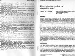
1.1.1 The Proposed 1997 UQBT Framework The UQBT framework was initially designed in 1997 by Cristina Cifuentes and Norman Ramsey. The main aim of the design was to allow for separation of machine-dependent from machine-independent concerns, by using specifications to describe machine-dependent information, and building a framework that could make use of such specifications in a machine-independent way. Figures 1.1 and 1.2 represent the architecture and data flow framework of the proposed system. This framework is described in Chapter 4, Section 4.1.

21

22

How to Read this Book Architecture Input source binary

Binary File Decoder

Target Memory Manager

Boundary Manager

Translator Core

Mapping Manager Source Target

Binary File Encoder

Output target binary

Figure 1.1: The Proposed 1997 Architecture for UQBT

Translator Core Source binary instruction stream SLED,NJMC (UVa) λ-RTL (UVa)

Source SLED constructors SSL,SRD (UQ)

Source RTLs

promotion of local variables byte swap analysis (UQ)

machine-dependent call sequence analysis machine-independent analysis control flow graph recovery (UQ)

RTLs + CFGs atomize (UQ)

Atomized RTLs + CFGs vpoback (UQ)

Inefficient target RTLs VPO (UVa) VPO

Efficient target RTLs

Assembly language RAE (UQ)

CSDL (UVa)

Target SLED constructors SLED (UVa)

Target binary instruction stream

Figure 1.2: The Proposed 1997 UQBT Framework

1.1 The UQBT Frameworks

23

1.1.2 The 1999 UQBT Framework The 1999 UQBT framework represents the original resourceable and retargetable implementation of the UQBT system that worked for several source and target machines. This framework was designed by Cristina and Mike Van Emmerik, with input from students. It was student’s Trent Waddington’s idea to try out using C as a suitable optimizer for our backend, we were initially using the VPO optimizer for one target machine only. By using the C compiler, we would not be limited to one machine but instead would be able to compile for any of numerous target machines (we used GNU’s gcc compiler). Figure 1.3 illustrates the 1999 UQBT framework, which is described at length in Chapter 4, Section 4.2. binary translation specific optimizations

HRTL

MS-RTL → translator

MS-RTLs

Semantic Mapper

Pentium Alpha Sparc CTL

HRTL

HRTL

→ low level C translator

Pentium Pentium SLED SLED Alpha Alpha Sparc Sparc PAL DCTL

Pentium SLED Alpha Sparc SSL

Low level C

MT Optimizer

MS Assembly Instructions

Instruction Decoder

MT Assembly Instructions

Pentium SLED Alpha Sparc SLED

rodata.s

MT Linker data.s

MS binary instruction stream

Binary-file Decoder

PE EXE Elf BFF MT binary file

MS binary file

Figure 1.3: The 1999 UQBT Framework

1.1.3 The 2001 UQBT Framework The 2001 UQBT framework concentrated on creating a retargetable backend, the current implementation reflects the experimentation done with four different backends–one that generates low-level C code (the 1999 backend), another that generates JVML code1 , another that generates VPO RTLs to interface with the VPO optimizer, and last, a backend to generate object code without performing register allocation to interface with 1 JVML

stands for the Java Virtual Machine Language, otherwise known as the Java bytecode language.

24


an optimizer of object code (such as a post optimizer). This experimentation reflects the ideas of Cristina and Brian in this area, as well as input from intern Manel Fernández. Figure 1.4 represents the existing implementation of the UQBT framework. This framework is explained in Chapter 4, Section 4.3. binary translation specific optimizations

M S -RTL HRTL translator

Control transfer API

MS specific code

M S -RTLs

HRTL C or M T -RTL Code Generator

Pentium SLED Alpha

JVML Code Generator

Sparc PAL

Code Expander

JVML

Sparc SSL

M S assembly instructions

Instruction Decoder

Low level C

Pentium SLED Alpha Sparc MD

Pentium SLED Alpha

C Compiler or M T Optimizer

JVML Assembler

M T binary instr stream

Optimizer

Sparc SLED

Pentium SLED Alpha Sparc MD

M T binary instr stream

rodata.s rodata.s

M T Linker Binary-file Decoder

Pentium SLED Alpha

Instruction Encoder

MT Assembly Instructions

Sparc SLED

M S binary instr stream

Sparc PAL

M T assembly instructions

Pentium SLED Alpha

Semantic Mapper

Pentium SLED Alpha

Binary File Format API

M binary file s

Binary-file Encoder

rwdata.s rwdata.s

M T binary file

JVM .class


M T binary file

Figure 1.4: The 2001 UQBT Framework Figure 1.5 illustrates the final aim of building a retargetable backend that was capable of supporting code generation at different levels of abstraction (machine code, assembly, RTL, C or JVML). Most of the infrastructure is in place at present for this framework, however, not all pieces have been factorized in order to have the common view represented in the diagram. Some of the ideas in this area are documented in Chapter 16, Section 16.1.

1.2 Roadmap There are numerous chapters in this book, some are not even part of the 2001 UQBT source code distribution, however, we have kept such chapters for their value in experiments run at some point in time. The documentation is also not complete, there are parts of the system that are not documented in these chapters,

1.2 Roadmap

25 binary translation specific optimizations

M S -RTL HRTL translator

Control transfer API M S -RTLs

MS specific code

Sparc PAL

Instruction Decoder

C or M T -RTL Code Generator

Sparc SSL

M S assembly instructions Pentium SLED Alpha Sparc SLED

Pentium SLED Alpha

M binary file s

Pentium SLED Alpha

JVML Code Generator

Low level C

JVML

C Compiler or M T Optimizer

Sparc MD


Optimizer

M T assembly instructions

M T Encoder

Sparc MD

Pentium SLED Alpha Sparc SLED

JVML Assembler M T binary instr stream

M T assembly instrs

M S binary instr stream

Binary-file Decoder

Sparc PAL

Pentium SLED Alpha

Pentium SLED Alpha

Semantic Mapper

Pentium SLED Alpha

Code Expander

HRTL

rodata.s

rodata.s

rwdata.s

Binary-file Encoder

M T Linker


rwdata.s

M T binary file

JVM .class

M T binary file

Figure 1.5: The Ideal Framework for those, you will have to refer to the source code. The following roadmap helps in understanding which parts of this book are general, which are part of the 2001 distribution and which are of historical interest. The first part of this book—Introduction—is a general overview of binary translation (Chapter 2), some previous work in the area (Chapter 3), and a summary of the three UQBT frameworks that were documented in the history of the project: the proposed 1997 framework, the 1999 implementation and the final 2001 implementation (Chapter 4). The Frontend part describes most of the components of the 1999 and 2001 UQBT frameworks when these components where built. The binary-file format API is described in Chapter 5, the decoding of machine instructions is described in Chapter 6, the specification of semantics of machine instructions is described in Chapter 7, and the internal UQBT intermediate representations used for RTL and HRTL levels are described in Chapter 8. The Analysis part deals with some of the analyses performed in abstracting away from machine dependent information (RTLs) into a high-level representation (HRTL). The analyses that are described are: how to eliminate condition codes (Chapter 9), how to remove delayed branches from the intermediate representation (Chapter 10), how to recover parameter, local variable and function return information at procedure call sites (Chapter 11), and how to perform low-level type analysis recovery (Chapter 12).

26


The Backends part deals with explanations of the four different backends that are implemented in the 2001 UQBT framework. These are: the original 1999 (low-level) C backend (Chapter 13), the 1999 and 2000 JVML backends (Chapter 14), the 1998 and 2001 VPO backends (Chapter 15), and the object code backend as well as the design of a retargetable backend (Chapter 16). There is also a standalone chapter on how to use the New Jersey Machine Code toolkit for encoding purposes, the chapter is a standalone experimentation with encoding of assembly code dynamically (Chapter 17). The Results part of the book presents results of 5 initial experimental translators (SPARC to SPARC, SPARC to Pentium, Pentium to SPARC, Pentium to Pentium, and SPARC to JVML); the results were collected in Sep 1999 (Chapter 18). Chapter 19 provides guidelines on how to instantiate a new translator using the UQBT framework, Chapter 20 contains notes from 1999 and 2001 on our experiences with building new frontends or backends for the UQBT framework. Last, Chapter 21 has some notes on ways to tackle debugging in the UQBT framework, as no built-in debugging support exists in the framework. The Runtime Support part is slim and outdated, it contains notes from early 1999 on an interpreter that was built in that year; that interpreter is not part of the distribution as it is obsolete (Chapter 22). The only Appendix that is left deals with how to configure the UQBT framework to instantiate a particular translator. These notes were written in 2001 after we stopped using multiple Makefiles and decided to use the configure system to generate our Makefile. There is also information on how to run the regression test suite. This book has not documented the graphical interface of the system, which was written in early 2000 using the tcl/tk system. You will find this interface in the gui directory of the 2001 UQBT distribution. The GUI allows for translations across some types of machines, and it produces its output in text and graphical forms. To run it, emit the following command: wish uqbt.tcl For most of the time, we used the UQBT system in a command-line fashion, as described in the Appendix.

Part I

Introduction

27

Chapter 2

Binary Translation Design: Cristina, Norman; Documentation: Cristina [c.1996]

Binary translation, the process of translating binary executables1 makes it possible to run code compiled for source platform Ms on destination platform Md . Unlike an interpreter or emulator, a binary translator makes it possible to approach the speed of native code on machine M d . Translated code may run more slowly than native code because low-level properties of machine Ms must often be modeled on machine Md . For example, the Digital Freeport Express translator (Dig95) simulates the byte order of SPARC, and the FX!32 translator (Tho96, HH97) simulates the calling sequence of the source x86 machine, even though neither of these is native to the target Alpha. Because code for decoding, analyzing, translating, and emitting machine instructions is highly machinedependent and is written by hand, existing binary translators are limited to one or two platforms. Our research makes it much easier to build binary translators for new platforms. It also lays a foundation for the development of new analyses that could improve the performance of translated code; for example, it might be possible to use native byte order or calling sequences in many cases. Commercial hardware and software companies (e.g. Digital, AT&T, Sun) have invested significant resources in the development of automatic binary translation, but some of the approaches have been constrained by time-to-market issues. Our research attacks problems that cannot be considered in a product setting scenario.

2.1 Is Binary Translation the Solution to all Migration Problems? There are different expectations from binary translation technology depending on who you are or work for. We briefly describe three different points of view to the expectations of binary translation technology based on whether you have invested in software or in hardware. 1 In this document, the terms binary executable, executable, and binary are used as synonyms to refer to the binary image file generated by a compiler or assembler to run on a particular computer.

29

30

Binary Translation

From the point of view of an organization which has invested large resources into the development of software, ideally, binary translation should aid in the migration of legacy2 applications from Ms to a newer platform Md , to take full advantage of Md ’s computing resources, but also to maximize the investment in software systems and minimize retraining costs on new systems. From the point of view of a hardware manufacturing organization which has invested large resources into the development of new state of the art computers, binary translation should aid in the fast/immediate migration of application programs to run on and benefit from the full performance of the new machines. Unless software is made available on the new machines, users will not be able to use the machines efficiently. Finally, from the point of view of a software developer, binary translation could provide the solution to making software available on a variety of hardware platforms at a reduced cost overhead due to a reduction in the testing cycle (for each different machine). Binary translation techniques aim to translate the object code (i.e. image) of an application (i.e. its binary code) from an old machine to an equivalent object code for a newer machine. Although it is not very difficult to translate some sequences of machine instructions from one machine to another, other considerations make the task very difficult in practice. For example, binary code often mixes data and instructions in the same address space in a way that cannot be distinguished given the same representation for data and code in Von Neumann machines. This problem is exacerbated with indirect or indexed jumps, where the target value of the jump is known at runtime, but hard to determine statically. Further, some of the older operating systems did not provide systems programmers with an ABI (application binary interface) to low-level system calls, hence allowing application writers to directly access the memory and by pass the operating system. All of these problems and more are common to binary-code manipulation tools such as disassemblers and decompilers, as the static parsing of the machine instructions in the binary file is a partially incomplete step given its equivalence to the halting problem (HM79) and hence undecidable in general. Nevertheless, for binary translation purposes, this does not mean that the problem cannot be solved at all. In fact, given that the translated binary file will need to be executed, the information that could not be decoded statically will be available dynamically, hence allowing for runtime translation or interpretation of the binary code. Problems that are specific to binary translation are due to the multi-platform nature of the translation: there is need to address the differences in source and target architectures (e.g. CISC vs RISC), the endianess of the machines (e.g. little vs big), machine-dependent issues (e.g. delay branches or register windows on SPARC), and compiler-generated idioms, as well as the differences in operating system services and GUI calls—which are the hardest to address. The work reported in the literature so far suggests that a new binary translator is hand-crafted to address each different pair of platforms due to machine dependency constraints. It is clear that an “all purpose” binary translator is very hard to develop, therefore some bounds for the research are established in the next section. 2 The IEEE standard 1219-1993 (IEE93) defines a legacy system as any system whose documentation does not conform to the Standard’s requirements. This normally is used to describe systems that were constructed before structured programming techniques were universally adopted. In the context of this document, legacy software is that built in the last 5 to 10 years for register-based machines, which needs to be ported/migrated to a new(er) platform.

2.2 Goals and Objectives

31

2.2 Goals and Objectives Binary translation requires such machine-level analyses as finding procedures and code attached to those procedures, finding targets for indirect transfers of control, identifying calling conventions and sequences, and recovering type information for procedure parameters. Other analyses may make it possible to improve translated code, e.g., by eliminating byte swapping, by promoting local variables to registers, or by translating platform Ms calling sequences to native platform Md calling sequences. We plan to simplify the implementation of such analyses by having them operate on register transfer lists (RTLs), a machine-independent representation of the effects of instructions. This simplification will reduce retargeting costs by making it easier to implement analyses for new platforms. Moreover, in some cases it will be possible to eliminate the retargeting cost entirely by making the analysis itself machine-independent. To use the analyses on real binary codes, we must be able to transform them into RTLs and back again. We plan to derive transformers from formal descriptions of the representation and semantics of machine instructions. The goals of the project are therefore:

to understand what aspects of instruction representation and semantics are needed to perform binary translation, to write those aspects as formal machine descriptions, to derive components of binary translators from those descriptions, to understand how to implement existing machine-dependent analyses on a machine-independent RTL representation, and to understand which of these analyses can be made machine-independent, and how, and to develop a framework for experimentation with binary manipulation ideas.

To keep things simple, translation is limited to user routines (i.e. applications programs), not kernel code or system calls (i.e. systems programs), or dynamically linked libraries (as these are sometimes written in assembly code and relate to systems programs). Note that this approach is not limiting, Digital has used it for their FX!32 hybrid translator for x86 Windows 32-bit binaries on Alpha (HH97). We are working within the context of a multi-platform operating system, Solaris, which runs on SPARC and x86 (the PowerPC version was not made available). Similar ideas work on other multi-platform OSs such as Linux and Windows NT. We also experimented with cross-OS translations where the two OSs were similar in nature; for example, Solaris and Linux. We can successfully translate (Solaris,SPARC) binaries onto (Linux,x86), provided the same libraries are made available in both systems.

2.3 Types of Binary Translation The first binary translators written, VEST and mx by Digital (SCK+ 93), were static in nature, that is, all analysis was performed statically and a fallback mechanism (an interpreter) was used at runtime to handle

32

Binary Translation

code that was not decoded statically. It has been suggested that a dynamic binary translator can be built based on dynamic compilation techniques (CM96). This would overcome the problems found with static translation but at the cost of execution time of the generated binary. At present, most dynamic compilers generate much slower code than static compilers; a factor of 2x is normally quoted. Recently, a hybrid approach was used by Digital to develop FX!32 (HH97, Tho96), a two-step translator which emulates the code the first time it is run, and binary translates it in the background once profile information has been gathered from the program’s execution. In the next subsections, we briefly explain the first two methods, the third method is reviewed in Chapter 3 along with other commercial translators.

2.3.1 Static binary translation The structure of a static binary translator is presented in Figure 2.1. The front end is a (source) machinedependent module that loads the source binary program, disassembles it, and translates it into an intermediate representation. The middle-end is a machine and operating system independent module that performs the core analysis for the translation, and as such performs optimizations on the code. The back end is a (target) machine-dependent module that generates a binary program for the target machine; performing the tasks of a traditional compiler code generator and object code emitter that assembles the code in the binary file format of the target platform. binary program (Ms,OSs)

Front-end intermediate code Analysis intermediate code’ Back-end

binary program (Mt,OSt) [including binary program (Ms,OSs)]

Figure 2.1: Structure of a static binary translator for source machine Ms , target machine Mt , source operating system OSs and target operating system OSt . The fallback mechanism used by static binary translators is a runtime environment that completely supports the source platform, and hence includes an interpreter for source machine instructions, and support for translation and mapping of operating system calls into the new platform. The development of a runtime environment is a significant overhead; especially the mapping of operating system calls. There is little performance data reported in the literature regarding the amount of time spent by binary translated applications in the interpreter mode. Code ported from a proprietary CISC to RISC machine at Tandem, where the operating system was binary translated to the new machine, reports an average figure of 1% of the time being

2.3 Types of Binary Translation

33

spent on interpretation (AS92). Informal talks with people who have developed such translators state that the interpretation mode is seldom used if you have sufficient coverage of the patterns generated by compilers commonly used in that platform. Existing static translators have dealt mainly with procedural code, rather than object-oriented code, which poses new limitations to static translation due to their dynamic nature of code dispatching through vtables.

2.3.2 Dynamic binary translator A dynamic binary translator performs the translation of the code while the program is being executed by the translator; that is, the input binary program is dynamically analyzed and translated into the target machine code during runtime. Dynamic translation techniques overcome some of the shortages of static translation, for example, determining the targets of indirect jumps. Dynamic translation is able to support most practical cases of self-modifying code; code normally not supported in static translations. Given that all the processing of a dynamic translator is done “on the fly”, the types of optimizations and analyzes have to be carefully considered and optimized so that the minimum amount of time is spent during runtime. The structure of a dynamic binary translator is depicted in Figure 2.23 . The binary program is fed into the front end which generates an intermediate representation for a block of code. This representation is then compiled or emulated by the translator to generate (unoptimized) machine code for the target machine. If at any time the translator determines that a new region of the program needs to be decoded, the front end is dynamically invoked to parse that region and provide the intermediate representation. When generating machine code, counters are kept on the number of times blocks of code are executed; once a threshold is reached, machine code is regenerated to produce better machine code—this process can be repeated several times, hence producing better code on a demand-driven basis. It is important to note that the translation is done in a lazy fashion; that is, code is only translated when its path is reached. In this way, fragments of the program that are not executed during runtime, are not translated either. Self-modifying code is handled by invalidating the existing intermediate representation and re-parsing the binary code with the changed bytes. Dynamic compilers can perform runtime optimizations of the code based on the execution profile of the program, hence several optimizations, such as dynamically-dispatched calls and procedure inlining, can only be possibly done on a dynamic compiler rather than using static techniques. The performance penalty of code generated by such a translator is estimated between 0.9X to 2.4X times that of code generated by a native optimizer C++ compiler (these figures are based on code generated by the SELF-93 dynamic compiler (Hol95)). An interesting point to note is that a dynamic binary translator for a multi-platform operating system does not require the development of a runtime environment to support the mapping of old operating system calls, as all translations are done “on the fly”. Using static techniques in this case will still require a runtime environment to cater for the interpretation of old machine instructions–dynamic techniques alleviate the need for this fallback mechanism, but compromise the speed of execution of the program at the expense of less analysis and code quality.

3 Figure

2.2 by the SELF team at Sun Microsystems Labs.

34

Binary Translation

binary program (Ms,OS)

Front-end intermediate code Compilation/Emulation machine code (Mt,OS) Optimizer

optimized machine code (Mt,OS)

Figure 2.2: Structure of a dynamic binary translator for a source machine Ms, a target machine Mt and a multi-platform operating system OS.

Chapter 3

Previous Work Documentation: Cristina [c.1996, 2001]

Binary translation is a relatively new field of research, were the techniques are derived from the compilation, emulation and decompilation areas. Nevertheless, the techniques are ad hoc in nature and little has been published about them (mainly driven by commercial interests of the parties involved). In this chapter we describe the related work, which we have classified into two main groups: works related to binary translation and interpreters (or emulators), and works related to binary-code manipulation tools that may aid in the process.

3.1 Binary translators and interpreters Binary translation techniques were developed from emulation techniques at research labs in the late 1980s. Projects like the HP3000 emulation on HP Precision Architecture computers (BKMM87) and MIMIC, an IBM System/370 simulator on an IBM RT (RISC) PC (May87) were the catalist for these techniques. One of the goals of the HP project was to run existing MPE V binaries on the new MPE XL operating system. For this purpose, a compatibility mode environment was provided, which was composed of two systems: a HP 3000 emulator and a HP 3000 object code translator. The emulator duplicated the behavior of the legacy hardware, and the translator provided efficient translated code which relied on the emulator when indirect transfers of control where met. Tandem developed an object code translator for TNS CISC binaries to TNS/R (RISC) in order to provide a migration path for existing vendor and user software (AS92). This approach allowed them to market their new RISC machines years earlier than if no migration path was available. Part of the rationale for the project was also the fact that no reprogramming was involved and that the techniques would provide faster code than emulation techniques. Less than 1% of the time was spent on emulation. Digital developed two translators, VEST and mx, to provide a migration path from their OpenVMS VAX and Ultrix MIPS systems to their new Alpha machine (SCK+ 92, SCK+ 93). Interestingly enough, they decided to do careful static translation once instead of on-the-fly dynamic translation at each execution time for 35

36

Previous Work

performance issues. In both their translators, the old and new environments were, by design, quite similar, plus both provided similar operating system services. Some of the goals were to take full advantage of the performance capabilities of the Alpha and avoiding the problem of not having all the tools available to port a program to a new architecture (because they are still not available on the new hardware). This was seen as an interim solution, while the user’s environment was made available on the new machine and then code could be recompiled/rebuilt. Up to 1992 all translators were made available by hardware manufacturers to provide a migration path from their legacy hardware platform (normally a CISC) to their new platform (normally a RISC). Back in 1994, AT&T Bell Laboratories provided services to migrate software in object code form from one platform to another through the FlashPort binary translator (T94). Translations of PDP 11, 680x0 and IBM 360 code was made to platforms like MIPS, RS/6000, PowerPC and SPARC. Translation time was based on the type of application, with some large applications being translated in 1 month, whereas others in 6 months; which means that manual changes were done to assure consistency of the translation, plus to provide compatibility libraries to cater for the differences in operating systems and services. The FlashPort technology was initially developed by Bell Laboratories researchers and was commercialized through the 1991-formed Echo Logic company. The first production release of the technology was provided to Apple Computers in 1993 to translate Macintosh binaries to the then forthcoming PowerPC-based Macintosh computers. In an attempt to make Alpha machines more appealing to existing Unix users, Digital released FreePort Express, a SunOS SPARC static binary translator to Digital Unix Alpha (Dig95); particularly at a time when Sun was migrating customers to their new Solaris OS and discontinuing support for SunOS. The tool was advertised as a way of migrating to the Alpha even when source code and compiler tools from the source machine were not available; then do a native port at your own leisure. Since the translated programs and libraries provided support for Xview, OpenLook, Motif and other X11-based applications, this migration path was suitable for users who did not want to be trained in the use of new tools. To improve Alpha’s usability as a desktop alternative to Intel PCs, Digital developed FX!32, an WindowsNT x86 to WindowsNT Alpha translator (Tho96, HH97). Emulation was used as it provided a quick way to provide support for changes in WindowsNT. However, binary translation on the background was also used in order to save the translations to a file and, over time, incrementally build the new Alpha binary. This hybrid translator uses profiling information in order to optimize the code the next time it is run. The TIBBIT project looks at real-time applications that are to be binary translated between processors of different speeds (CS95, Cog95). The translated software needs to retain the implicit time-dependency of the old software in order to function correctly. We summarize the features of a variety of binary translators and interpreters in Table 3.1. The column Purpose describes the general use of the tool, columns Source Platform and Target Platform describe the nature of the translation supported by the tool (i.e. multi-platform or within the one platform), column Name refers to the name of the software; if unnamed, then it refers to the people that worked on it, and column Affiliation refers to the affiliation of the authors of the software at the time of development.

3.1 Binary translators and interpreters

37

Name Bergh et al (1987)

Affiliation HP

Ref Purpose (BKMM87) Software emulation and object code translation.

Source Platform (HP3000, MPE V)

Mimic (1987) Johnson (1990) Bedichek et al (1990) Accelerator (1992) VEST, mx (1993)

IBM

(May87) Software emulator with a 1:4 code expansion factor per old machine instruction. (Joh90) Postloading optimizations.

IBM System/370

Target Platform (HP Precision Architecture, MPE XL) IBM RT PC

RISC

RISC

Motorola 88000

Motorola 88000

TNS CISC

TNS/R

Wabi (1994)

Sun AT&T

(VAX, OpenVMS), (MIPS, Ultrix) (x86, Windows 3.x) 680x0 Mac, IBM System/360, 370, 380

(Alpha, OpenVMS), (Alpha, OSF/1) (SPARC, Solaris)

Flashport (1994)

(Bed90) Efficient architecture simulation and debugging. (AS92) Static binary translation for CISC to RISC migration. Uses a fallback interpreter. (SCK+ 93)Static binary translation from Digital’s VAX and MIPS machines to the 64-bit Alpha. Uses a fallback interpreter. (Sun94b) Pretranslated Windows API to Unix API calls. Dynamic execution of programs. (T94) Binary translation across a variety of source and target platforms. Requires human intervention.

Shade (1994)

Sun

SPARC V8, V9

MAE (1994)

Apple

680x0

RISC-based Unix

Wahbe et al (1994) Chia (1995)

CMU

(CK94) Efficient instruction-set simulation and trace generation capability. Dynamic compilation of code. (Cor94) Macintosh environment in an XWindow, Unix RISC-based workstation. (WLG94) Adaptable binaries. Binary transformations.

PowerMac, IBM RS/6000, SPARC, HP, MIPS, Pentium SPARC V9, V8

(MIPS, Ultrix4.2)

(MIPS, Ultrix4.2)

(SPARC, Solaris)

(SPARC, Solaris)

TIBBIT (1995) Then (1995)

CMU, UO

Motorola 68000

(IBM RS/6000, AIX 3.2) (SPARC, Solaris)

Freeport Express (1995)

Digital

FX!32 (1996)

Digital

(Chi95) Software emulation within the same platform, with a 1:100 code expansion factor per old machine instruction. (CS95, Binary translation of time-sensitive applicaCog95) tions. (The95) Optimization of code within the same platform. (Dig95) Static binary translation and fallback interpreter. Translates user mode programs. 32bit to 64-bit translation. (Tho96, Hybrid emulator/binary translator of popular HH97) x86 32-bit applications to Alpha.

Stardent U.Wash Tandem Digital

Purdue

Purdue

(SPARC, Solaris) (SPARC, SunOS4.1.x)

(Alpha, OSF/1)

(x86, dowsNT)

(Alpha, dowsNT)

Win-

Win-

Table 3.1: Summary of Binary Translators and Interpreters in Cronological Order.

3.1.1 List of recent translators There has been a lot of work in the last few years (1998-2000) on dynamic techniques for doing binary manipulation of one sort of another. The following is a list of projects and literature available:

HP Aries (ZT00): Aries is a hybrid interpreter/dynamic translator which allows PA/RISC HP-UX binaries to run in an IA-64 HP-UX environment transparently, without user intervention. HP Labs Dynamo (BDB00): Dynamo is a dynamic reoptimizer of PA-RISC binaries which produces PA-RISC code. It works well for some programs and not for others.

38

Previous Work

IBM TJ Watson Research Center’s DAISY (EA96) and BOA (GAS+ 00): The DAISY and BOA projects have looked at dynamic binary translation from conventional architectures such as the PowerPC to VLIW or other novel architectures. Their work addresses precise exceptions, self-modifying code, and reordering of memory references; all of these from an architectural point of view. Transmeta’s Crusoe (GP00): The Crusoe chip is a VLIW chip which includes code morphing to dynamically binary translate from x86 to the VLIW instruction set. Some x86 instructions are supported by the hardware itself. Compaq’s Wiggins/Redstone (RDGY00): Wiggins/Redstone was a dynamic reoptimizer of Alpha binary code. It was built based on Digital’s DCPI infrastructure.

3.2 Binary-code manipulation tools Name Silberman et al (1993) QPT (1994) Shade (1994) ATOM (1994) NJMC (1994)

EEL (1995)

Ref Purpose (SE93) Framework for supporting heterogeneous instruction set architectures. (LB94) Rewrite executable files to measure program behavior. (CK94) Execution profiling of application binaries. (Dig94, Sytem for building customized program analysis tools. ES95) (RF95, Machine-independent encoding and decoding of machine inRF94a, structions via the SLED language. RF97a) (LS95) Library for editing binaries.

Platform CISC, RISC, VLIW MIPS, SPARC SPARC V8, V9 (DecStation, Ultrix), (Alpha, OSF/1) MIPS, SPARC, x86, PowerPC, Alpha MIPS, SPARC

Table 3.2: Summary of Binary-code Manipulation Tools in Cronological Order. Table 3.2 summarizes the available tools for handling machine binary code. The column Name lists the name of the tool (or its author if no name was given to the tool), column Ref lists the references in the literature to this tool, column Purpose describes the purpose of the tool, and column Platform lists the platform(s) supported by these tools. ATOM is a tool-building system that provides a flexible and efficient interface for the instrumentation of code and has been used for the construction of an instruction profiler, cache simulator and compiler auditing tool (ES95). The user needs to write an instrumentation file in terms of ATOM’s abstractions (procedures and basic blocks), and an analysis file (using a high-level language such as C) with the routines that are to be included for instrumentation purposes. The performance of the generated tools compare favourably with hand-crafted implementations of same the tools. Shade is an instruction-set simulator which optionally allows users to profile code that traces the execution of an application at runtime. Trace information on instruction addresses, instruction text, decoded opcode values, and more can be collected by Shade (CK94). This tool works only on SPARC machines. Both NJMC (New Jersey Machine-Code) toolkit (RF95, RF97a) and EEL (Executable Editing Library) (LS95) provide support for manipulating machine instructions. The NJMC toolkit supports the encoding and decoding of machine instructions for a variety of RISC and CISC machines, by means of SLED

3.2 Binary-code manipulation tools

39

specifications. The SLED language allows for the description of the syntax of machine instructions in a specification that resembles instruction descriptions found in architecture manuals. The toolkit has successfully been used in a retargetable linker (Fer95) and a retargetable debugger (RH92). The EEL library was built based on the NJMC machine specifications, and introduced control flow support based on techniques developed in the QPT (LB94) profiler. EEL also introduced limited support for describing the semantics of machine instructions. The tool is not fully portable to non RISC environments.

40

Previous Work

Chapter 4

The UQBT Framework Design: Cristina, Norman; Documentation: Cristina [c.98, May 00, Nov 01]

The University of Queensland Binary Translator (UQBT) framework, is designed to support experimentation in static binary translation. UQBT strives to adapt easily to changes in both source and target machines at low cost, including translations to register-based and stack-based machines. Support for multiple architectures is provided by means of specification of properties of machines, as well as conventions used by operating systems. This chapter describes the overall architectural organization of UQBT (Section 4.1) and its components from the point of view of instruction translation (Section 4.2). Note that these two sections are necessarily overlapping; the former section reflects more of the design and the latter section reflects more of the implementation of the system. The chapter concludes with a small section on the state of the UQBT framework at the end of 2001.

4.1 The Proposed 1997 Architecture of a Retargetable Binary Translator Like a compiler and a decompiler, a binary translator can logically be divided into three phases: front end, analysis and transformation, and back end. For a given source machine Ms and destination machine Md , the front end decodes machine Ms ’s binary file and stores the information in a machine-independent intermediate form based on RTLs. The analysis phase maps machine Ms ’s locations onto machine Md ’s locations and transforms the RTLs so that they can be readily translated into native code for machine Md . The back end translates the intermediate form and writes a binary file for machine Md . It may also optimize instructions. From a retargetability point of view, it is more helpful to think of a functional division into components instead of a sequential division into phases. Such components may be used in more than one phase. Some components will be machine-independent; others may be generated from machine descriptions. In Figure 4.1, we identify components by putting them in boxes.

41

42

The UQBT Framework

Architecture Input source binary

Binary File Decoder

Target Memory Manager

Translator Core

Boundary Manager Mapping Manager Source Target

Binary File Encoder

Output target binary

Figure 4.1: Architecture for a Retargetable Binary Translator. Components are Represented in Boxes.

Implementation of components draws on techniques developed for dcc, an 80286 decompiler (CG95), for specifying representations of machine instructions (RF97a), and for the U.S. National Compiler Infrastructure project.

4.1.1 Components Ms binary file reader exports an abstraction representing the contents of the executable binary on the original machine. This module promotes retargetability by hiding information about the source machine that one might otherwise be tempted to exploit. The capabilities exported include: 1. The initial state of the Ms processor that would apply when about to run this binary on a native Ms processor, including at minimum the value of the program counter, 2. A list of potential entry points for procedures, possibly empty (N.B. the initial program counter is always available as an entry point), 3. The ability to fetch the program’s code and data, by the address those contents would occupy in a running Ms executable, and

4.1 The Proposed 1997 Architecture of a Retargetable Binary Translator

43

4. The ability to identify calls to dynamically linked procedures, and to provide access to the code and data associated with those procedures. This module may therefore include much of the functionality of a dynamic linker/loader. One of the crucial decisions made by a translator is which locations on machine Md hold what data from machine Ms . We will encapsulate these decisions in a mapping manager, which will map locations in code space, locations in data space, and locations referring to registers or other processor state. Most mappings will be determined automatically at translation time, but some mappings may be specified by hand for each pair of platforms, e.g., what registers of machine Md should be used to represent the contents of registers of machine Ms . The mapping manager will rely on the Md memory manager to allocate locations in the destination machine’s storage space, e.g., to store translated code. Because it is impossible to identify and translate all code, a running image on machine Md will in general have a mix of translated and untranslated code. The boundary manager will track the boundary between translated and untranslated code and handle flow of control across the boundary. For example, a branch from translated to untranslated code might go to an interpreter or to a dynamic translator. If the untranslated code is subsequently translated, the boundary moves, and the boundary manager might backpatch the branch. The core translator will translate groups of machine instructions. A group may be as small as a basic block or as large as an entire program, and different translation strategies (e.g., full static, partial static, dynamic) may use different group sizes. The core translator coordinates the action of all the other components and performs the main translation analyses. It will translate a group of Ms instructions as follows: 1. Ask the memory manager for a location in Md to hold the translated code, and inform the mapping manager of the new mapping, 2. Translate Ms instructions to Md instructions

using information from the mapping manager to translate access to machine Ms ’s data, using information from the boundary manager to translate flow

of control outside the current group, and 3. Inform the boundary manager of the translation of the current group. The boundary manager may choose to backpatch branches into the current group. Depending on the granularity and timing of translation, these steps may be repeated on other units until some termination condition is met. If the granularity of translation is sufficiently large, the second step may involve translating into an intermediate form and doing some global analysis and optimization. Finally, the Md binary file writer will export an abstraction representing the ability to create an executable binary on machine Md . It will export the abilities to: 1. Specify the contents of the Md address space at the start of execution, 2. Establish the state of the Md processor at the start of execution,

44

The UQBT Framework 3. Write an executable binary file in the Md native format, and 4. Possible support for dynamic linking, e.g. of translated or native libraries.

In a dynamic translator, this component would simply write into a running process image (and possible flush the I-cache).

4.1.2 Core Translation based on RTLs The translation itself will be performed using register transfer lists (RTLs). An RTL is a collection of simultaneous effects. Each effect has the form ‘location := expression’, and the expression is always evaluated without side effects, so all state change is explicit. RTL expressions are represented as trees, the leaves of which refer to constants or to the values contained in locations. Note that although the tree leaves refer to locations, the values themselves are not necessarily calculated, only the location is referenced. The internal nodes of the trees are ‘RTL operators’. For illustrative purposes, the following is an ASCII representation of an RTL representing the effect of the SPARC andcc instruction: $r[rd] icc.N icc.Z icc.V icc.C

uNativeAddr); // Address // Compute offset from start of text section to this function dword offset = v.uSymAddr - pText->uNativeAddr; dword p = pText->uHostAddr + offset; // Start of function for (int i=0; i < n; i++) printf("%02X", *((unsigned char*)p++)); printf("\n"); } } else printf("No function ’_exit’\n"); return 0; } To compile it, at the command line type: gcc -g -o dumpexit dumpexit.cc BinaryFile.cc ElfBinaryFile.cc SymTab.cc ElfDetails.cc -lelf -lstdc++ Sample output: % dumpexit /usr/lib/libc.so.1 Function _exit (8 bytes): 000169A0: 8210200191D02008 %

5.7.3 Example 3 The following example loads the archive ”/usr/lib/libm.a” and displays the load address for the ”sin” function.

5.7 Example Code

69

#include #include "ElfArchiveFile.h" void main() { ElfArchiveFile af; if (!af.Load("/usr/lib/libm.a")) { printf("ArchiveFile could not load file\n"); return 1; } printf("There are %d members in this archive\n", af.GetNumMembers()); printf("First 5 file names:\n"); for (int i=0; i < 5; i++) { printf("%s\n", af.GetMemberFileName(i)); } BinaryFile* pm; printf("Object for function ’sin’ is at %p\n", pm = af.GetMemberByProcName("sin")); printf("Address of sin is %p; size %d\n", pm>GetAddressByName("sin"), pm->GetSizeByName("sin")); pm->UnLoad(); af.UnLoad(); } To compile, (assuming the example code is called example3.cc): gcc -g -DUNIX -o example3 example3.cc BinaryFile.cc ElfBinaryFile.cc SymTab.cc ElfDetails.cc ArchiveFile.cc ElfArchiveFile.cc -lelf lstdc++

5.7.4 Compiling and Linking Applications using the BinaryFile class need to compile the files BinaryFile.cc and ExeBinaryFile.cc (or ElfBinaryFile.cc, PEBinaryFile.cc, etc). They should link the resultant object files with the application. The final executable must be linked with the standard template library, e.g. ”lstdc++” for the GCC compiler. Elf versions also require the elf library, i.e. ”-lelf” for GCC. In addition, BinaryFile classes implementing symbol tables (at present, this is only the ElfBinaryFile class) also need to compile SymTab.cc which depends on SymTab.h, and should link with SymTab.o.

70

The BinaryFile and ArchiveFile classes

For the ElfBinaryFile class, unless NODETAILS is defined in the make (with -DNODETAILS), the file ElfDetails.cc must also be compiled and the resultant ElfDetails.o linked. In those application source files using the BinaryFile class, the appropriate header file (but not BinaryFile.h itself) should be included. For example, if using ElfBinaryFile: #include "ElfBinaryFile.h" // Definitions for the ElfBinaryFile class An example makefile fragment: OBJS = myfile1.o ... BinaryFile.o ElfBinaryFile.o SymTab.o ElfDetails.o ElfBinaryFile.o: BinaryFile.o ElfBinaryFile.h ElfDetails.h SymTab.o: SymTab.cc SymTab.h BinaryFile.o: BinaryFile.h

Chapter 6

Decoding of Machine Instructions – Syntax Parsing Design: Cristina; Documentation: Cristina [Feb 00]; Implementation: Cristina, Mike

The New Jersey Machine Code (NJMC) toolkit allows users to write machine descriptions of assembly instructions and their associated binary representations using the Specification Language for Encoding and Decoding (SLED). SLED provides for compact specifications of RISC and CISC machines; with 127, 193 and 460 lines of specification for the MIPS, SPARC and Pentium respectively. The toolkit also provides extra support for encoding of assembly to binary code, and decoding of binary to assembly code. For decoding purposes, the toolkit provides a matching statement which resembles the C switch statement. The toolkit generates C and Modula-3 code from matching statements, hence automating part of the disassembly process. The generated code can be integrated as a module of a binary-decoding application. This chapter briefly describes the SLED language, its usage for decoding of machine instructions, and the way we have optimised the the code that the toolkit generates.

6.1 SLED and Decoding of Machine Instructions This section provides a brief description of the SLED language in order to familiarize the reader with the key concepts of the language. Readers familiar with the toolkit and its usage should skip this section. A full description of the SLED language is provided in (RF97a). A complete description of the usage of the toolkit for both encoding and decoding purposes is available in the reference manual (RF94a).

6.1.1 SLED Concepts SLED introduces the following concepts to describe binary machine instructions:

71

72

Decoding of Machine Instructions – Syntax Parsing

tokens represent names for a sequence of bits. Tokens are commonly used to represent the bits of one machine instruction or of immediate operands. A token is given a size, representing the number of bits in the token. fields describe the parts of a token in terms of their name and bit range. Fields can use little or big endian conventions. patterns describe the possible values in the fields of a token, and names them. Pattern names can also refer to groups of patterns. constructors describe the mapping between binary and a symbolic assembly-like representation by associating a list of operands with a pattern. equations describe simple mathematical equations which place constraints on the values of fields used in constructors. relocatables describe operands in constructors that denote relocatable addresses. A partial example of the SPARC SLED specification is given in Figure 6.1. The fields keyword describes the specification of a token named instruction of size 32 bits. The fields of that token include: op, rd, and rs1. Each field denotes a sequence of bits of the instruction token it refers to. For example, the op field refers to bits 30 and 31, and the rs1 field refers to bits 14 to 18. By default, big-endian convention is used. The first patterns keyword defines names for 4 patterns: TABLE F2, CALL, TABLE F3, and TABLE F4. Each of these patterns bind to a value of the op field: TABLE F2 binds to 0, CALL binds to 1, TABLE F3 binds to 2, and TABLE F4 binds to 3. In this way, the 4 main tables described in the SPARC manual (spa92a) can be identified. The second patterns keyword defines names for each of the 64 values that the combination of the TABLE F3 pattern (i.e. op equal to 2) and the field op3 can take. Entries labelled denote entries without a name; i.e. entries that are not defined in the manual. The third patterns keyword defines the name arith to be any of the patterns in the right-hand side of the is keyword; namely ADD, ADDcc, TADDcc, etc. The first constructor keyword defines the constructor reg or imm to be one of two modes: immediate (imode) or register-based (rmode). The former mode binds the value of the i field to 1, and the latter to 0. The former mode returns the 13-bit value simm13 signed-extended (the ! denotes sign-extension), whereas the latter mode returns the value of the rs2 field (a register number). The second constructor keyword defines the constructor arith to require the fields and constructors rs1, reg or imm, and rd (which stand for first register operand, second register or immediate operand, and destination register). In this definition, it is implied that the bit pattern to be matched is that of the pattern arith and the fields rs1, reg or imm, and rd. In other words, this constructor defines all the arithmetic instructions for the SPARC. The last constructor keyword defines the constructor call, which takes a relocatable address (denoted by reloc). The relocatable address needs to satisfy the equation reloc = L + 4 * disp30!. That is, the relocatable address is equivalent to the sign-extended (!) 30-bit displacement (disp30) shifted left by 2 (i.e. a 32-bit address where the least two significant bits are 0) plus the current displacement (L). The value of L is obtained at runtime, by checking the address at which the CALL bit pattern is being decoded from. The call constructor is defined as the bit pattern combination of the CALL pattern and the disp30 field.

6.1 SLED and Decoding of Machine Instructions

73

fields of instruction (32) inst 0:31 op 30:31 disp30 0:29 rd 25:29 op2 22:24 imm22 0:21 a 29:29 cond 25:28 disp22 0:21 op3 19:24 rs1 14:18 i 13:13 asi 5:12 rs2 0:4 simm13 0:12 opf 5:13 fd 25:29 cd 25:29 fs1 14:18 fs2 0:4 rs1i 14:18 rdi 25:29 patterns [ TABLE_F2 CALL TABLE_F3 TABLE_F4 ] is op = {0 to patterns [ ADD ADDcc TADDcc WRxxx AND ANDcc TSUBcc WRPSR OR ORcc TADDccTV WRWIM XOR XORcc TSUBccTV WRTBR SUB SUBcc MULScc FPop1 ANDN ANDNcc SLL FPop2 ORN ORNcc SRL CPop1 XNOR XNORcc SRA CPop2 ADDX ADDXcc RDxxx JMPL _ _ RDPSR RETT UMUL UMULcc RDWIM Ticc SMUL SMULcc RDTBR FLUSH SUBX SUBXcc _ SAVE _ _ _ RESTORE UDIV UDIVcc _ _ SDIV SDIVcc _ _ ] is TABLE_F3 & op3 patterns arith is ADD | ADDcc | ADDX | ADDXcc | TADDcc | SUB | SUBcc | SUBX | SUBXcc | TSUBcc | MULScc | UMUL | SMUL | UMULcc | SMULcc UDIV | SDIV | UDIVcc | SDIVcc | SAVE |

3}

= {0 to 63 columns 4} TADDccTV | TSUBccTV | | RESTORE

constructors imode simm13! : reg_or_imm is i = 1 & simm13 rmode rs2 : reg_or_imm is i = 0 & rs2 constructors arith rs1, reg_or_imm, rd relocatable reloc constructors call reloc { reloc = L + 4 * disp30! } is L: CALL & disp30

Figure 6.1: Partial SLED specification for the SPARC

6.1.2 Decoding Using the New Jersey Machine Code Toolkit The NJMC toolkit uses matching statements to drive the decoding of a binary instruction stream. A matching statement resembles a C switch statement, except that only one arm can be matched (the first one to be valid in the instruction stream). A matching statement is identified by the match keyword. Arms of the match are identified by the | symbol, and the left and right-hand sides of the arm are separated by the => symbol. Figure 6.2 provides an EBNF-like specification of the matching statement. In that specification, pc stands

74


for the address to the instruction stream to be decoded, pattern stands for the SLED pattern to be matched (including parameters), equation stands for any valid SLED equation that needs to be valid in conjunction with a particular pattern, and code stands for the C or Modula3 code that the user wants to associate with the matched pattern. The keyword [name] is used to return the SLED base pattern name for the matched pattern. match pc to

f| pattern [fequationsg] [[name]] => code g [else code] endmatch

Figure 6.2: Matching Statement EBNF Specification For example, if the patterns add and sub are described in a SLED specification for a particular machine, then the following matching statement displays those names when matched at the binary instruction stream pointed to by the address in pc: match pc to | add (rd, rs1, rs2) => printf ("add\n"); | sub (rd, rs1, rs2) [name] => printf ("%s\n", name); | else printf ("other instruction\n"); endmatch The “arguments” to the constructor are names that match the field names defined with each constructor (in order of specification) and return the numerical value of that field. Hence, in the above example, rd, rs1 and rs2 are integers. An application writer may want to give special semantics to such returned integers; for example, displaying the name of the register instead of the integer representation of the register. If we assume we have an array of register names called reg, the above example can be re-written to also display the names of the arguments: match pc to | add (rd, rs1, rs2) => printf ("add %s, %s, %s\n", reg[rd], reg[rs1], reg[rs2]); | sub (rd, rs1, rs2) [name] => printf ("%s %s, %s, %s\n", name, reg[rd], reg[rs1], reg[rs2]); | else printf ("other instruction\n"); endmatch Matching files are processed by the toolkit to generate C or Modula-3 code that implements the decoding of the instructions in the match statement. Version 0.5 of the NJMC toolkit makes available an option to partly automate the generation of a matching statement for a particular SLED specification. The option -dis generates matching statements for the given SLED file(s) and stores them in the filename provided: -dis filename sledfile(s) In practice, the generated code needs to be modified in order to add relevant procedure names for each main matching statement, as well as remove duplicated arms from the matching statements. Note that this option is not currently available in the ML version of the toolkit.


75

Decoding of RISC Machine Instructions Some of the characteristics of RISC machines include the orthogonality of their instruction sets and the relatively small number of instructions. Further, the size of each instruction is fixed and is equivalent to the word size of the machine. These characteristics make the writing of a SLED spec and decoder easier than for a CISC instruction set. Figure 6.3 contains a snippet of code for the SPARC decoder; this code was written by hand rather than generated automatically. The main decoding routine is decode instr, which decodes one instruction per invocation. The pc argument points to the address in memory where the instruction stream to be decoded is located at. The uNativeAddr argument contains the native address where the Elf Loader would be expected to load the instruction stream, and the buf argument is a buffer where the textual assembly representation of this instruction will be stored. The code in this procedure is straight forward, except for the target address of branches and calls. Other than the type name ADDRESS, all names in uppercase represent macros used as a shorthand for invoking functions or accessing arrays of strings. Constructors for branches and calls are defined in the SLED spec as using relocatable addresses. Therefore, the toolkit generates code to return the relocated target address rather than the original offset displayed in the instruction. However, due to the fact that the toolkit is using the pc address as the address to relocate from, rather than the uNativeAddr which it does not know about, the returned target address is wrong; hence the use of a simple equation to transform the target address to the right one. The functions dis addr and dis roi implement the matching of an effective address, and a register or immediate operand, respectively. In the former function, an effective address is defined as being one of 4 cases, namely, indirect, indexed, absolute, or displacement. In the latter function, a register or immediate is either of those two options, which can also be matched against the SLED spec. Both functions return a buffer with the assembly version of the bits matched. The toolkit provides support for generating the names of registers based on the names used for patterns in the SLED spec. In a SLED spec, any name values given for fields with the fieldinfo keyword can be retrieved automatically by the toolkit in an array of strings. The command line option -lc-pat-names generates a header and data declaration file (.h and .c) with the names of all strings found in a SLED spec. In our previous example, the names for rs1 names and rd names were generated by the toolkit in a separate file and imported into the decoder (aka matcher) file. In order for the toolkit to fetch instructions from the bit stream addressed by pc in the previous example, a fetch routine needs to be provided by the tool writer. In the case of SPARC, all fetches will be 32 bits as all instructions are 32 bits, hence a fetch word function needs to be made available. Suitable code for such a function is: static ADDRESS fetch_word(ADDRESS lc) { return *(ADDRESS *)lc; } where ADDRESS is a 32-bit type. Information about the name of this function, the type of the address field, and address conversions need to be specified in an auxiliary spec. For the SPARC decoder, the interface to the instruction stream is as follows:

76 #define #define #define #define

Decoding of Machine Instructions – Syntax Parsing RD RS1 ROI ADDR

(rd_names[rd]) (rs1_names[rs1]) (dis_roi(roi)) (dis_addr(addr))

char *dis_addr(ADDRESS lc) { static char buf[512]; match lc to | indirectA(rs1) => return RS1; | indexA(rs1, rs2) => sprintf(buf, "%s+%s", RS1, RS2); | absoluteA(i) => sprintf(buf, "%d", i); | dispA(rs1, i) => sprintf(buf, "%s%s%d", RS1, (int)i < 0 ? "" : "+", i); endmatch return buf; } char *dis_roi(ADDRESS lc) { static char buf[512]; match lc to | imode(i) => sprintf(buf, "%d", i); return buf; | rmode(rs2) => return RS2; endmatch } void decode_instr (ADDRESS pc, ADDRESS uNativeAddr, char *buf) { match pc to | NOP => sprintf(buf, "nop"); | decode_sethi(imm22, rd) => sprintf(buf, "sethi %%hi(%s), 0x%x", imm22, RD); ... | alu (rs1, roi, rd) [name] => sprintf(buf, "%s %s, %s, %s", name, RS1, ROI, RD); | branchâ (tgt, a) [name] => sprintf(buf, "%s 0x%08x (%d) ; a = %d", name, tgt-pc+uNativeAddr, tgt-pc, a); | call (tgt) => sprintf(buf, "call 0x%08x", tgt-pc+uNativeAddr); | JMPL (addr, rd) [name] => sprintf(buf, "jmpl %s, %s", ADDR, RD); ... | inst = n => sprintf(buf, ".word 0x%08x", n); endmatch

Figure 6.3: Snippet Code for a SPARC Decoder

address type is "unsigned" address to integer using "%a" address add using "%a+%o"


77

fetch 32 using "fetch_word(%a)" Norman believes that in order to get the right relocated address out of branches and calls, that the address to integer option needs to be changed to something like this: address to integer using "%a - uNativeAddr + pc" In practice, this has not worked yet, and I have not tried it lately. Decoding of CISC Machine Instructions Amongst the characteristics of CISC machines are the lack of orthogonality in their instruction sets, the large numbers of machine instructions, and the variable length size for instructions. Further, assembly names are often overloaded. These characteristics make the writing of SLED specs for CISC machines harder; nevertheless, the language is expressive enough. Figure 6.4 contains part of the SLED code for the x86 instruction set. The complexity of the instruction set can be seen in terms of the number of different field definitions, the complex names used to distinguish overloaded instruction names, and the variety of values available on the right hand side of constructors. Further, the addressing modes (Eaddr and Mem) account for 10 possible combinations. The partial decoder in Figure 6.5 illustrates matching statements used to decode the x86 instruction set. The code was mostly generated automatically by the toolkit, with manual editing performed in order to remove redundant arms from the matching statements, separation of nesting of matching statements, and creation of function prototypes. The matching statement for decode instr makes use of the optional [deltaPC] notation, the effect of which is to store the number of bytes that were parsed in the deltaPC variable. This is needed by a decoder of CISC instructions as the instruction length is variable and a multiple of 1 byte. In the code provided, the address of the host instruction stream and that of the native address are given in 32-bit quantities, which means that 4 bytes can potentially be fetch, although any one particular instruction may only be 1 or 2 bytes. We use the returned deltaPC value to update the host pointer by the necessary amount. Characteristics of the generated code include the abstraction of the assembly print and file descriptor used—asmprint and asmprintfd respectively. These can be defined in any suitable way in the tool writer’s code; in our case, we defined them as fprintf and stdout respectively. The toolkit also generates functions to print signed and unsigned integer values, dependeing on their size; for example, print signed i8 to print an 8-bit signed integer. Functions to print registers may depend on the context of the instruction; i.e. the register number may be that of a byte, 2-byte or 4-byte register, which equates to different ascii representation of registers (e.g. AL or AX or EAX). In this case, the toolkit generates code to print the decimal value of the register (i.e. 1, 2 or 4). I modified this function manually to display 32-bit registers for disassembly purposes – this code is not correct for all cases and can be corrected by passing an extra argument to the print function with the size of the register operand. For CISC machines, the toolkit will need to fetch bits in different byte granularities. For x86, 1, 2 or 4 bytes may need to be fetched at any point in time. This information, along with address information, is stored in the instruction stream interface file, as follows: fetch 8 using "getByte(%a)" fetch 16 using "get2Bytes(%a)" fetch 32 using "get4Bytes(%a)"

78


fields of opcodet (8) row 4:7 col 0:2 page 3:3 sr4 3:5 sr16 0:2 r16 0:2 r8 0:2 fields of modrm (8) mod 6:7 reg_opcode 3:5 r_m 0:2 fields of I8 (8) i8 0:7 patterns arith is any of [ ADD OR ADC SBB AND SUB XOR CMP ], which is row = {0 to 3} & page = [0 1] [ Eb.Gb Ew.Gw Gb.Eb Gw.Ew AL.Ib AX.Iw ] is col = {0 to 5} patterns arithI

is any of [ ADDi ORi ADCi SBBi ANDi SUBi XORi CMPi ], which is (Eb.Ib | Ew.Iw | Ew.Ib); reg_opcode = {0 to 7} ...

relocatable d a constructors Indir [reg] : Mem { reg != Disp8 d[reg] : Mem { reg != Disp32 d[reg] : Mem { reg != Abs32 a : Eaddr Reg reg : Eaddr Index [base][index * ss] : mod = 0 Index8 d[base][index * ss] : mod = 1 Index32 d[base][index * ss] : mod = 2 ShortIndex d[index * ss] : mod = 0 E Mem : Eaddr is Mem constructors arithˆ"iAL" arithˆ"iAX" arithˆ"mrb" arithˆ"mrw" arithˆ"rmb" arithˆ"rmw" arithIˆ"wb" arithIˆ"b" arithIˆ"w"

i8 i16 Eaddr, reg8! Eaddr, reg! reg8!, Eaddr reg!, Eaddr Eaddr, i8! Eaddr, i8 Eaddr, i16

is is is is is is is is is

4, reg != 5 } is mod = 0 & r_m = reg 4 } is mod = 1 & r_m = reg; 4 } is mod = 2 & r_m = reg; is mod = 0 & r_m = 5; is mod = 3 & r_m = reg Mem { index != 4, base != 5 } is & r_m = 4; index & base & ss Mem { index != 4 } is & r_m = 4; index & base & ss; i8 Mem { index != 4 } is & r_m = 4; index & base & ss; i32 Mem { index != 4 } is & r_m = 4; index & base = 5 & ss; i32

arith & arith & arith & arith & arith & arith & (Ew.Ib; (Eb.Ib; (Ew.Iw;

= d = d = d

AL.Ib ; i8 AX.Iw; i16 Eb.Gb; Eaddr & reg_opcode Ew.Gw; Eaddr & reg_opcode Gb.Eb; Eaddr & reg_opcode Gw.Ew; Eaddr & reg_opcode Eaddr) & arithI; i8 Eaddr) & arithI; i8 Eaddr) & arithI; i16

Figure 6.4: Partial SLED Spec for the x86 Instruction Set

address type is "unsigned" address add using "(unsigned)%a + %o"

i8 = d i32 = d i32 = a

= = = =

reg8 ... reg ... reg8 ... reg ...

6.2 Recovery of Jump Table Case Statements from Binary Code

79

address to integer using "%a" And the user is required to provide the implementation for the functions getByte, get2Bytes and get4Bytes.

6.1.3 Cost of Decoding Machine Instructions Some experimentation in this area was done in 1998 in order to determine bottlenecks in the generated code and store it in a different way. The work was never finished and neither Norman nor Cristina had the time to make changes. The current NJMC implementation for generating C code from matching files is to use a decision tree for all options available in a match statement. In these decision trees, every option is inline expanded. The tree is then turned into a DAG and only at leaf nodes are goto statements used. In the generated code, switch statements are used for the different options in the decision tree. The main problem for performance of the current generated code seems to be that the code is too large to fit into the icache. This implies that there is too much inlining being done in the code. Possible optimizations that can be done to reduce this penalty are:

recognize common subexpressions and create procedures for them, convert some of the switch statements into table-driven lookup statements, and choose an appropriate numbering scheme to eliminate the table lookup (e.g. x x or x x 20 j 17) in order to cheaply compute the equivalent table lookup.

In the case of SPARC, the table-driven implementation may look like a small decision tree (with 4 branches for the main 4 cases, and one of them with extra branches), and decision tables for the n decision trees removed.

6.2 Recovery of Jump Table Case Statements from Binary Code One of the fundamental problems with the analysis of binary (executable) code is that of recognizing, in a machine-independent way, the target addresses of n-conditional branches implemented via a jump table. Without these addresses, the decoding of the machine instructions for a given procedure is incomplete, leading to imprecise analysis of the code. The standard method of decoding machine code involves following all reachable paths from the entry point (SCK+ 93, CG95). This method does not give a complete coverage of the text space in the presence of indirect transfers of control such as indexed jumps and indirect calls. A common technique used to overcome this problem is the use of patterns. A pattern is generated for a particular compiler to cater for the way in which the compiler, or family of compilers, generate code for an indexed jump. This technique is extensively used as most tools deal with a particular set of compilers; for example, TracePoint only processes Windows binaries generated by the Microsoft C++ compiler (Tra97). In the presence of optimized code, patterns do not tend to work very effectively, even when the code is generated by a compiler known to the pattern recognizer.

80


In this section we discuss our technique for recovering jump tables and their target addresses in a machine and compiler independent way. The technique is based on slicing and copy propagation. The assembly code of a procedure that contains an indexed jump is transformed into a normal form which allows us to determine where the jump table is located and what information it contains (e.g. offsets from the table or absolute addresses). The presented technique has been implemented and tested on SPARC and Pentium code generated by C, C++, Fortran and Pascal compilers. Our tests show that up to 90% more of the code in a text segment can be found by using this technique, when compared against the standard method of decoding. The technique was developed as part of our resourceable and retargetable binary translation framework UQBT; however, it is also suitable for other binary-manipulation and analysis tools such as binary profilers, instrumentors and decompilers.

6.2.1 Compiler Code Generation for N-Conditional Branches N-conditional branches were first suggested by Wirth and Hoare in 1966 (WH66, Wra74) as a useful extension to the Algol language. An n-conditional branch allows a programming language to determine one of n branches in the code. This extension was implemented in Algol 68 in a form that allowed its use as a statement or an expression. In other words, the result of the case statement could be assigned to a variable. This high-level statement has evolved to the well known switch statement in C and the case statement in Pascal, where labels are used for the different arms of the conditional branch, and a default arm is allowed, as per Figure 6.6. The C code shows the indexed variable num which is tested against the values in the range 2 to 7 for individual actions, and if not successful, defaults to the last default action. Although not commonly documented in compiler textbooks, compiler writers generate different types of machine code for n-conditional branches. These ways of generating n-conditional branches are determined by talking to compiler writers or reverse engineering executable code. Several techniques for generating nconditional branches from a compiler were documented in the 1970s and 1980s, when optimization for space and speed was an important issue. The most common techniques are described here based on (Sal81). The simplest way of generating code for an n-conditional branch is as a linear sequence of comparisons against each arm in the statement. This form is efficient for a small number of arms, typically 4 or less. A more sophisticated technique is the if-tree, where the selection is accomplished by a nested set of comparisons organized into a tree. The most common implementation is a jump table, which may hold labels or offsets from a particular label. This implementation requires a range test to determine the membership of values on the table. Although jump tables are the fastest method when there are many arms in the n-conditional branch, jump tables are space-wise inefficient if the case values are sparse. In such cases, a search tree is the most convenient implementation. When the arms of the n-conditional branch are sparse but yet can be clustered in ranges, a common technique used is to combine search trees and jump tables to implement each cluster of values (HM82, FH91). This section deals with the issue of recovering code from generated jump tables, in such a way that the target addresses of an indexed jump are determined. For an n-conditional branch implemented using a jump table, an indexed table is set up with addresses or offsets for each of the cases of the branch. The table itself is located in a read-only data section, or mixed in with the text section. In the interest of efficiency, range tests for such jump tables need to be concise. The most common way of doing both tests is as follows (Ber85):


81

k numu ) X jmp [T + (var - numl ) * w] where var is a local variable, for example [ebp-8], numu is the upper bound for the n-conditional branch, for example 7, numl is the lower bound of the n-conditional branch, for example 2, T is the indexed table’s address (and is of type address), for example 0x8048a0c, and w is a constant equivalent to the size of the word of the machine; 4 in this example. Based on this information, we can infer that the number of elements in the indexed table is numu - numl + 1, for a total of 6 in the example. The example also shows that the elements of the indexed table are labels (i.e. addresses) as the jump is to the target address loaded from the address at 0x8048a0c + ([ebp-8] - 2) * 4 . The previous example only shows one of several normal forms that are used to encode n-conditional branches using a jump table. We call the previous normal form type A. Figure 6.12 shows the 3 different normal forms that we have identified in executable code that runs on SPARC and Pentium. Normal form A (address) is for indexed tables that contain labels as their values. Normal form O (offset) is for indexed tables that contain


85

offsets from the start of the table T to the code of each case. Normal form H (hashing) contains labels or offsets in the indexed table. Form O can also be found in a position independent version as well. Normal form H contains pairs (,) at each entry into the jump table. In our 4 examples of Figures 6.7 to 6.10, we find the following normal forms, respectively:

jcond (r[24] > 5) 0x80489dc jmp [0x8048a0c + (r[24] * 4)]

) normal form A jcond (r[9] > 5) 0x10980 jmp [0x10908 + (r[9] * 4)]

) normal form A jcond ((r[8] - 67) > 53) 0x18804 jmp [0x1886c + (((((((r[8] - 67) >> 4) asmprintf (asmprintfd, "%s", print_unsigned_r32(reg)); endmatch } static void print_signed_reg(int reg) { static char *r32_names[] = { "EAX", "ECX", "EDX", "EBX", "ESP", "EBP", "ESI", "EDI", }; asmprintf(asmprintfd, "%s", r32_names[reg]); // asmprintf(asmprintfd, "%d", reg); } static void print_signed_i8(int /* [-128..127] */ i8) { asmprintf(asmprintfd, "%d", i8); } unsigned decode_instr (unsigned pc, unsigned uNativeAddr) { unsigned deltaPC; // # of bytes parsed by decoder match [deltaPC] pc to | ADDrmw(reg, Eaddr) => asmprintf(asmprintfd, "%s", "ADDrmw "); print_signed_reg(reg); asmprintf(asmprintfd, "%s", ", "); print_Eaddr(Eaddr); | ADDrmb(reg8, Eaddr) => asmprintf(asmprintfd, "%s", "ADDrmb "); print_signed_reg(reg8); asmprintf(asmprintfd, "%s", ", "); print_Eaddr(Eaddr); asmprintf(asmprintfd, "\n"); | ADDiw(Eaddr, i16) => asmprintf(asmprintfd, "%s", "ADDiw "); print_Eaddr(Eaddr); asmprintf(asmprintfd, "%s", ", "); print_signed_i16(i16); | ADDiAL(i8) => asmprintf(asmprintfd, "%s", "ADDiAL "); print_signed_i8(i8); asmprintf(asmprintfd, "\n"); ... endmatch return deltaPC; }

Figure 6.5: Snippet Code for an x86 Decoder


#include int main() { int num; printf("Input a number, please: "); scanf("%d", &num); switch(num) { case 2: printf("Two!\n"); break; case 3: printf("Three!\n"); break; ... case 7: printf("Seven!\n"); break; default: printf("Other!\n"); break; } return 0; }

Figure 6.6: Sample switch program written in the C language.

movl subl cmpl ja jmp

-8(%ebp),%eax $0x2,%eax $0x5,%eax 0xffffffd9 *0x8048a0c(,%eax,4)

8048a0c: 8048a10: 8048a14: 8048a18: ...

64 78 8c a0

89 89 89 89

04 04 04 04

08 08 08 08

! ! ! ! !

Read index variable Minus lower bound Check upper bound Exit; out of range Indexed, scaled jump

! ! ! !

Table of addresses to code handling the various switch cases

Figure 6.7: Pentium assembly code for sample switch program, produced by the Sun cc compiler.

89

90


ld add cmp bgu sethi or sll ld jmp nop

[%fp - 20], %o0 %o0, -2, %o1 %o1, 5 0x10980 %hi(0x10800), %o0 %o0, 0x108, %o0 %o1, 2, %o1 [%o0 + %o1], %o0 %o0

10908: 1090c: 10910: 10914: ...

0x1091c 0x10930 0x10944 0x10958

! ! ! ! ! ! ! ! !

Read index variable Minus lower bound Check upper bound Exit if out of range Set table address (continued) Multiply by 4 Fetch from table Jump

! Table of pointers

Figure 6.8: SPARC assembly code for sample switch program, produced by the Sun cc compiler.


18524: 18528: 1852c: 18530: 18534: 18538: 1853c: 18540: 18544: 18548: 1854c: 18550: 18554: 18558: 1855c: 18560: 18564: 18568: 1856c: 18570: 18574: 18578:

ld sub cmp sethi bgu nop or srl sll add and sll ld cmp be cmp be nop add and ba nop

[%fp - 20], %o0 %o0, 67, %o0 %o0, 53 %hi(0x18800), %o2 0x18804

! ! ! ! !

Read indexed variable Subtract lower bound Compare with range-1 Set upper table addr Exit if out of range

%o2, 108, %o2 %o0, 4, %o1 %o1, 1, %o1 %o1, %o0, %o1 %o1, 15, %o1 %o1, 3, %o4 [%o4 + %o2], %o3 %o3, %o0 0x1885c %o3, -1 0x18804 %o4, 8, %o4 %o4, 120, %o4 0x18554

! ! ! ! ! ! ! ! ! ! ! ! ! ! !

Set lower table addr Hash... ... ...function Modulo 16 Multiply by 8 First entry in table Compare keys Branch if matched Unused entry? Yes, exit (delay slot) No, linear probe with wraparound Continue lookup

1885c: 18860: 18864: 18868:

add ld jmp nop

%o4, %o2, %o4 [%o4 + 4], %o0 %o0

! Point to first entry ! Load second entry ! Jump there

91

! Each entry is a (key value, code address) pair 1886c: 0x0 18870: 0x187b4 ! Case ’C’+0 18874: 0xffffffff ! Unused entries have -1 (i.e. 0xffffff) as ! the first entry 18878: 0x18804 1887c: 0x10 18880: 0x185b8 ! Case ’C’+0x10 = ’S’ 18884: 0x2f 18888: 0x18630 ! Case ’C’+0x2f = ’r’ ...

Figure 6.9: SPARC assembly code from the vi program, produced by the Sun cc version 2.0.1 compiler.

92


8057d90: 8057d93: 8057d95: 8057d98: 8057d9e: 8057da0: 8057da3: 8057da9: 8057dab: 8057dae: 8057db3: 8057db6: 8057db8: 8057dba: 8057dbc: 8057dbf: ... 8058045: ... 805f5e8: 805f5ec: ...

movb testb setne andl testb setne andl testb setne andl shll shll orl orl cmpl jbe

38(%eax),%al $0x2,%al %edx $0xff,%edx $0x4,%al %ecx $0xff,%ecx $0x8,%al %eax $0xff,%eax $0x2,%edx %ecx %edx,%ecx %eax,%ecx $0x7,%ecx 0x280

jmp

*0805f5e8(,%ecx,4) ! Table jump

f8 7d 05 08 01 80 05 08

! ! ! ! !

Get struct member Test bit To boolean To byte Test another bit

! Save in cl ! Test third bit ! ! ! ! ! ! !

Save in al To bit 2 To bit 1 Combine these two Combine all three Upper bound compare Branch if in range

! table of addresses of code to ! handle switch cases

Figure 6.10: Pentium assembly code from the m88ksim program, produced by the Sun cc version 4.2 compiler.

#define FPSIZE(ir)

((((ir->p->flgs.dest_64) ? 1 : 0) p->flgs.sl_64) ? 1 : 0) p->flgs.s2_64) ? 1 : 0))

switch (FPSIZE(ir)) { case SSS: /* other code */ /* other cases */ }

Figure 6.11: C source code for example in Figure 6.10

6.2 Recovery of Jump Table Case Statements from Binary Code Type A

Normal Form jcond (r[v] > numu ) X jmp [T + * w]

O

jcond (r[v] > numu ) X jmp [T + * w] + T or jmp PC + [PC + ( * w + k)] jmp PC + [PC + ( * w + k)] + k jcond (r[v] > numu ) X

H

jmp [T + (( & mask) * 2*w) + w]

Types of allowed r[v] r[v] - numl ((r[v] - numl ) > 24) r[v] r[v] - numl ((r[v] - numl ) > 24) ((r[v] - numl ) > 24) ((r[v] - numl ) >> s) + (r[v] - numl ) ((r[v] - numl ) >> 2*w) + ((r[v] - numl ) >> 2) + (r[v] - numl )

Figure 6.12: Normal forms for n-conditional code after analysis

Benchmark awk vi (2.5) vi go m88ksim gcc compress li ijpeg perl vortex total

A 0 10 0 0 0 0 0 0 0 0 0 10

O 2 1 13 5 10 153 0 3 3 32 21 243

H 0 9 0 0 0 0 0 0 0 0 0 9

Unknown 0 0 1 0 2 1 0 0 1 0 0 5

Figure 6.13: Number of indexed jumps for SPARC benchmark programs

Benchmark awk vi go m88ksim gcc compress li ijpeg perl vortex total

A 6 12 5 17 207 0 3 7 36 13 306

O 0 0 0 0 0 0 0 0 0 0 0

H 0 0 0 0 0 0 0 0 0 0 0

Unknown 0 2 0 0 5 0 0 0 1 6 14

Figure 6.14: Number of indexed jumps for Pentium benchmark programs

93

94


Program awk vi (2.5) vi go m88ksim gcc compress li ijpeg perl vortex

w/o analysis 22% 24% 30% 91% 37% 58% 91% 33% 20% 10% 70%

with analysis 64% 93% 95% 100% 69% 89% 91% 36% 22% 99% 79%

difference 42% 69% 65% 9% 32% 31% 0% 3% 2% 89% 9%

Figure 6.15: Coverage of code for SPARC benchmarks

Program awk vi go m88ksim gcc compress li ijpeg perl vortex

w/o analysis 22% 28% 89% 36% 52% 84% 24% 18% 9% 68%

with analysis 65% 88% 99% 73% 86% 84% 26% 20% 99% 75%

difference 43% 60% 10% 37% 34% 0% 2% 2% 90% 7%

Figure 6.16: Coverage of code for Pentium benchmarks


10a58: 10a5c: 10a60: 10a64: ... sethi add ... ld sub cmp bgu sll ld jmp nop

0x0009c 0x000dc 0x000fc 0x0011c

! Indexed table ! of offsets

%hi(0x10800), %l1 %l1, 0x258, %l1

! Set table address ! into %l1

[%fp - 4], %l0 %l0, 2, %o0 %o0, 5 0x10b14 %o0, 2, %o0 [%o0 + %l1], %o0 %o0 + %l1

! ! ! ! ! ! ! !

95

Read idx variable Subtract min val Cmp with range-1 Exit if out of range Multiply by 4 Fetch from table Jump to table+offset Delay slot instr

Figure 6.17: Form O example for SPARC assembly code.

ldsb clr sub cmp bgu sll 43eb8: call sethi or add ld jmp nop

[%l6], %o0 %i3 %o0, 2, %o0 %o0, 54 0x44acc %o0, 2, %o0

! ! ! ! ! !

Get switch var (Not relevant) Subtract min value Cmp with range-1 Exit if out of range Multiply by 4

.+8 %hi(0x0), %g1 %g1, 0x1c, %g1 %o0, %g1, %o0

! ! ! ! ! ! ! !

Set %o7 = pc Set %g1 = 0x0001c

[%o7 + %o0], %o0 %o7 + %o0

43ed4: 43ed8: 43edc:

0x0021c 0x00af4 0x000f8

43ee0: ...

0x008d0

%o0 = 0x43eb8 + 0x1c = 0x43ed4 Fetch from table Jump to table+offset Delay slot instr

! Table of offsets from ! call instr to case code ! e.g. 0x43eb8 + 0x00f8 ! = 0x43fb0

Figure 6.18: Form O example for SPARC assembly code (vi 2.5) using position independent code. Offsets are relative to the address of the call instruction.

96

4233c: call sethi ldsb add add sub mov mov cmp add bgu sll ld jmp nop


.+8 %hi(0xfffffc00), %o2 [%i5], %o0 %o2, 736, %o2 %o2, %o7, %o2 %o0, 2, %o0 %o1, %o7 %o2, %o1 %o0, 54 %l1, 1, %l1 0x42f58 %o0, 2, %o0 [%o0 + %o1], %o0 %o0 + %o1

! ! ! ! ! ! ! ! ! ! ! ! ! ! !

Set %o7 = pc %o2 = -1024 %o0 = %o2 = -288 %o2 = pc-288 Subtract min value (Not relevant) %o1 = Cmp with range-1 (Not relevant) Exit if out of range Multiply by 4 Fetch from table Jump to table+off Delay slot instr

(288 bytes earlier than the call instruction): 4221c: 0x298 ! Table of offsets from 42220: 0xd3c ! table to case code 42228: 0x15c ! e.g. 0x4221c + 0x15c ! = 0x42378 4222C: 0x8fc ...

Figure 6.19: A different form O example for SPARC assembly code, also using position independent code. This code is generated from the same source code as the example in Figure 6.18, but with a different version of the compiler. Offsets are relative to the start of the table.

Chapter 7

Specifying Semantics of Machine Instructions Design: Shane and Cristina [97]; Documentation: Cristina and Shane [97], Nathan [Jul 01]; Implementation: Shane [97], Doug [98], Nathan [Jun 01]

A Semantic Specification Language, SSL, has been developed in collaboration with Shane Sendall (Sen97) in order to describe the semantics of machine instructions. Shane’s approach was based on an informal refinement of Object-Z (DR97) specifications he wrote for the SPARC and 80286 architectures. The original Object-Z specifications are available in his Honours thesis (Sen97); the SSL language has been modified since then and is described in this chapter. The informal refinement from Object-Z specifications faced some problems mainly to do with the bridging of the high-level specification to a concrete form. Further, the addressing modes were not specified as such but the effective address was used (this address being returned by NJMC’s matching statement). The instructions that are the harder ones to describe are higher-order instructions, which normally refer to the next instruction in the sequence. Examples of such instructions are SPARC’s delayed branches and 80286’s string repeat instructions. These will be described in more detail in Section 7.5.1.

7.1 Design Decisions The SSL language was developed with integration into the SLED language (RF97a, RF95) in mind. However, due to time constraints, the language has been interfaced to the NJMC toolkit’s matching statement construct via a library. This interface is called the RTL interface and is described in Chapter 8, Section 8.1. The following requirements were sought out of SSL:

provide a simple and compact notation, model the semantics of machine instructions separately or per groups of instructions, 97

98


model basic transfers of information via registers and memory locations, model complex and basic instructions without introduction of recursion or function calls, strictly model sizes of operands, registers and memory accesses, provide a universal model for flags and their interactions via named registers and macro “functions”, and model broad environment structure and semantics to handle many architectures and their idiosyncrasies; in other words expressibility,

Out of these requirements, the architecture environment is not yet fully supported, but will be discussed in Section 7.4.

7.2 Register Transfer Lists Register transfer lists (RTL) is an intermediate language that describes transfers of information between register-based instructions. RTL assumes an infinite number of registers, hence it is not constrained to a particular machine representation. RTL has been used in the vpo optimiser (BD88) for storing the target assembly instructions, and was a suitable representation for optimisation purposes. More recently, RTL has been used as an intermediate representation in different system tools such as the link-time optimiser OM (SW93a, Dig94), GNU’s compilers (Sta93), and the editing library EEL (LS95). In all these tools, RTL stands for register transfer language, and the representations vary widely. The literature does not give much information on OM’s RTL, but does document the other two. GNU’s RTL is a high-level language description of instructions, in a lisp-like form. A simple arithmetic operation between x and y (with size field m) is described as follows: (plus:m x y) However, high-level instructions are also modelled in the language, such as a multiexit conditional (switch in C or case in Pascal): (cond [test1 value1 test2 value2 ...] default) These high-level instructions are hard to recover from binary code and are also at a too high-level for analysis purposes. EEL uses an RTL format internally to capture the semantics of machine instructions. EEL’s spawn language extends EEL’s RTL by adding a method to express instruction semantics by the way of a simple attribute description. Spawn’s RTL defines the syntax of machine instructions in the SLED style, and the semantics as attributes to each instruction by binding instructions to their semnatic attributes. The following example describes the syntax in pat constructs, and the semantics in sem constructs. The syntax for load, store and other instructions are listed. The semantics for load instructions is given as well.

7.3 Semantic Specification Language Description pat [

ld ldub lduh ldd st _ ldsb ldsh _ _ lda lduba lduha ldda sta _ ldsba ldsha _ _ is op3inst && op3=[0b000000..0b011111]

sem [

ldsb ldsh ldub lduh ld ldsba ldsha lduba lduha lda is (\r.\m.\sgn. r[rd]:=sgn m[addr]) @ [ R4w’ R4w’ R4w’ R4w’ R4w’ R4w’ R4w’ R4w’ R4w’ R4w’ $ [ M1r M2r M1r M2r M4r M1r M2r M1r M2r M4r $ [ # # Id32 Id32 Id32 # # Id32 Id32 Id32

99 stb ldstub stba ldstuba

sth _ stha _

ldf

lddf

std swap stda swapa

]

] F4w’

F8w’

M4r

M8r

Id32

Id64

] ] ]

It can be seen from this example that this language models the semantics of instructions in a simplistic way which only covers general semantic content. The language does not cover flag effects or machine-dependent semantic attributes such as register windows on SPARC. Given the suitability of RTL as an intermediate representation for storing the semantics of instructions, we have developed our own RTL that captures enough information of machine instructions for the purposes of binary translation. We are not interested in a general RTL that would be suitable for emulation purposes, so certain low-level details have been excluded from our representation. SSL is the language we use to specify the semantics of machine instructions in terms of RTLs. We do not give a syntax description of our RTL here, but explain what the SSL language is able to specify and provide examples. Chapter 8, Section 8.1 gives a full description of our RTL language.

7.3 Semantic Specification Language Description This section describes the syntax and semantics of the Semantic Specification Language, SSL. The syntax of SSL is defined in Extended-Backus-Naur-Form (EBNF), and semantics of SSL is described in natural language integrated with examples from the 80286 and SPARC architectures. This was written in late 1997. Currently, SSL is limited in its ability to define the environment structure, and therefore such things like register windows cannot be modelled well. SSL allows for the description of the semantics of a list of instructions by means of statements or register transfers (or effects in Norman’s documentation). Most statements are assignment statements, but there is also support for conditional and flag statements. The register transfers for a group of instructions can be grouped via a table. Individual assignment register transfers allow for a variety of expression (arithmetic, bitwise, logical and ternary). The base elements of an expression are values, and the base elements of an instruction are variables. We explain each of these in detail in the next sections.

100


7.3.1 Registers A register is a named memory space, which has a size and is mapped to a particular location or sets of locations. Some registers actually overlap with other registers, for example, on x86, the 16-bit ax register overlaps with the lower part of the 32-bit eax register. On SPARC, 64-bit floating point registers are used by functions by overlapping two 32-bit registers. We introduce the concepts of ”shares” and ”covers” to specify these two types of registers. Registers are defined within the pre-defined keyword @REGISTERS. Each register has the form name[number] which is the name of the register and its size in bits. Registers can map to indexed locations in the register address space in different ways:

Numeric index: a numeric index basically gives the index into the register space. For example, %l0[32]->16 states that register name %l0 maps to position 16. Covers index: a COVERS index gives a numeric index into the register address space and also states that the register being defined covers the address space of two or more registers (i.e. from the index of the first register to the index of the last register mentioned). These registers need to be contiguous. For example, %f0to1[64]-> 64 COVERS %f0..%f1 gives register %f0to1 the indexed location 64 and states that this register overlaps the addressing space of registers %f0 and %f1. Shares index: a SHARES index gives a numeric index into the register address space and also states that the register being defined shares part of larger register (i.e. some bits are shared). For example, %ax[16] -> 0 SHARES %eax@[0..15] gives register %ax the index value of 0 and states that %ax is a 16-bit register composed of the bits 0 to 15 of register %eax. -1 index: special registers such as PC are not given positive indexed into the register address space, instead, they are listed as -1.

registers: | | |

numberRegister coversRegister sharesRegister minusOneRegister

7.3.2 Variables and Values A variable can be a register, memory, or parameter to an instruction operand. A value is the contents of a variable (denoted with the prefix prime symbol (’)) or a numerical constant (integer or float). A value can be signed extended by means of the ! symbol. For example, r[5] is register 5, and ’m[100000]! is a sign-extended value of the memory location 100000. var_op: | |

REG_ID REG_MEM_IDX_ID PARM

value_op:

’\’’ var_op

exp

’]’

7.3 Semantic Specification Language Description | | | | | REG_ID:

’\’’ ’(’ var_op oper value_op ’)’ NAME FLOAT NUM PARM "%"[A-Za-z][A-Za-z0-9]*

REG_MEM_IDX_ID: |

"r[" "m["

ADDR:

"a["

PARM:

[a-z][a-z0-9_]*

NAME:

[A-Z][A-Z0-9_]*[A-Z0-9]

FLOAT:

(-)[0-9]+.[0-9]+

NUM: | |

101

// Floats must have decimal pt

(-)[0-9]+ Ox[A-F0-9]+ (-)"2**"[0-9]+

7.3.3 Constants Constants are names assigned to numerical values that do not change. Constants are commonly used to describe fixed values of a machine, for example, WORD := 32. constants:

NAME ":=" NUM

or *80* %st := log2(2.7182818);

7.3.4 Functions Several functions are provided to allow complex instructions to be described. The main groups are conversion functions, floating point stack pseudo-functions, and transcendental functions. The conversion functions all take an expression and two integer sizes, and are used to change the size of floating point numbers, or to change from an integer of one size to a floating point value of another size, etc: fsize(exp, size1, itof (exp, size1, ftoi (exp, size1, fround(exp,size1,

size2) size2) size2) size2)

// // // //

Convert Convert Convert Convert

from from from from

float size1 to float size2 integer size1 to float size2 float size1 to integer size2 float size1 to float size2,

102

Specifying Semantics of Machine Instructions // but integer value with rounding, // e.g. 3.75 -> 4.00

To represent the effect of pushing or popping from a stack of registers, there are two pseudo-functions: FPUSH FPOP

// Signify a push to a stack of registers // Signify a pop from a stack of registers

These are used for example when describing Intel floating point instructions such as FLD. When the Register Transfer Lists are converted to independent form, these pseudo-functions must be removed with a special pass. (This pass also adjusts various register numbers, so that an equivalent representation using a ”flat” set of registers is obtained). Except just after decoding instructions, FPUSH and FPOP will not be seen. Various transcendental functions are included to describe complex floating point instructions: sin(exp) cos(exp) tan(exp) arctan(exp) log2(exp) loge(exp) log10(exp) sqrt(exp)

// // // // // // // //

Sinusoid Cosine Tangent Inverse tangent Logarithm to base 2 Natural logarithm Logarithm to base 10 Square root

All these functions take and return a floating point value.

7.3.5 Expressions Three groups of expressions are supported: unary, binary and ternary, each with an expressions as a member. Expressions are thought of as trees, with the leaves being the values of the expression and the inner nodes being the operators of the expressions. Unary expressions include the negation (NOT) of an expression, and the sign extension (!) of an expression. Binary expressions include arithmetic, floating point arithmetic, bitwise and logical expressions, as well as bitwise expressions (@). The first three types of expressions are commonly found in most languages. The latter expression, bitwise-extraction, is needed to extract bits of a field, and hence the top and bottom bits need to be specified (separated by a : and stored as a binary expression). This expression is derived from the SLED language. Examples of each of these types of expressions follow: ’r[1] + ’r[5] ’r[31] +f ’r[32] ’r[1] | ’m[1000] ’r[5] or ’r[1] ’r[5] @ [0:19]

// // // // //

arithmetic floating point arithmetic bitwise conditional bitwise-extraction

7.3 Semantic Specification Language Description

103

The ternary expression ?: consist of a logical expression, a true-branch expression, and a false-branch expression. The semantics is as per the C language: if the logical expression evaluates to true, the truebranch expression is evaluated, otherwise the false-branch expression. For example, ’r[1] = 0 ? 0 : 1. Expressions can be cast to another size (in number of bits required). Casting can upgrade the size of the value of an expression or downgrade it. No sign extension happens either way; when casting to a larger size, the new bits are padded with zeroes, and when casting to a smaller size, the value is chopped at the number of bits specified. Casting is denoted by postfixing the size in fg brackets. For example, ’r[rs1]f64g casts the value of register rs1 to 64 bits. Changing the size of floating point values is different, because it’s not just a matter of discarding or padding bits. These conversion operators are described above in the Functions section (Section 7.3.4). Expressions can be sign-extended by appending a “!”, and the address of an expression can be taken by using a[exp]. When taking the address of an expression, it should be an expression that represents memory, i.e. it should begin with m[. Later, when parameters have been instantiated, the a[m[exp]] sequences can be relaced with just exp. Finally, there are expressions in the context of tables, which will be explained once the concept of table is introduced in Section 7.3.8. The complete EBNF for expressions follows. The list of expression operators and their meaning is defined in Figure 7.1. exp: | | | | | | | | | | | | | | | | | |

exp ARITH_OP exp // arithmetic exp FARITH_OP exp // floating point arithmetic exp BIT_OP exp // bitwise exp COND_OP exp // logical CONV_FUNC ’(’ exp ’,’ NUM ’,’ NUM ’)’ // conversion function TRANSCEND ’(’ exp ’)’ // transcendental function FPUSH | FPOP // stack pseudo-function NOT exp // negation CONV exp // conversion exp S_E // sign-extension ADDR ’(’ exp ’)’ // address-of COND_TNAME ’[’ IDX ’]’ // table expression exp OP_TNAME ’[’ IDX ’]’ exp // table operand ternary // ternary value_op // value value_op cast // casted value value_op AT ’[’ NUM COLON NUM ’]’ // bitwise-extraction ’(’ exp ’)’ // parenthesis ’(’ exp ’)’ cast // expression cast

ternary: |

’[’ exp COND_OP exp ’?’ exp ’:’ exp ’]’ ’[’ exp COND_OP exp ’?’ exp ’:’ exp ’]’ cast

cast:

’{’ NUM ’}’

104

Specifying Semantics of Machine Instructions Group ARITH OP

FARITH OP

BIT OP

COND OP

Symbol + * / % +f +fd +fq -f -fd -fq *f *fd *fq /f /fd /fq & &˜ | |˜ ˆ ˆ˜ >> >A rl rr rlc rrc = ˜= < > = and or

Meaning addition subtraction multiplication division modulus addition of 32 bit floats addition of 64 bit floats addition of 128 bit floats subtraction of 32 bit floats subtraction of 64 bit floats subtraction of 128 bit floats multiplication of 32 bit floats multiplication of 64 bit floats multiplication of 128 bit floats division of 32 bit floats division of 64 bit floats division of 128 bit floats (bitwise) and (bitwise) and-not (bitwise) or (bitwise) or-not xor xor-not right-shift left-shift right-shift-arithmetic rotate-left rotate-right rotate-left-through-carry rotate-right-through-carry equal not equal less than greater than less or equal to greater or equal to and (of two expressions) or

Figure 7.1: Expression Operators in the SSL Language

7.3.6 Statements Statements describe transfers of information to/from registers. All transfers have to be specified; there are no side-effects on transfers other than those described by a statement. Most transfers will be assignments,

7.3 Semantic Specification Language Description

105

however, there is also need for conditional (if-then) statements and support for condition codes as we do not want to fully specify these transfers, but merely know if a change in a condition code could happen or not. An assignment statement consists of the size of the assignment (in bits), the variable of the target of the assignment, and an expression describing the value of the assignment. For example, *32* r[rd] := ’imm22 defineflags(%N, %Z, %V, %C)

Figure 7.4: SSL Specification for Rotates in the 80286

7.5.1 Modelling Higher Order Instructions The semantic description of most assembly instructions is straight forward as most instructions are self-contained; that is, they refer to only arguments that come within the instruction itself. However, there are a few instructions which related to other instructions, typically the next instruction in the instruction stream. These instructions are refere to as higher order instructions and deserve further explanation as to their semantic specification. The higher order instructions available in the SPARC architecture are all the delayed transfers of control (branches, calls and returns). The ones available in the 80286 architecture are the repeat string instructions. We are also aware the the Pentium has prefix instructions that may also be considered higher order, however, we are not sure if this should be included as part of the decoder of machine instructions or not—the prefixes commonly override a 16-bit register in the next instruction for a 32-bit register name.

Delayed Instructions On SPARC, delayed instructions take the form of a pair of instructions; the first one is a control transfer instruction and the second one (commonly referred to as the delay slot instruction) can be any type of instruction (although normally it is not another control transfer instruction). These instructions are used whenever transfering control to another memory location in the program, as the next instruction in the stream can actually be executed prior to the transfer of control by the first instruction. This is possible due to the architecture’s pipeline. The architecture manual (spa92a) models this instruction with the help of a special hardware register available in SPARC; the nPC register (for next program counter); and a variation on the standard fetch-execute cycle: register PC points to the next instruction to be executed, nPC points to the next instruction after PC has been executed, and the value of PC is always updated with the value of nPC at the end of each iteration, and nPC is updated by 4 bytes (i.e. one word). For non-delayed instructions, nPC points 4 bytes ahead of PC (i.e. PC+4). Branch instructions have a further constraint—the delay slot instruction can be annulled or not depending on the value of the ’a’ field in the instruction. A machine-dependent specification of the branches on SPARC would be as follows (as per current sparc.ssl spec): # Jump table [JUMPS,COND] := { (BA_, 1), (BN_,0), (BNE_, ˜’%Z), (BE_, ’%Z), (BG_, ˜(’%Z |(’%N ˆ ’%V))), (BLE_, ’%Z |(’%N ˆ ’%V)),

7.5 Modelling the Semantics of 80286 and SPARC Instruction Sets (BGE_, (BGU_, (BCS_, (BVS_, JUMPS[idx]

disp22, a

115

˜(’%N ˆ ’%V)), (BL_, ’%N ˆ ’%V), ˜(’%C | ’%Z)), (BLEU_, ’%C | ’%Z), (BCC_, ˜’%C), ’%C), (BPOS_, ˜’%N), (BNEG_, ’%N), (BVC_, ˜’%V), ’%V) } *32* %nPC := ((COND[idx] = 1) ? ’%PC + (4 * disp22) : ((a = 1) ? ’%PC + 4 : ’%nPC)) *32* %PC := ((COND[idx] = 0 and (’a = 1)) ? ’%PC + 4 : ’%PC)

However, although the previous specification is correct, it is not useful for binary translation purposes as the target machine may not have a special nPC register or the modified fetch-execute cycle which sets the PC register to nPC. Even if nPC is modelled with any particular register, one would need to force the PC to be equal to nPC at the end of each cycle; on x86 this can be done by pushing the value of nPC and returning (i.e. pops the value on the top of the stack onto PC and transfers control there)—this is nasty code we shouldn’t need to use. We ended up developing a transformational analysis to remove the nPC from source RTL instructions, this is explained in Chapter 10.

Repeat String Instructions On x86, the repeat instructions allow the next instruction in the stream to be repeated the number of times specified in the cx register based on an implicit condition in the repeat instruction itself. The next instruction in the stream must be a string instruction (i.e. one of cmps, lods, movs, scas, or stos, in either byte or word mode). The REP, REPNE and REPNZ instructions execute the next instruction in the stream while the value of the cx register is not zero; each iteration decreases the value of the register by one. This instruction could have been modelled with a loop construct in the language, however, we felt that SSL should not include loops as this will most likely be misused by writers of semantic specifications. Hence it was modelled with the equivalent of two global flags: Skip and Rpt (for skip and repeat). The Rpt flag is set to 1 while the value of cx is greater than 0, and it is reset to 0 when the register becomes 0. This flag is used by the string instructions to update the value of the PC register prior to termination of the instruction, namely, by “going back” one instruction (to the repeat instruction) if the value of the flag was on. The Skip flag is then needed to “skip over” the string instruction in the last iteration (as the loop is not to be performed any more). The relevant extract from SSL follows: # REPT table for repeat instructions with condition ’cx > 0’ REPT := { REP_, REPNE_, REPNZ_ } # REP uses Skip and Rpt registers to enable iteration REPT[idx] *1* %Skip := [(’%CX = 0) ? 1 : ’%Skip] *1* %Rpt := [(’%CX = 0) ? 0 : 1] *16* %CX := [(’%CX > 0) ? ’%CX - 1 : ’%CX] # STRS table for string instructions STRS = { CMPS_, LODS_, MOVS_, SCAS_, STOS_ } STRS[idx].b ... // other stuff here *16* %PC := ’%PC + [’%Rpt ? -1 : 0] As with the SPARC example, this does specify the semantics of the repeat string instructions but at a great overhead – we wouldn’t want to model them on a different architecture as we would have to force the PC to change (and on SPARC that is harder to do than on x86), but we would also have to dedicate two registers for the special flags. The design of

116


this instruction was based on the Object-Z specification as it was thought nicer than enumerating all possible pairs of repeat-string instruction and specifying each one (too “brute force” one would say).

7.6 SSL Simplifications Some changes were made to the language in late November/early December to allow for the full implementation of a tool that parses this language and stores the information in a suitable form. We document here such issues, maybe they will be supported in the future, maybe not:

The size field of an assignment statement: the size field, denoted by * surrounding the number of bits of the assignment, used to be specified by allowing also variables to hold this value (rather than fixed constants). This simplified the specification of the store instructions for example. The previous spec used to read: # STORE table STORE = { ST, STA, STH, STHA, STB, STBA } STORE[idx] Eaddr, rd 8 : 16) : 32)

*32* size := (idx > 1 ? (idx > 3 ? *size* m[’Eaddr] := ’r[rd]

Whereas the new one uses fixed sizes and therefore requires three tables instead of one:

STORE := { ST_, STA_} STORE[idx] Eaddr, rd

*32* m[’Eaddr] := ’r[rd]

STORE := { STH_, STHA_ } STORE[idx] Eaddr, rd

*16* m[’Eaddr] := ’r[rd]

STORE := { STB_, STBA_ } STORE[idx] Eaddr, rd

*8* m[’Eaddr] := ’r[rd]

Only numerical constants are allowed at present; extending it to alpahnumerical constants would help when trying to define characteristics of architectures, such as little and big endianness; e.g. ENDIANNESS := BIG

7.7 Implementation – Semantic Representation Decoder SRD, a Semantic Representation Decoder, is a tool that parses SSL files and stores them in a file in a template form, ready for instanciation by an RTL interface (see Section 8.1, Chapter 8 for our RTL interface). SRD makes use of lex and yacc to parse an SSL file and store it in memory; this memory representation is then stored in a template file. SRD at this stage takes a SSL specification of an architectures and parses it (assuming that it is a valid specification) into an expression tree structure. This structure is then “expanded” (not really, because it is done in-situ) to cover all table en tries and the if statements are resolved it is then put into an ascii file that is in a simplified form (but still readable?). At the moment this ascii file (the second, ie. not the specification) is parsed to get it into memory using yacc.

Constants cannot be expressions ie. they must be number values.

7.7 Implementation – Semantic Representation Decoder

117

No constants are allowed in casts eg. r[rs1]16 not r[rs1]SIZE16 if statements can only be used to select table offsets and cannot contain an expression that depends on “real” variables. Instruction names must be uppercase and suffixed with an underscore (eg. ADD ); tables names must be uppercase and cannot be suffixed with an under score (ADDTABLE). The lexer does not differenciate between a table and a constant and therefore the c onstants are of the same form as a table. The bit-extraction operator is a binary operation that has a LHS of a value expression and a RHS that is itself a binary expression that has a LHS value (lower bound) an operator colon (eg. :) and a RHS value (upper bound). sign extension is classed as a unary operator. all the rotates from 80286 (rrc rlc rr rl) have been included as native operators. 80286 ENTER instruction is not complete due to the problem of macro-expanding a while loop. In fact, no macro expansion is implemented Flag procedures referred to as flag macro (do not macro expand) define the flags that are effected or in the case of “undefineflags” show the flags that are set to 0. Particular naming conventions are required to differientiate between instruction that have different addressing modes but have the same parameter inputs. An example of this can be seen in 80286 CALL instruction with the far and near segment options; they have the same parameters (and the same instruction name of course) but they are different. They can be differientiated in the specification because of the decoration suffixed. However, the decoration is not included into the later structure where th e matching takes place.

First Expression tree structure The first expression tree is used to store the raw parsed ssl specification (raw because it does no expansion and substituting). This file also contains directives to for the next phase which manipulates this structure. The next phase uses the original st ructures; where it instantiates table requirements, substitutes constants and collapses if statements. This phase stores the structure to a ascii representation. Second Expression tree structure The ascii file produced from above is then parsed and stored in memory by the second expression tree structure. This structure is then used as the template file that can be used as a guide to instantiate real instructions. Currently the parser has a minor problem, but the structure and outline are there. Note: More specific implementation details can be found in the implementation files.

118


Chapter 8

Intermediate Representation Design: Cristina and Mike[c.96-98]; Documentation: Cristina [c.1998, May 00], Mike [May 00], Brian [Oct 01] The intermediate representation is a combination of various data structures to manipulate machine instructions in an abstract way, and to allow analyses to be performed on those instructions. The intermediate representation used in UQBT is composed of:

Register transfer lists (RTLs) that represent the assembly instructions of the machine. RTLs are converted into a higher-level representation called HRTL by means of transformations (explained in Part III). The RTL language is described in Section 8.1, and the HRTL language is described in Section 8.5. Control flow graph of basic blocks for each procedure1 in the program. The construction of control flow graphs is described in Section 8.2.

The main data structures used to represent a program are illustrated in Figure 8.1 and follow this hierarchy:

A program is represented by a PROG structure which holds general information about the input binary executable. This information is setup by the loader while decoding the binary-file (e.g. entry point, pointers to .text and .data segments, dynamic information, etc). A program is a collection of procedures; these procedures are stored in a list. A procedure is represented by a PROC structure which holds general information about a procedure (e.g. entry point, size (in bytes) of the procedure, name (if known), etc). A procedure is represented by a control flow graph and its register transfer list instructions. A control flow graph (CFG) of basic blocks (BBs) is represented by a BB structure which holds information about the one basic block (e.g. entry point, pointers to first and last instructions in the BB, type of BB, successors (i.e. out-edges), predecessors (i.e. in-edges), number of out-edges, number of in-edges, etc). A BB has links to the first and last RTL instructions that belong to the BB, rather than including the RTL instructions itself. A register transfer language (RTL) instruction is represented by an RTL structure which holds precise information about the machine instruction (e.g. type of instruction, condition codes set, condition codes used, registers set, registers used, etc).

119

120

Intermediate Representation rtl proc bb bb

rtl bb

proc bb

prog

rtl

bb bb

rtl

bb proc

Figure 8.1: Data Structures to Represent a Binary Program

We describe each of these parts of the intermediate representation in reverse order, that is, starting from atomic data structures and ending up with the program structure.

8.1 Register Transfer Lists Design: Cristina, Mike; Documentation: Cristina, Doug, Mike; Implementation: Doug, David, Mike UQBT uses a simple, low-level register-transfer representation for the effects of machine instructions. A single instruction corresponds to a register-transfer list or RTL, which in UQBT is a sequential composition of effects. Each effect assigns an expression to a location. All side effects are explicit at the top level; expressions are evaluated without side effects, using purely functional RTL operators. For example, the effects of the SPARC call instruction are represented by the following RTL: r[15] := %pc %pc := %npc %npc := r[15] + (4 * disp30) This sequence of effect puts the program counter %pc in register 15, copies the “next program counter” %npc into the program counter, and puts the target address into %npc. Because the target address is computed relative to the original program counter, the target-address computation uses register 15, which holds the original value of %pc. Because the SPARC uses delayed branches, the target address is placed into %npc, not directly into %pc. Register transfer lists (RTLs) capture the semantic information of machine instructions by means of a series of effects on a location. One register transfer is an assignment of an expression (i.e. an effect) to a location (i.e. a register or memory). There are no side effects, all effects are explicitly mentioned in the RTL. The RTL environment assumes an 1 Throughout this document, the word procedure refers to a subroutine; that is, a subroutine that returns a value (i.e. function) or a subroutine that does not return a value (i.e. procedure).

8.1 Register Transfer Lists

121

infinite number of registers and infinite memory space. Memory is a sequence of bytes. We will need specialized types of memory, such as memory for local variables, once the analysis has been formalized. We will do that then, so for now, there is only one type of memory. An ‘RTL language’ is defined by a collection of locations and operators. UQBT uses an RTL language defined by taking the union of locations on machines MS and MT and the union of the operators used in the descriptions of machine MS and MT . The ‘machine X invariant’ defines a sub-language of RTLs called the X -RTLs; an RTL is an X -RTL if and only if it can be represented as a single instruction on machine X . UQBT’s RTL implements the semantic information expressed in SSL notation (SSL is described in Chapter 7).

8.1.1 Types We define the following types to work with RTLs. (NOTE that these names should be in uppercase and perhaps shorter. I’ve listed them as they appear in the rtl.h interface so that we don’t get confused – when those are updated, these should be updated). RTlist a list of register transfers. Various analysis functions work on RTlists, such as GetControlTransfer(). RTLInstDict a dictionary of expanded instructions from the SSL file. RT a register transfer is an assignment statement which has a variable (i.e. location) as the left-hand side and an expression (i.e. value) on the right-hand side. We have considered introducing in the future a specialized RT which is a call, but at present that has not been decided upon. We think it will be useful for analysis purposes. RTAssgn a subclass of class RT, representing an RT assignment (i.e. location := expression). One instruction may have zero (for NOP only) or more of these. RTFlagDef a subclass of class RT, representing the definition of a flag function. RTFlagCall a subclass of class RT, representing the call to a flag function. SemStr a Semantic String, which is a prefix linearisation of an expression tree (see below). A SemStr can be used to represent a location, value, or subexpression. Expression operators are reproduced in Figure 8.2.

8.1.2 Interface Functions to Create and Use RTLs All objects have constructor and destructor functions, as well as functions to access elements of an object. Specialized analysis-related functions are explained in the last subsection of this section—Functions for Analysis Purposes. This style file doesn’t number subsub sections, how annoying!

Semantic String Class A semantic string object (SemStr) is a prefix linearisation of a tree of RT components, such as constants, registers, memory, and various expressions involving these. It is inplemented as a list of integers (called items); many of these integers are indices into a special table called the Semantic Table. Entries in this table represent various things, such as operators, special registers, parameters, and so on. Here are a few examples: index 0 (the first entry) is called idPlus, and represents binary addition. Approximately index 75 is called idIntConst, representing an integer (the actual integer is the next integer in the string, following the idIntConst). So the expression 2+2 is represented by the string “0 75 2 75 2” (read this as “plus int 2 int 2”).

122


All the operators listed in Figure 8.2 are automatically included in the table, and they are machine independent. Special registers (e.g. the Next Program Counter register (%npc) and parameters (e.g. rs1 for the first source register) are added by the parser of the SSL file (see Chapter 7). Let’s consider a complete RTAssgn, conventionally written as r[4] = m[1000] + 5 This will be implemented as two semantic strings, one for the location (left hand side) and one for the value (right hand side). Each will be a list of integers, which might be 34 75 4

and

0 38 75 1000 75 5

and might print as r[4] and m[1000] + 5 r[ int 4]

normally (the ”int” is dropped for brevity), or

and + m[ int 1000 ] int 5

if you choose to use the printPrefix() member function. This latter representation is better for debugging problems with semantic strings, though obviously it is less readable. The first SemStr could be read as “RegOf int 4”. The first integer, 34, is an index into the semantic table, where among other information there is the string “r[” (for the SemStr print routine). The enumerated constant “idRegOf” can be used in programs to represent this index (see Figure 8.2 for a complete list of these enumerated constants). The second integer, 75, is also an index into the semantic table, and says that the integer following this index is to be taken as a literal integer. The third integer, 4, represents itself. The second semantic string is a little more complex. Its first index, 0, represents addition. The two arguments to be added come next, but they are variable length. Immediately after the 0 is 38, representing ”memory of”. The thing following the MemOf could be any kind of expression; in this case it’s “int 1000”, but it could have been say “+ 500 500”, or “- r[ int 16 int 8”. Note that special registers (such as %pc or %CF) are represented differently from general purpose registers. General purpose registers are numbered, whereas special registers have their own index into the semantic table (see Section 8.1.2). A word on nomenclature: the word parameter is used to describe a part of an instruction that will be instantiated with the RTL function. For example, “regorimm” could be a parameter representing a part of an instruction; actual values could be “r[4]” or “4”. The word argument is used here to mean those parts of a semantic string that represent arguments (or operands) to the first index. For example, if the first index is idMinus, then there are two variable length arguments to it, representing the minuend and the subtrahend respectively. If the first index is idSize, there is one integer argument (the number of bits in the size being cast to), and one variable length argument (the expression being size cast). Every semantic string has a type (e.g. unsigned integer 32 bits); the type is represented by class Type (see Section 8.1.2). If not explicitly specified, the semantic string is assigned the default type (which is signed integer 32 bits). This type is preserved when semantic strings are copied, subexpressions are made, and so on.

; ! SemStr. Default constructor. SemStr: Kind ! SemStr. Constructor that takes an expression kind. SemStr:

The kinds are only these: uORDINARY,

eOPTABLE, and eCONDTABLE. Not for users.

! SemStr. Copy constructor. operator=: SemStr ! SemStr. Assignment operator. SemStr: (Iterator1 x Iterator2) ! SemStr. Constructor that takes a pair of iterators. Makes a copy of part of some SemStr: SemStr

other SemStr starting with the item referenced by iterator1 up to but not including iterator2.

!

SemStr: (int* x int* x Kind) SemStr. Constructor that takes two pointers to an array of integers (pointer to first and pointer to last). Also takes kind, as above. getKind: SemStr getType: SemStr

! Kind. Gets the kind as above. Not for users. ! Type. Gets the type (as class Type) for the semantic string.

8.1 Register Transfer Lists

123

!

isFloat: SemStr BOOL. Note: deprecated. Returns true if the expression this semantic string represents is a floating point type.

! ;. Set the type for the expression that this semantic string represents. setTypes: (SemStr x SemStr) ! ;. Set the type for this semantic string to be the same as the type of the given setType: (SemStr x Type) semantic string.

! BOOL. Returns true if this SemStr is equal to the given SemStr. Type is taken

operator==: (SemStr x SemStr) into account in the comparison.

! BOOL. Same as above, except that type is not taken into account. operator-=: (SemStr x SemStr) ! BOOL. Same as the two above, except that only the sign element of the type is operator%=: (SemStr x SemStr)

disregarded. Therefore, to return true, the expressions must match, and the size and broad type must match, but the “signedness” need not match.

!

operator>2)); | ... endmatch This type of code (the whole matching statement file) can obviously be mostly generated automatically, but at this stage we either generate a decoder usingthe NJMC toolkit and modify that code, or write it manually.

8.2 Control Flow Graphs Design: Cristina; Documentation: Cristina; Implementation: Mike, Cristina A control flow graph (CFG) is a directed graph that represents the flow of control of a program, thus, it only represents the flow of instructions (code) of the program and excludes data information. The nodes of a CFG represent basic blocks of the program, and the edges represent the flow of control between nodes. More formally, Definition 1 (ASU86a) A basic block is a sequence of consecutive statements in which flow of control enters at the beginning and leaves at the end without halt or possibility of branching except at the end.

130


Definition 2 A control flow graph G = (N; E; h) for a program P is a connected, directed graph, that satisfies the following conditions:

h is the unique entry node to the graph, 8 n 2 N; n represents a basic blocks of P , and 8 e = (ni ; nj ) 2 E; e represents flow of control from basic block ni to basic block nj , and ni ; nj 2 N . 8.2.1 Types of Basic Blocks For the purposes of CFG construction, basic blocks are classified into different types, according to the last instruction in the basic block. Given that the instructions in the basic block represent a sequential list of instructions (that would be executed in that order), machine dependencies on the flow of control such as SPARC’s delayed instructions cannot appear in the graph; they need to be abstracted away into a machine-independent form. Ideally, only 6 types of basic blocks are available. However, during static decoding of a binary executable, it is not always possible to determine the target branches of indirect and indexed transfers of control. In these cases, we make use of a node called nowhere as the node does not lead to anywhere. This node will be analysed at runtime. The basic block types are: one-way the last instruction in the basic block is an unconditional jump to a known target location, hence, the block has one out-edge. two-way the last instruction is a conditional jump to a known target location, thus, the block has two out-edges. n-way the last instruction is an indexed/indirect jump to known target locations. The n branches located in the index table become the n out-edges of this node. call the last instruction is a call to a procedure. There are two out-edges from this block: one to the instruction following the procedure call, and the other to the procedure that is called. Throughout analyses, the called procedure is normally not followed, unless interprocedural analysis is required. return the last instruction is a procedure return instruction. There are no out-edges from this basic block. fall the next instruction is the target address of a branch instruction (i.e. the next instruction has a label). This node is seen as a node that falls through the next one, thus, there is only one out-edge. nowhere the last instruction is an indexed or indirect jump or call to an unknown target location. This node has no out-edges.

8.2.2 Abstractions Based on definitions 1 and 2, we define two abstractions to work with control flow graphs. BB is a basic block. A BB holds information about the RTL instructions that form part of that basic block, as well as successors of the basic block. CFG is a control flow graph. A CFG is a reference to the header of the graph, i.e. a BB, and stores extra information like the state of the graph (see next section). Extra functionality is provided for a CFG which is not provided for a BB, as seen in Section 8.2.5.

8.2 Control Flow Graphs

131

8.2.3 Steps in Constructing a CFG Machine instructions that modify the flow of control of a program have two types of references to the target address: via a machine-dependent (physical) address, or via an offset into the stream of machine instructions for the program. Offsets resolve to physical addresses too. There are three main steps in the construction of the CFG: 1. Create a machine-dependent CFG by building BBs of instructions that contain native addressess for transfers of control. 2. Transform the machine-dependent CFG into a machine-independent CFG by transforming address references into edges (references to basic blocks). 3. Optimize the machine-independent CFG to remove extraneous basic blocks introduced by limitations in the machine instruction set (e.g. a jump to a jump), hence reducing the number of nodes and edges of the graph. We will refer to the machine-independent CFG as a well-formed CFG or wf CFG. This graph is the one used for analysis purposes.

8.2.4 Interface Functions to Construct Basic Blocks Basic blocks have limited functionality: they can be constructed, and machine-dependent (i.e. host address) out-edges can be added to them.

; ! BB. Constructor for a basic block. addOutEdge: (BB x ADDRESS) ! BOOL. Adds the address as an out-edge in the given basic block. The mapping BasicBlock:

between addresses and basic blocks is done when the graph is well-formed. Returns true if successful.

!

addInterProcOutEdge (BB x ADDRESS) BOOL. Adds an interprocedural out-edge to the basic block pBB that represents this address. The mapping between addresses and basic blocks is done when the graph is well-formed. Returns true if successful.

!

addProcOutEdge: (BB x ADDRESS) BOOL. Given a CALL basic block and an address of a procedure (i.e. the target address of a call instruction), stores the information in the basic block. This function is not yet implemented.

8.2.5 Interface Functions to Construct a CFG Control flow graphs are composed of machine-dependent basic block nodes initially, and can then be transformed to machine-independent nodes which are used for analysis purposes. This latter graph is referred to as a well-formed graph. A doubly-linked graph (i.e one that has in- and out-edges) can only be built once the graph is well-formed. Further, a wellformed graph can be optimized to remove redundant edges and nodes (e.g. jumps to jumps). The following functionality is provided by the interface:

; ! Cfg. Constructor function for a CFG. The CFG is constructed empty, and has BBs added as required. newBB: (CFG x RTL x RTL x BBTYPE x int x ADDRESS) ! BB. Allocates memory for a new basic block Cfg:

node, initializes it to references to the first and last rtl’s, its type, and allocates enough space to hold the out-edges (the number of which is given as a parameter). The native address associated with the start of the BB is given; this address must be the same one used with AddOutEdge(). A reference to the newly created basic block is returned. If there is not enough memory, an exception will be raised. Mike: what did we decide in the end for these cases?

!

label: (CFG x ADDRESS) BOOL. Checks whether the given native address is a label (explicit or non-explicit) or not. Explicit labels are addresses that have already been tagged as being labels due to transfers of control to

132


that address. Non explicit labels are those that belong to basic blocks that have already been constructed (i.e. have previously been parsed) and now need to be made explicit labels. In the case of non explicit labels, the basic block is split into two and types and edges are adjusted accordingly. Returns true if the native address is that of an explicit or a non explicit label, false otherwise.

!

isLabel: (CFG x ADDRESS) BOOL. Checks if the native address is a label or not in the current control flow graph. If not, the address is not added to the map of Lables to BBs. Mike: what does the last sentence mean? i.e. every time an IsLabel() command is emmited, new labels are created??

!

wellFormCFG: CFG BOOL. Transforms a machine-dependent CFG into a well-formed CFG (wf CFG) (i.e. a machine-independent one), by converting address references of out-edges into references to basic blocks, and procedure address references into references to procedure structures (the procedure structure is defined in Section 8.3). Returns TRUE if successful.

! BOOL. Returns whether the graph is well-formed or not. !

isWellFormed: CFG

addInEdges: CFG BOOL. Given a wf CFG, annotates each basic block with its in-edges information. Returns TRUE if successful.

!

compressCFG: CFG BOOL. Given a wf CFG, optimizations are performed on the graph to reduce the number of basic blocks and edges (if possible). Returns TRUE if successful (whether or not the graph was compressed). The optimizations performed are: removal of branch chains (i.e. jumps to jump), removal of redundant jumps (i.e. jump to the next instruction), merge basic blocks where possible, and remove redundant basic blocks created by the previous optimizations.

8.2.6 Interface Functions for Analysis Purposes Analysis functions are available to graphs of any kind; well-formed or not. In order to traverse a graph, a numbering scheme needs to be used to uniquely identify the nodes in the graph in some fashion. For display purposes, the graph itself needs to be stored in a notation amenable for display, such as that provided by the Dotty interface.

!

numberCFG: CFG BOOL. Given a wf CFG, each node in the graph is annotated with a unique integer identifier. The method used at present is depth-first traversal, numbering nodes during the first visit to the node. We may change this numbering method later on. Returns TRUE if successful.

!

writeDotFile: (CFG x STRING x int) BOOL. Given a wf CFG and the name of an opened dotty (.dot) file, writes the information relating the control flow graph with node IDs offset by an integer value. This property is used to give unique ID numbers to all nodes in a dotty file (a requirement of the dotty interface). Returns TRUE if successful.

8.2.7 Usage of this Interface A user may construct a control flow graph after having decoded the machine instructions and obtained their semantical RTL representation (see Section 8.1.3). Higher order instructions prevent us from creation of the graph at decoding time, due to the dependency of such instructions on an undecoded instruction. However, note though that our current implementation creates basic blocks while decoding machine instructions; this gives us an approximation of the final graph but not a correct graph necessarily. Analysis to remove higher order instructions is missing at present, but is underway (in paper at least) – cc, 27 May 98. The process of creating a wf CFG is divided into two steps: creating the basic blocks and creating the machineindependent graph. The former step can be done during the decoding of machine instructions, as per the following code illustrates. The function followControl drives the decoding of machine instructions by traversing paths in the program. While the code along one path has not been traversed, the function decodes one instructions (decode instr)

8.2 Control Flow Graphs

133

and checks if it is a control transfer instruction. If so, based on the type of the instruction, the type of the new basic block is determined. For example, if the parsed instruction was an unconditional branch, then a one-way node is created, with references to the first (hdr) and the last (end) rtls, and the target address of the jump. Once a node has been created, the target address is traversed recursively if it has not been traversed yet. This is easily checked by determining if the target address is a label in the current graph or in another graph (as it may be an interprocedural branch). The address for the next instruction to decode is determined, as well as the end of the section is checked. The new target address is also checked for having been traversed—if it has, this means that a fall-through node needs to be created rather than decoding the same instructions twice. // followControl() // Precondition: the passed uNativeAddr is within the boundaries of // the code section being decoded (i.e. uNativeAddr < upperNativeAddr). // Precondition 2: the passed uNativeAddr is not an explicit label. // void followControl (ADDRESS uHostAddr, ADDRESS uNativeAddr, ADDRESS upperNativeAddr, RTLInstDict RTLDict, LRTL &rtls, Cfg &cfg) { BOOL done; INSTYPE type; RTL_CIT hdr, end; PBB pBB; while (! done) { // decode the inst at uNativeAddr (pointed to by uHostAddr) decode_instr (uHostAddr, uNativeAddr, buffer, RTLDict, rtl); // traverse paths based on flow of control if (rtl.getControlTransfer (type)) switch (type) { case I_UNCOND: end = --rtls.end(); pBB = cfg.newBB (hdr, end, ONEWAY, 1, (*hdr).getAddress()); // calculate new addresses and add to BB edge newNativeAddr = rtl.GetOutAddr (0); newHostAddr = uHostAddr + (newNativeAddr - uNativeAddr); pBB->addOutEdge (newNativeAddr); // follow target address if it hasn’t been parsed yet if ((cfg.Label (newNativeAddr) == false) && (prog.isProcLabel (newNativeAddr) == false) && (newNativeAddr < upperNativeAddr)) followControl (newHostAddr, newNativeAddr, upperNativeAddr, RTLDict, rtls, cfg); done = true; // no more paths along this branch break; // ...

134

Intermediate Representation case I_RET: end = --rtls.end(); pBB = cfg.newBB (hdr, end, RET, 0, (*hdr).getAddress()); done = true; // path ends here, flag so break; } // switch // calculate address of next instruction // check if the end of the section is reached (i.e. out of bounds) // check if next address to decode has already been parsed, // if so, add a fall-through node when needed. if (cfg.IsLabel(uNativeAddr)) done = true; else if (prog.isProcLabel(uNativeAddr)) { done = true; pBB = cfg.newBB (hdr, end, FALL, 1, (*hdr).getAddress()); pBB->addInterProcOutEdge (uNativeAddr); } }

} Once a machine-dependent graph has been constructed, it can easily be converted into a wf CFG by using the wfCFG interface function.

8.3 Procedure Design: Cristina; Documentation: Cristina; Implementation: Mike A procedure is a collection of the following information: a set of instructions, its control flow graph, a signature (i.e. arguments and return value types), local variables, and useful interprocedural summary information. For the purposes of recoverying the procedure signature, a low-level type is needed in order to be able to match it against existing native libraries (for dynamically linked-in calls).

8.3.1 Abstractions A procedure abstraction, PROC, is simply the collection of RTLs (instructions) that belong to that procedure, its CFG representing all transfers of control, and its signature (SIGN) representing its formal parameters and possibly a return value. The RTL and CFG abstractions are defined in previous sections (see 8.1 and 8.2). We define the SIGN abstraction next.

x

x

The signature of a procedure, SIGN, is an abstract type that allows for zero or more formal arguments to be passed to a procedure, as well as, zero or one return value from the procedure (i.e. a function). Although we normally talk of a return value, in fact, what is returned in machine code is a register (i.e. a Location ( 8.1.1)). Further, formal arguments are also Locations that contain values. The number of formal arguments may not necessarily be fixed, as languages like C implement variable arguments using the ... notation. We can represent the set of formal arguments and return value

x

8.3 Procedure

135

by a list of Locations, where the first element of the list represents the return value, and the other elements represent arguments. Further, each of these Locations holds a type, which in the absense of high-level language information will be called a low-level type or LLTYPE. An LLTYPE is defined based on the property of it representing a number or an address. In the context of passing arguments to procedures at the machine code level, it is important to distinguish a given integer number from an address, as an address implies a pointer into memory. One important property of addresses is that they are the size of the word of the machine (4 bytes in the case of SPARC machines). On the other hand, integers may be of a variety of sizes, including 1, 2, 4 and 8 bytes, depending on the machine. There are also floating-point numbers which are distinguished from integers. At present, we do not use floating points in our test programs (do not even decode this type of instructions). To summarize, the following LLTYPEs and sizes are available:

LL-INT: an integer number; with sizes 1, 2, 4 and 8 bytes, LL-PTR: an integer representing an address; with size 4 bytes or the word size of the machine, and LL-FLOAT: a floating point number; with size ?? bytes.

8.3.2 Interface Functions to Construct and Use Procedures The following functions describe interface functions to construct and use procedures and procedure signatures.

Proc The procedure object Proc provides constructors and access functions to the elements of the procedure. The instructions in a procedure are found by traversing all paths from the entry point of the procedure recursively, until returns are met along a path.

!

Proc: (STRING x ADDRESS x BOOL) PROC. Constructor function for PROC. Creates a procedure object and stores the given name and its native address. The optional boolean argument represents whether the procedure is known to be a dynamically-linked in procedure; by default, this value is set to false. This information is useful as we do not decode the machine code for such procedures. getName: PROC

! STRING. Returns the name of the procedure. !

setNativeAddress: (PROC x ADDRESS) Nil. Changes the native address associated with the current procedure to the given one. This function is useful when the address of a procedure may initially be unknown (e.g. it was the target of an indirect call), but which is revealed later on during analysis of the code. getNativeAddress: PROC

! ADDRESS. Get the native address for the procedure.

! BOOL. Returns whether the procedure is from a dynamically linked in library or not. !

isLibrary: PROC

getCFG: PROC CFG. Returns a reference to the initially empty control flow graph of the procedure. The graph can be fully constructed using this reference.

!

addArgument: (PROC x Location x LL-TYPE x int) Nil. Stores an entry into the list of locations that represent formal arguments. The given Location, its low-level type and size are stored in the next available entry. The function modifies the current procedure object. Note: Location shouldn’t be passed, it should be created internally I think, based on the LL-TYPE.

!

getNumArgs: PROC int. Returns the number of formal arguments of the given procedure. Note: there is still the issue of how do we represent variable length args as formal args – is it just one or none?

!

getArgInfo: (PROC x int) (LL-TYPE x int). Given a procedure object and an index into the list of formal arguments to the procedure, returns the low-level type of the argument and its size, if any. Alternatively, it returns size 0.

136


!

setReturnValue: (PROC x Location x LL-TYPE x int) Nil. Stores information about the return value of the procedure, including its location, low-level type and size. This is assuming that there is only one return value in a register; it could be that there are two (although very uncommon). Should I be using SIGN instead of making the distinction between formal args and return values?

8.3.3 Interface Functions for Analysis Purposes The following functions are provided for the PROC object in relation to analysis:

!

addLiveIn: (PROC x int) Nil. Adds the number of a register to the set of liveIn registers of the PROC object. Note that just the number is added, not a class. getNumLiveIn: PROC

! int. Returns the number of liveIn registers for the PROC object. !

getLiveIn: (PROC x int) int. Given a PROC object and an index into a list of register numbers, returns the number of the liveIn register at that position (if any) or -1 otherwise.

! Nil. Adds the number of a register to the set of liveOut registers of the PROC object. getNumLiveOut: PROC ! int. Returns the number of liveOut registers for the PROC object. getLiveOut: (PROC x int) ! int. Given a PROC object and an index into a list of register numbers, returns the addLiveOut: (PROC x int)

number of the liveOut register at that position (if any) or -1 otherwise.

8.3.4 Usage of this Interface The procedure interface can be used once you have a native address for a procedure (i.e. after a procedure call instruction has been decoded). Following on from the example on constructing a control flow graph ( 8.2.7), the following example implements a routine to process a decoded call instruction.

x

Whenever a new procedure is reached (via a call instruction), a procedure object is created by passing the name of the procedure (if available in the binary file; else give a unique identifying name for the procedure), its native address, and whether it is a dynamically linked-in library or not. If proc is an object variable, a call to proc.Proc() initializes that object variable with its identifying information. In order to access the graph of the procedure, a reference to it can be obtained from the proc.GetCFG() call. Adding nodes to this graph is possible by using the reference returned by this function. The following piece of code illustrates how to get the name of the procedure and whether the procedure is dynamically linked-in or not from the loader object (pLoader), in order to construct a new procedure object. The procedure’s graph information is then passed as argument to the followControl() process. void processCall (ADDRESS uHostAddr, ADDRESS uNativeAddr, ADDRESS upperNativeAddr, RTLInstDict RTLDict, LRTL &rtls) { Proc proc; // new Proc object char *pName = ""; // name of procedure static unsigned short int cUnnamedProc = 1; // count for unnamed procedures // associate name with the given address pName = pLoader->SymbolByAddress(uNativeAddr); if (! pName) { pName = new char[10];

8.4 Program

137

sprintf (pName, "proc%05d", cUnnamedProc); cUnnamedProc++; } // create new Proc object proc.Proc (pName, uNativeAddr, pLoader->IsDynamicLinkedProc (uNativeAddr)); // if it’s a library, do not decode its machine code if (! pLoader->IsDynamicLinkedProc (uNativeAddr)) if (uNativeAddr < upperNativeAddr) followControl (uHostAddr, uNativeAddr, upperNativeAddr, RTLDict, rtls, proc.GetCFG()); }

8.4 Program Design: Cristina; Documentation: Cristina; Implementation: Mike A program contains references to a list of procedures. At present, no information stored by the Loader object is stored within the program object; we may want to change this in the future or just leave it like that. We had also thought that a map between addresses (of jumps and procedures) to basic blocks may be useful. That hasn’t been included at present.

8.4.1 Abstractions A simple program abstraction, PROG, is used to deal with programs. information:

A program object contains the following

Prog the program object. It stores information about the name of the program (i.e. executable name) and a list of procedure references.

8.4.2 Interface Functions to Construct and Use Programs A few functions are made available by the program interface:

! PROG. Constructor function for a program; stores the name of the executable program. getName: PROG ! STRING. Returns the name of the program. newProc: (PROG x STRING x ADDRESS x BOOL) ! PROG’. Creates a new procedure object which holds Prog: STRING

the following information: name of the procedure, its native address, and whether the procedure is a dynamically linked-in procedure or not. The new procedure object is placed in the program’s procedure list. Mike: do we actually check for repeated entries? We should.

! INT. Returns the number of procedures stored in the program object. (PROG x INT) ! PROC. Given a program object and an index into a list of procedures, returns a

getNumProcs: PROG

getProc: reference to the indexed one (if any) or Nil otherwise. Note that indexes start at 1. Mike: code in driver.cc line 220 uses index 0.

138


! BOOL. Determines if the given adress is a label or not in the program. createDotFile: (PROG x STRING) ! FILE. Outputs all the graphs in the procedures of the program into a new isProcLabel: (PROG x ADDRESS)

file with the given name. The file is stored in dotty format, suitable for previewing with a dotty previewer.

8.4.3 Usage of this Interface The integration of the program object with decoding code is as follows: a program object is created once the name of the program is known, this object keeps on collecting procedure objects during the parsing or decoding of machine instructions (by using the NewProc() function). Once a procedure object has been created, a reference to its control flow graph is obtained in order to construct the graph while decoding the instructions on a traverse all paths mode. When decoding is completed, the program object holds all the procedure information about the decoded program.

8.5 High-Level Register Transfer Lists Design: Cristina, Mike, Brian; Documentation: Cristina, Doug, Mike, Brian; Implementation: Doug, David, Mike, Brian HRTL is a higher-level language that abstracts away from the machine-dependent details of procedure calls, intraprocedural control flow, and relational expressions. A high-level register transfer list, or HRTL, is either:

a higher-level register transfer list that represents information about a control transfer instruction (CTI) or relational expression in the source program, or a low-level RTL that is the result of decoding a non-CTI source machine instruction.

That is, the HRTL language includes the RTL language, but also includes higher-level register transfer lists that abstract away from machine-dependent details of control-transfer instructions (e.g., condition codes, delayed branches), from machine-dependent calling conventions, from machine-dependent accesses to local variables, and from machinedependent relational expressions. HRTLs result from analysis on the machine-dependent RTLs of a source program. In addition to the RTL assignments and expressions used to represent effects and expressions, HRTL supports the following higher-level RTLs:

jmp: Unconditional jump to a location. The location can be fixed or computed. jcond: Conditional jump to a location. nway jmp: Computed jump to one of N possible branch targets. These represent the initial control flow within switch statements. call: Call to a procedure, optionally passing parameters and returning results. ret: Return from a procedure with an optional result expression. scond: Assignment of a condition code expression to a location. These represent, in a machine-independent fashion, the “setCC” instructions of the x86 and 68K architectures.

The different kinds of HRTLs are declared in the hrtl.h interface. HRTL supports the following locations:

An infinite number of registers r[x], An infinite number of variables vx, and

8.5 High-Level Register Transfer Lists

139

Memory m[x].

HRTL supports variables as locations in addition to the register and memory locations used by RTL. Figure 8.4 describes the EBNF for HRTLs. In this description, locations are denoted by L and values by V. For example, the SPARC-RTL for a call example of Section 8.1, is translated to the HRTL instruction Call addr, where addr is %pc + (4 * disp30) and %pc has been instantiated with the source machine address of the instruction.

140

Intermediate Representation Type of Operator

Id

unary

idNot idNeg idPlus idMinus idMult idMults idDiv idDivs idMod idMods idBitAnd idBitOr idBitXor idShiftR idShiftL idShiftRA idRotateL idRotateR idRotateLC idRotateRC idTern idAt idEquals idNotEqual idLess idGreater idLessEq idGreaterEq idLessUns idGtrUns idLessEqUns idGtrEqUns idAnd idOr idMemOf idRegOf idAddrOf idVar idParam idRparam idExpand idTemp idSize idDef idIndex idIntConst idFloatConst

binary

ternary logical

operations

constants

Arguments Int Fix Var 0 0 1 0 0 1 0 0 2 0 0 2 0 0 2 0 0 2 0 0 2 0 0 2 0 0 2 0 0 2 0 0 2 0 0 2 0 0 2 0 0 2 0 0 2 0 0 2 0 0 2 0 0 2 0 0 2 0 0 2 0 0 3 0 0 3 0 0 2 0 0 2 0 0 2 0 0 2 0 0 2 0 0 2 0 0 2 0 0 2 0 0 2 0 0 2 0 0 2 0 0 2 0 0 1 0 0 1 0 0 1 1 0 0 0 1 0 0 1 0 0 1 0 0 1 0 1 0 1 0 1 0 0 0 2 1 0 0 2 0 0

Symbol

Meaning

˜ 0+ * *! / /! % %! &

logical not unary minus addition subtraction multiplication (unsigned) multiplication (unsigned) division (signed) division (signed) modulus (unsigned) modulus (signed) (bitwise) and (bitwise) or xor right-shift left-shift right-shift-arithmetic rotate-left rotate-right rotate-left-through-carry rotate-right-through-carry c-style ternary bit extraction equal not equal less than, signed greater than, signed less or equal to, signed greater or equal to, signed less than, unsigned greater than, unsigned less or equal to, unsigned greater or equals, unsigned and (of two expressions) or memory of register of address of (cancels m[]) variable; replaces reg or mem parameter register parameter expand (not for user) temporary register size cast definition; special for UQDBT special for UQDBT integer constant floating point constant

j

ˆ

>> >A rl rr rlc rrc ?: @ = ˜=

< > = u =u

and or m[...] r[...] a[...] vn param‘...’ rparam‘...’ expand‘...’ temp‘...’ size n def ‘...’ [...] int n float f

Figure 8.2: Expression Operators for RTL (cont over page)

8.5 High-Level Register Transfer Lists

Type of Operator

Id

type conversions

idSignExt idTrunc idZfill idSgnEx idFsize idItof idFtoi idFround

float conversions

141

Arguments Int Fix Var 0 0 1 2 0 1 2 0 1 2 0 1 2 0 1 2 0 1 2 0 1 2 0 1

Symbol

Meaning

! trunc(exp, s1, s2) zfill(exp, s1, s2) sgnex(exp, s1, s2) fsize(exp, s1, s2) itof(exp, s1, s2) ftoi(exp, s1, s2) fround(exp, s1, s2)

sign-extend (no sizes) truncate from s1 to s2 bits zero fill from s1 to s2 bits sign extend from s1 to s2 bits float size convert from s1 to s2 integer to float, s1 to s2 bits float to integer, s1 to s2 bits float round, s1 to s2 bits

Figure 8.3: Expression Operators for RTL (cont from prev page)

Exp := Exp BinOP Exp (BinOP: arith, farith, bitwise, logical) | UnaryOP Exp (UnaryOP: not, conversion) | Exp UnaryOP’ (UnaryOP’: sign-extension) | ADDR Exp (ADDR is the address-of operator; a[] at present) | FFunction (float function that returns a float, eg sin()) | IFunction (float function that returns an int, eg ftoi()) | Exp BinOP Exp ? Exp : Exp | V | V @ [i:j] (bitslice) | (Exp) {i} (cast to size i bits) V := L | FloatNum | Num L := r[i] | m[i] Call L Jcond L Jump L Ret Flags() Figure 8.4: HRTLs

142


Part III

Analysis

143

Chapter 9

Matching Condition Code Uses and Definitions Design: Cristina and Mike [c.99]; Documentation: Mike [17 May 00]; Implementation: Mike This chapter covers the removal of condition codes (CCs) via matching of condition code uses with a suitable definition, thereby converting this pair into a high level expression that no longer involves a condition code. The types of instructions that use condition codes are:

Conditional branches, e.g. branch on minus. Conditional set instructions, e.g. sgt dest (set dest to one if signed greater than; else set to zero). Arithmetic instructions, e.g. add with carry. There are two main subtypes of these: – Certain idioms, e.g. this one means “if (a != 0) goto dest”: cmp 0,a addx 0,0,dest [The SPARC addx (add with extend) means add with carry.] – Multiword arithmetic, e.g. adding b:d to a:d (where : means concatenation) add a,b addx c,d

The types of instuctions that set condition codes are:

Compare instructions, e.g. cmp a,b. These are often (but not always) paired with conditional branches. Arithmetic instructions, e.g. add a,b and the Pentium bt reg,#7 (test bit 7 in register reg; copies that bit to the carry flag).

145

146

Matching Condition Code Uses and Definitions

Once a use of a condition code has been matched with its definition, the resultant HRTL transformations depend on the kinds of instruction using and defining the condition code. This is covered in detail in section 9.1, but the most common case is that of a compare instruction (setting the condition code), and a conditional branch (using the condition code). In this case, the transformations involve setting one or two variables (depending on the branch) to the operands of the compare, and setting the high level condition (an expression in the form of a semantic string) in the high level branch (HLJcond object). For example: Original instructions: 10aac: 10ab0:

80 a4 00 08 12 80 00 06

cmp bne

%l0, %o0 0x10ac8

Low level RTLs (before analysis): 00010aac *32* r[0] := r[16] - r[8] SUBFLAGS( r[16], r[8], r[0] ) 00010ab0 JCOND 10ac8, condition not equals High level RTLs (after analysis): 00010aac *32* r[0] := r[16] - v2 *32* v10 := r[0] SUBFLAGS( r[16], v2, r[0] ) 00010ab0 *32* v2 := 70656 # Delay slot instruction 00010ab0 JCOND 10ac8, condition not equals High level: v10 ˜= 0 The most difficult aspect of eliminating condition codes is the successful matching of uses with definitions, especially where a use has multiple definitions, or where a basic block between the use and definition has more than one in-edge. The basic process used is to scan backwards through the control flow graph of the procedure from each use of a condition code; see Figure 9.1. In the figure, “Use” is a basic block using a condition code, and the goal is to find BBs like “Def” that define that condition code along a unique path. If a definition is found, the combining process can begin (see section 9.1). Where there is only one in-edge to a basic block, that block is followed in the search for a CC definition (e.g. from “Use” to “Curr” in Figure 9.1(a)). When a basic block along the path from a use to a definition has more than one in-edge (e.g. the “Curr” BB of Figure 9.1(a) has two parents, “Par1” and “Par2”), the current basic block is copied to the end of one of the parent BBs (“Curr2” in Figure 9.1(b)). This causes the current BB to have only one in-edge, but the successor BB to have multiple in-edges. The algorithm is repeated until each use has only one definition (“Use” is copied to new BB “Use2” in Figure 9.1(c)).

Duplicating a Basic Block When the parent of a basic block that needs to be duplicated is a fall-through or a one-way jump BB, there is only one in-edge, so the RTLs for the current BB are merely copied to the end of the list of RTLs in the parent BB. The parent BB then becomes the same type as the copied BB, and has the same number of outedges. (The outedges are copied explicitly). Copying of BBs is done with the clone() member function, to ensure “deep” copying. Otherwise, only the pointers to expressions are copied, not the expressions themselves, and there will be problems when the expressions are deleted (since the same expression will be deleted twice). When the parent of a basic block that needs to be duplicated is a two-way BB, the above method is not suitable. Instead, a new BB is created that is a clone of the current BB, and the out-edge from the parent to the current BB is changed to

9.1 Combining Uses and Definitions of Condition Codes

Def

Def

Par2

Par1

147

Def

Par2

Par1 Curr2

Par1

Par2

Curr2 Use2

Curr Curr

Curr

Use

Use

Use

Figure 9.1: Duplicating BBs to ensure that each use of a BasicBlock has a unique definition

point to the new BB. (Note: this could be the first or “true” outedge, or it could be the second or “false” outedge). The back end must not pay attention to the destination of the branch (which remains a faithful decoding of the original source machine instruction), but rather to where the BB that the out-edge points to. In Figure 9.2(a), BB “Curr” has a parent BB (“Par1”) which is a 2-way BB. In this case, a copy of “Curr” called “Curr2” is made (Figure 9.2(b)), and the out-edge that used to point to “Curr” is changed to point to “Curr2”. As before, this causes “Curr2” to have only one parent, but the successor of both “Curr” and “Curr2” (the BB “Use”) now has two parents. When the process is applied to that BB, we end up with the situation in Figure 9.2(c) where both “Use” and “Use2” have single paths to the defining BB (not shown).

9.1 Combining Uses and Definitions of Condition Codes Once unique pairs of CC uses and definitions are found, they must be converted to a high level equivalent form.

9.1.1 Conditional branches and set instructions Instructions defining the condition codes are divided into two classes: “add-like” and “subtract-like”. The last RT of the RTL defining the condition codes (which is expected to be an RTFlagCall1 object) is examined. If the strings “SUB” or “FFLAG”2 are found in the name of the flag call function, the instruction defining the condition codes is classified as “subtract-like”. Examples include compare instructions, and actual subtract instructions. Otherwise, the instruction is classified as “add-like”; examples include logical instructions such as AND, multiply instructions, and actual ADD instructions. It is therefore important that the flag call functions are named appropriately in the SSL file (see section 7.7 for details). 1 An object of class RTFlagCall represents a call to a function that nominally sets the condition codes for a family of instructions. For example, LOGICALFLAGS sets the flags for the logical family of instructions. 2 Floating point compares are considered to be always “subtract like”, and SETFFLAGS is a typical flag call function name for setting the floating point condition codes.

148


Par2

Par1

Other

Curr

Par1

Other

Par2

Curr2

Curr

Use

Use

(a)

(b) Succ

Succ

Par1

Other

Par2

Curr2

Curr

Use2 Use

(c)

Succ

Figure 9.2: Duplicating a BB with a 2-way parent BB

Subtract-like definitions are handled by constructing a high level comparison expression based on the operands of the comparison or subtraction, and the type of branch or set instruction. For example, sub a, b, c ... sge dest

# Subtract b from a, result to c # Set dest to 1 if "greater than or equals"

has the following high level expression associated with it: “a >= b”. The expression is stored in the HLJcond or HLScond object associated with the RTL that uses the condition code. (The setCondExpr method is used.) It is not possible to use the operands directly, since in the final program, a and b could be modified before the instruction that uses the condition codes. A mechanism is needed to “transport” the condition code information from the defining instruction to the using instruction. Variables (e.g. “v12”), unique to this definition-use pair, are used for this purpose. Subtract-like definitions of the condition codes require two such variables; one is needed for each operand. The variables are copied from expressions passed to the HLFlagCall RT. This ensures that the correct arguments are copied.

9.1 Combining Uses and Definitions of Condition Codes

149

It is important to realise that the result of the subtract is not sufficient to store the result of an unsigned comparison; e.g. v12 = b >u c and then branch if v12 >u 0. For example, 4 >u 3 and 4-3=1 >u 0. But (using 8 bit operands) 204 >u 3, but 204-3 = 201 == -55, which is a negative result. (Besides, everything is unsigned greater than 0, other than 0 itself). The result of the unsigned comparison is in the carry flag, which is a sort of 9th bit of the result. Therefore, it is not possible in general to save on variables where unsigned comparisons are involved. Example pairing: 10b84: 10b88: 10b8c:

d0 07 bf e8 80 a4 00 08 1a 80 00 04

ld cmp bgeu

[%fp - 24], %o0 %l0, %o0 0x10b9c

translates to: v2=*(...); v30=v2; v29=r16; r0=(r16)-(v2); v2=70656; if (v29 >= v30) goto L11;

# # # # # # #

%o0 is mapped to variable v2 Copy operand 1 Copy operand 2 The compare, expressed as a subtract (result is not used) Delay slot instruction Unsigned comparison

By contrast, add-like definitions need only the result of the operation that sets the condition codes. It is an error to find unsigned branches or set instructions using the condition codes from an add-like definition. For example add a, b, c ... jge dest

# Add a and b, result to c # Jump if "greater or equal" to dest

becomes c = a + b; v12 = c; ... if (v12 >= 0) goto dest; The exception to the above rules are the HLJCOND JMI and JLJCOND JPOS branches. These can be used after add-like or after subtract-like operations (usually a genuine subtract), but since they depend on the result of the operation, they must be used in an add-like manner. For example, from 10bec: 10bf0:

90 a2 20 01 3c bf ff fa

we generate r8=(r8)-(1); v8=r8; if ((v8)>=(0)) goto L3;

subcc bpos,a

%o0, 1, %o0 0x10bd8

150


The analysis code makes the assumptions that the last RT of the RTL defining the condition codes is a flag call, and (for the above cases) that the second last RT is an assignment to the result of the operation defining the flags. Note that if there is a second branch that depends on the above operation, the second last assignment will be to v8, but it still has the result of the operation, so it will work correctly. For other subtract-like operations and branches, it is assumed that the first two operands (in order) of the flag call are the two operands being compared (or subtracted). In other words, after x := y - z SUBFLAGS(a, b, ...) it is assumed that a is y and b is z. As a result of these assumptions, the user is not free to use unusual semantics in the SSL file. It is hard to imagine the above assumption not being valid, but it should be kept in mind. In extreme cases, the result of the operaton may have to be assigned to a temporary variable, then to either the true destination or another temporary in the second last RT.

9.1.2 Assignments that use Condition Codes When the instruction using a condition code is an assignment, it is usually part of an idiomatic sequence. Two idioms have so far been found and implemented. The other class of instruction using the carry flag is as part of multiword arithmetic (e.g. addcc, addx). It may be practical to implement the multiword arithmetic pairs when the type analysis is able to cope with variables in two registers; for now, these sequences generate an error message. This example is from the Solaris 7 /usr/bin/awk: 142e8: 142ec: ...

d2 07 20 00 d6 07 20 04

ld ld

[%i4], %o1 [%i4 + 4], %o3

# Load high half # Load low half

14330: 14334: ... 142d0: 142d8:

b4 82 e0 01 b2 42 60 00

# addcc sets flags according to result; add does not addcc %o3, 1, %i2 # Add 1 to low half addx %o1, 0, %i1 # Add carry to top half

f2 27 20 00 f4 27 20 04

st st

%i1, [%i4] %i2, [%i4 + 4]

Here, there are 64 bit integer quantities in the register pairs %o1:%o3, and also %i1:%i2 (the colon represents concatenation). The first idiomatic sequence is: “compare 0 to a; use carry flag”. Arithmetic assignment statements using the carry flag need no extra transformation; they decode to RTLs which use the %CF register (machine independent carry flag). For example, addx %g0, 0, %o3 decodes to “r[10] := r[0] + 0 + %CF”. (In the final C output of the translator, %CF is represented by the integer variable CF). Therefore, the only transformation required is to ensure that each use has a unique definition, and to make an appropriate assignment to %CF. Since subtracting any value from zero will generate a carry, unless that value is zero, comparing 0 to X is equivalent to setting the carry flag only if X is non-zero. In other words, compare 0 to X is transformed to “%CF = (X != 0)”. An appropriate assignment RT (i.e. an object of class RTAssgn) is created, and appended to the list of RTs for the RTL defining the flags. For example: 10aec: 10af0:

80 a0 00 0b 94 60 3f ff

cmp subx

%g0, %o3 %g0, -1, %o2

# %g0 is always 0 # Make use of %CF

9.2 Complex example 10af8:

151

96 40 20 00

addx

%g0, 0, %o3

# Another use of %CF

transforms to # Variable v5 represents register %o3 for this procedure 00010aec *32* r[0] := -v5 # The compare, expressed as a subtract *32* %CF := v5 ˜= 0 # Generated assignment SUBFLAGS( r[0], v5, r[0] ) 00010af0 *32* v4 := -%CF + 1 # Register %o2 is held in variable v4 00010af4 *32* v5 := %CF # Register %o3 is held in variable v5 In C, this becomes r0=-(v5); CF=(v5)!=(0); v4=(-(CF))+(1); v5=CF; The second idiomatic sequence is similar: “compare X to Y; use carry flag”. This is transformed to “%CF = X %afp - locals }

11.1.3 Local Variables Local variables are stored within a procedure’s stack frame. The size of this stack frame can be derived from a callee prologue (We are assuming that this is always true). The example below states that on SPARC, the amount of space (in bytes) allocated for local variables is equal to the value of the locals parameter of the new reg win and same reg win callee epilogues. LOCALS new_reg_win same_reg_win { locals } Ideally, we would like to recognise any access addresses within the portion of the stack frame used for local variables. However, given the problem of aliasing this is non-trivial and requires extensive analysis. Even with such analysis, there is no guarantee that all such references will be detected. The approach we take is simpler and completely reliable. The user specifies how to derive the size of the block of memory allocated for locals from the callee prologue6 .

11.1.4 Parameter Locations

x

As discussed in 11.1, at the machine-code level we cannot distinguish the variables and types that were used when placing parameters on appropriate parameter-passing locations. On SPARC, all parameters are copied by instances of one word, hence, a double floating point value is copied as two words, in exactly the same way as two individual integers or even two addresses are copied. Low-level type information can be retrieved from usage at the called site. The ABI specifies which locations are used for passing parameters, and the order of usage of those locations. The means by which the parameters are referenced across a call boundary is dependent upon the view change effected by a call. The view change can be thought of as the low level analog of using actual and formal parameters in source code. That is, the 5 Well 6I

four, if you consider the prologues we can’t yet handle. am assuming that this will always be possible

11.1 Specifications to Support Procedure Abstraction

181

same parameter is referenced differently depending on whether the context of the reference is the call instruction or in the called procedure. To account for the view change effected by a call, we specify parameter locations from the both context of the caller (outgoing parameters) and the callee (incoming parameters). The first part of the parameters section specifies where the outgoing parameters are found. This is acheived by attaching a parameters specification to the CALLER keyword. PARAMETERS CALLER { AGGREGATE -> m[%afp + 64] REGISTERS -> %o0 %o1 %o2 %o3 %o4 %o5 STACK -> BASE = [%afp + 92] OFFSET = 4 } Each sub-clause is optional but if present, it must obey the ordering implied in the above example (i.e. AGGREGATE before REGISTERS before STACK). This ordering complies with how parameters are passed on all architectures we have encountered. The AGGREGATE sub-clause states where the address of an aggregate value to be returned is found. This location will only be used by calls to procedures that actually return a struct. Additionally, only some architectures (such as SPARC) make use of a special location for this purpose. Others (e.g. Intel) simply pass it as the first parameter7 . The REGISTERS sub-clause states that registers %o0..%o5 (in that order) are used for the first 6 parameters (after the aggregate address parameter if used). Any extra parameters are passed via the stack and are found in locations m[%afp + 92], m[%afp + 96], m[%afp + 100], ... as specified by the STACK subclause. In addition, there can be an ALIGNMENT sub-clause, after the STACK and before the closing curly bracket. REGISTERS can also have a type before it, to designate the type of parameters that the given registers can hold. The type can be one of INTEGER, FLOAT, or DOUBLE. Where a type is not given, as above, INTEGER is assumed. Where more than one type of register is given, they must be in the order INTEGER, FLOAT, then DOUBLE (with any or all being optional). For example, for HP pa-risc: PARAMETERS CALLER { AGGREGATE -> m[%r28] INTEGER REGISTERS -> %r26 %r25 %r24 %r23 FLOAT REGISTERS -> %fr4 %fr5 %fr6 %fr7 DOUBLE REGISTERS -> %fd5 %fd7 STACK -> BASE = [%afp - 52] OFFSET = -4 DOUBLE ALIGNMENT 8 BYTES }

When multiple REGISTERS are given as above, they are considered to operate “in parallel”. In other words, when the first parameter goes into either %r26 or %fr4, this “parameter slot” is “used up”, and so the next parameter goes into 7 This

effectively makes it a “hidden” argument in that it doesn’t correspond to any source code level parameter.

182

Procedure Abstraction Recovery

register %r25, %fr5, or %fd7, depending on the type. If the first parameter is a DOUBLE, then two parameter slots are used up. The ALIGNMENT sub-clause states that parameters of type DOUBLE (64 bit floating point) are aligned on 8 byte boundaries. This applies to registers and stack locations alike; that’s why there are only two DOUBLE REGISTERS. As an example, if a pa-risc function took an integer, a double, and an integer, then even though these could easily fit into three registers, they are actually placed in registers %r26, %fd7, and stack location [%afp-52]. The alignment of the double parameter “skips” register %r25, and because doubles are twice as big as integers, using %fd7 “uses up” the parameter slots for %r24 and %r23. So the third parameter has to go to the stack. If there was a fourth parameter of type DOUBLE, it would go to [%afp-64] (and the other half at [%afp-60]), skipping the word at [%afp-56] to keep the argument aligned on 8 byte boundaries. This indicates a significant difference between SPARC and pa-risc architectures. On the non aligned SPARC, a DOUBLE parameter could be split between an integer register and the stack. On the aligned pa-risc, such splits can’t happen. On the other hand, “gaps” in the parameters can be seen in pa-risc programs, while these will never be seen on the SPARC. Outgoing parameters are always placed at the same locations. Incoming parameters however, depend upon the prologue of the procedure being invoked as it is this prologue that effects the aforementioned view change. Stack parameters may be found at different offsets after allocation of the procedure’s stack frame. Also, a register window change will mean that some registers will now accessed via different register names. On SPARC, the new reg win prologue changes the register window, effectively renaming the eight output registers (%o0..%o7) to the eight input registers (%i0..%i7). new_reg_win { AGGREGATE -> m[%afp - locals + 64] REGISTERS -> %i0 %i1 %i2 %i3 %i4 %i5 STACK -> BASE = [%afp - locals + 92] OFFSET = 4 } The other prologue, same reg win, doesn’t change the register window but changes the stack offsets. same_reg_win { AGGREGATE -> m[%afp - locals + 64] REGISTERS -> %o0 %o1 %o2 %o3 %o4 %o5 STACK -> BASE = [%afp - locals + 92] OFFSET = 4 }

11.1.5 Return Locations Return values need to be placed in specific registers depending on the type of the value to be returned. As with incoming parameters, the locations used will depend on the view change effected by the prologue of the procedure doing the return. RETURNS ret_reg_val ret_imm_val

11.1 Specifications to Support Procedure Abstraction leaf_ret CALLER { INTEGER ADDRESS FLOAT DOUBLE } std_ret { INTEGER ADDRESS FLOAT DOUBLE }

IN IN IN IN

%o0 %o0 %f0 %f0to1

IN IN IN IN

%i0 %i0 %f0 %f0to1

183

Note that double refers to a 64 bit float and as such is returned in a synthetic register that denotes two 32 bit registers. Once again, the CALLER keyword indicates that the accompanying specification is from a caller’s perspective. In this case it is where a caller will receive a returned value.

11.1.6 Accesses to a Parent’s Stack This is the first (and so far, only) section that is optional in that not all architectures will require it. On SPARC, a procedure may write to a certain portion of its parent’s stack frame. This capability is provided primarily so that parameters in registers can be spilled to the stack resulting in all parameters being located in a contiguous segment of memory. This is typically required when the source code uses variable argument lists or takes the address of a parameter. Compiler writers can leverage this capability and use this portion of the parent’s stack as space for temporary variables. In order to abstract away from referring stack locations, we replace accesses to these addresses with variables. To do so requires that these addresses are specified in a PAL specification as shown below. PARENT STACK new_reg_win same_reg_win { %afp - locals + 68 TO %afp - locals + 88 STEP 4 }

Intel The standard stack frame of a procedure includes space for arguments, the return address of the caller, the frame pointer value of the caller (%ebp), and enough space for local variables and spilled values (including registers that need to be preserved across procedure calls). Figure 11.3 shows the standard stack frame for Intel code.

11.1.7 Prologues and Epilogues As with SPARC, we start the prologue and epilogue specification by declaring symbolic names for the register encodings.

184


high %ebp+8+4n argument n low

... prev

curr

argument 1

%ebp+8

return address

%ebp+4

previous %ebp

%ebp

variable sized (locals, spills) %esp

Figure 11.3: Standard Stack Frame for Intel Code

NAMES EAX ECX EDX EBX ESP EBP ESI EDI

= = = = = = = =

0 1 2 3 4 5 6 7

On Intel x86, there is only one way to invoke a procedure, even if the procedure is to return a value or a structure. The call instruction is used, and although this assembly instruction maps to one of five different machine instructions, only one is used for direct calls; the intra-segment direct call CALL .JVOD. For indirect calls (i.e. via a register), the intrasegment indirect call is used (CALL.EVOD modrm). Indirect calls require extra analysis to determine the target address of the call; this is addressed in a different document. For now assume all calls are direct. PATTERNS CALLER_PROLOGUE std_call addr IS CALL.Jvod (addr) The most common callee prologue sets up the frame base pointer and the stack pointer, as well as optionally allocating space on the stack for locals and spilled values. Further, the contents of registers %edi, %esi and %ebx need to be preserved across procedure calls. That is, if these registers are used by the callee, they need to be spilled to the stack as part of the prologue.

11.1 Specifications to Support Procedure Abstraction

185

CALLEE_PROLOGUE std_entry locals=0, regs IS PUSHod ($EBP); MOVrmod ($EBP, Reg($ESP)); { SUBiodb (Reg ($ESP), locals) | SUBid (Reg ($ESP), locals) }; { [ PUSHod ($ESI) | PUSHod ($EBX) | PUSHod ($EDI) ] *regs } In the case where an aggregate value is to be returned, the address at which this value is to be stored can be passed as the first (hidden) argument of the call. It has been noted that some compilers move this address into %eax as part of the prologue8 . CALLEE_PROLOGUE struct_ptr locals, regs IS POPod ($EAX); XCHG.Ev.Gvod (E (Base ($ESP)), $EAX); @std_entry (locals, regs) The standard epilogue restores any of the registers that need to be preserved across a procedure call (i.e. %ebx, %esi or %edi), restores the stack pointer and the frame pointer, and returns to the caller’s return address. Restoring registers to be preserved across procedure calls can be done in one of two ways; by popping them from the stack, or by indexing into the stack directly. It has also been noticed that some compilers generate a LEAod (load effective address) at the start of the epilogue, to ensure the stack pointer is pointing to the right address, even if this instruction is redundant (as has been seen in gcc -O2 generated code). The RET.Iw instruction is used to remove the address of a returned aggregate value if this hasn’t already been done so by the prologue. CALLEE_EPILOGUE std_ret IS { LEAod ($ESP, Disp8(?,$EBP)) }; { [ MOVrmod ($EBX, E( Disp8(?,$EBP))) | MOVrmod ($ESI, E( Disp8(?,$EBP))) | MOVrmod ($EDI, E( Disp8(?,$EBP))) ] * | [ POPod ($EBX) | POPod ($ESI) | POPod ($EDI) ] * }; [ LEAVE () | [ MOVrmod ($ESP, Reg($EBP)); POPod ($EBP) ]]; [ RET () | RET.Iw (?) ] Simple procedures that use no stack and take no parameters have a very basic epilogue. CALLEE_EPILOGUE simple_ret IS RET () | RET.Iw (?) Upon return from a call, the stack needs to be restored by the caller in order to remove the parameters that were passed on the stack. Restoring of the stack is done by modifying the value of the stack pointer by a certain number of bytes, or 8 Initially this was believed to be an optimisation as the address of a returned aggregate value must be in %eax upon returning from the procedure. However, analysis shows that this is not the case as these procedures subsequently write to %eax before doing a return. It does mean the simple form of RET can be used in the epilogue but I’m not sure that this can be classified as an optimisation

186


by popping values from the stack a certain number of times (4 bytes at a time). Either way will tell us how many bytes are restored from the stack. CALLER_EPILOGUE clear_stack n IS [ ADDiodb (Reg($ESP),n) | ADDid (Reg($ESP),n) ] | [ POPod ($EAX) | POPod ($EBX) | POPod ($ECX) | POPod ($EDX) | POPod ($ESI) | POPod ($EDI) | POPod ($EBP) ] * n

11.1.8 Frame Abstraction On Intel, we initialise %afp to be the value of %esp after the prologue (if any) has been executed. As with SPARC, a similiar substitution is specified for the frame pointer. FRAME ABSTRACTION INIT = %esp std_entry struct_ptr { %ebp -> %afp + (regs * 4) + locals }

11.1.9 Local Variables The size of the block of memory allocated for local variables will be the initial increment to the stack pointer plus the number of bytes pushed to the stack when preserving registers. LOCALS std_entry struct_ptr { locals + (regs * 4) }

11.1.10 Parameter Locations Outgoing parameters on Intel are always found at the bottom of the stack. Given that we can’t statically specify where the bottom of the stack is, we simply choose a fixed stack address. Accompanied with a negative offset, this implies that all address that are at multiples of this offset from are potential parameter locations. The analysis will then determine which of these locations are live at a call and recovery as many as it needs to match the signature of the callee, starting at the lowest addresses. This is exactly the same approach taken with stack parameters on SPARC but the fixed point specified in the SPARC PAL specification just happens to be the lowest address (as implied by the positive offset accompanying it).

11.1 Specifications to Support Procedure Abstraction PARAMETERS CALLER { STACK

187

-> BASE = [%afp - 4] OFFSET = -4

} Procedures with the std entry prologue will find their incoming parameters at positive offset from the frame pointer. Of course, the specification is given in terms of %afp as we want to abstract away from concepts such as a frame pointer. std_entry { STACK

-> BASE = [%afp + locals + (regs * 4) + 8] OFFSET = 4

} The struct ptr prologue contains the side effect of popping the address of the aggregate value to be returned from the stack into %eax9 . As such, the incoming parameters specification for procedures prefixed with this prologue require an AGGREGATE location to be included. struct_ptr { AGGREGATE -> %eax STACK -> BASE = [%afp + locals + (regs * 4) + 8] OFFSET = 4 }

11.1.11 Return Locations The RETURNS section specifies where returned values can be found. Again, there are subsections for each callee prologue, and one for callers, using the special keyword CALLER. Often the different integer values (byte, short, int) are returned in the same register. If, and only if, the register numbers are different for the integral subtypes, then an entry should exist for INTEGER.16 and so on. On a RISC machine like SPARC, parts of registers are typically not given different register numbers, so these don’t appear: RETURNS # Note: even though functions with save/restore return integer locations in %i0, # we use the STD_RET_ pseudo instruction for these, which copies %i0 to %o0. # This simulates the semantics of the restore (for the purposes of return # location), so we don’t need a separate set of locations for these functions ret_reg_val ret_imm_val leaf_ret std_ret CALLER 9 It it turns out that some other register is used, then the register used can be parameterised in the pattern and the parameter name used here instead of %eax.

188

Procedure Abstraction Recovery { INTEGER.32 ADDRESS FLOAT.32 FLOAT.64

IN IN IN IN

%o0 %o0 %f0 %f0to1

} On Intel, all fixed point scalar values are returned in %eax, but the word and byte part of eax is called a different register name. All floating point values are returned on the top of the floating point stack. The register number of the top of stack depends on whether a caller or callee is involved: RETURNS std_ret frameless_epi { INTEGER.32 INTEGER.16 INTEGER.8 ADDRESS FLOAT.80 } CALLER { INTEGER.32 INTEGER.16 INTEGER.8 ADDRESS FLOAT.80 }

IN IN IN IN IN

%eax %ax %al %eax %st7

IN IN IN IN IN

%eax %ax %al %eax %st

# So that functions returning shorts # or chars can be analysed as such

# So that functions returning shorts # or chars can be analysed as such

11.1.12 Accesses to a Parent’s Stack Intel procedures never access any stack locations outside of their own stack apart from those storing incoming parameters.

11.2 Procedure Abstraction Analysis The goal of this analysis is to use the specification described in the preceeding sections to remove any references to stack locations in object code. Such references will be recovered into either parameters or local variables. There are 5 steps involved in this analysis: 1. Replace all stack and frame pointer relative addresses with their equivalent %afp relative addresses. 2. Recover the signature (parameters only) of user code procedures. 3. Analyse each call to recover the actual parameters of the call. this step also includes recovering the return type of the procedure called if it isn’t a library procedure. 4. Replace any accesses from within a procedure to locations in its parent’s stack with accesses to local variables.

11.2 Procedure Abstraction Analysis

189

This analysis is to be performed only on user procedures; library procedures will be assumed to have been processed by now, either through generation of call signatures from header files or through application of the following analysis to library code. The following subsection consider each of the above steps in detail. Throughout this section we will make use of the SPARC example in Figure 11.4. Issues specific to Intel are discussed in 11.2.3.

x

gcd: save %sp,-112,%sp mov %i0,%l0 cmp %l0,%i1 bge .LL12 mov %i1,%i0 b .LL12 mov %l0,%i0 .LL6: call .rem mov %i0,%o1 cmp %o0,0 bne,a .LL12 add %i0,-1,%i0 mov %i1,%o0 call .rem mov %i0,%o1 cmp %o0,0 be .LL10 nop add %i0,-1,%i0 .LL12: cmp %i0,1 bg .LL6 mov %l0,%o0 .LL10: ret restore .LLC0: "gcd of %d, %d is %d\n"

main: save %sp,-112,%sp mov 10,%o0 mov 5,%o1 sethi %hi(.LLC0),%l0 call gcd or %l0,%lo(.LLC0),%l0 mov %o0,%o3 mov %l0,%o0 mov 10,%o1 call printf mov 5,%o2 ret restore

Figure 11.4: SPARC Assembly Code for GCD Program

11.2.1 Recovery of Parameters Actual parameters are placed by the caller in one or more of the locations specified by caller parameters. The callee will effect the view change applicable to its prologue, and will then use the passed parameters directly or place them on the parameter spill area. Either way, the parameters are used before definition within the callee, and this is what tells us that the information in that location was setup elsewhere in the program. In the example of Figure 11.4, main calls gcd, using the most frequently used calling convention; interface1. At the call site, the parameter locations that are live are:

190

Procedure Abstraction Recovery live = {%o0, %o1}

At the callee site, we apply the view change of callee prologue1 to the live parameter locations, the stack pointer, and the return address, leading to %o0 %o1 %sp %o7 %sp

-> -> -> -> ->

%i0 %i1 %fp %i7 %sp-112

For gcd we summarize the live-in information for the whole procedure based on the parameter locations (view changed). This gives us liveIn(gcd) = {%i0, %i1} This information tells us that there are 2 parameters, which match the two live parameter locations at the call site, hence the actual parameters to the call are %o0 and %o1. The transformed CALL instruction looks like this: CALL gcd [] Note that for parameter locations that are on the stack, the view change of these looks as follows: %sp+92+n -> %fp+92+n Hence, accesses to %fp+92+n at the callee site are accesses to parameter locations. It is also feasible for the callee site to access these locations using the stack pointer; this is needed for leaf routines but it can also be used in non-leaf routines: %sp+(92+simm13)+n We need to support both views of stack parameter locations.

Fixed vs Variable Number of Arguments Most procedures take a fixed number of arguments. However, languages like C allow for variable number of arguments to be passed at any one time. The ABI (uni90a) does not place any rules on variable number of parameters, but states that the calling convention rules need to be satisfied; that is, the first 6 word parameters go into registers and the next go onto the stack. Disassembled C code shows that the first thing the callee does is to move all the register parameters to the parameter spill area, and then use them all on the stack (as the stack parameters are contiguous to the spilled register parameters). It is not clear that in all cases usage analysis of parameter locations at the callee will determine the number of parameters taken by the callee (think of printf, it can take any number and the code is bound to be a loop on a string). Also, different invocations of the procedure will take different number of arguments. I propose we pass all the live parameter locations at the call site in the mean time; we will see from the implementation whether this will cause problems with stack parameter locations.


191

11.2.2 Recovery of Return Value The callee will place a return value on a valid callee return location. We note that if anything is placed on a return location, this location will be live-out of the callee. The caller will need to apply the inverse of the view change to live-out callee locations. If the caller is to make any use of a returned value, the location where it was stored will be used before being re-defined. Usage is commonly in the form of storing to a local variable or using it as a parameter to another procedure. Once this is determined, the callee’s RET instruction is set to return the relevant return location. For the example of Figure 11.4, the callee, gcd, has only one return location live-out, which matches its callee return for interface1: live-out = {%i0} The caller uses %o0 before definition, hence this is our return location. The callee’s RET instruction can now be transformed to: RET %i0 The caller’s CALL instruction can now be transformed into an ASSIGN (assignment) instruction as follows: %o0 = CALL gcd Should we introduce a HL ASSIGN or shall we use RTL assign instead? Note that as of 8th September 2000, the return value analysis is done before the actual parameter analysis. This is because the return value analysis may cause re-analysis of some of the children, which may impact on the parameters of the call being considered.

Returned Values not Used Returned function values are not always used by the caller. In such cases, different invocations of the same procedure will show different return location usage. In these cases, we go for the more general one (i.e. the procedure returns a value) and we annotate each actual call with whether the return value is used or not. In this way, the signature for the procedure is correct.

11.2.3 Issues Relating to Intel Call Signature Analysis The nature of Intel passing parameters on the stack means that optimizing compilers may delay the restoring of the stack until after several calls to (different) procedures have been emitted. This means that the caller epilogue is optional, and where available, it may not necessarily match the number of bytes passed as parameters to the caller but may also include bytes used in a previous call. We can still make use of liveness analysis to determine which arguments are passed to each procedure nevertheless. For the purposes of illustration, we will make use of Figure 11.5, an optimized version of the GCD program for Intel. Procedure main calls gcd using the calling convention specified in interface2 with an immediate value of 12 bytes. The calling convention does not include a caller epilogue. At the call site, the parameter locations that are live are: live = {[%esp], [%esp+4]}

192


gcd: main: pushl %ebp pushl %ebp movl %esp,%ebp movl %esp,%ebp pushl %edi pushl %esi pushl %esi pushl %ebx pushl %ebx movl $10,%esi movl 8(%ebp),%ebx movl $5,%ebx movl 12(%ebp),%edi pushl %ebx movl %edi,%esi pushl %esi cmpl %edi,%ebx call gcd jge .L12 pushl %eax movl %ebx,%edi pushl %ebx jmp .L12 pushl %esi .L6: pushl $.LC0 movl %ebx,%eax call printf cltd leal -8(%ebp),%esp idivl %edi popl %ebx testl %edx,%edx popl %esi jne .L7 leave movl %esi,%eax ret cltd idivl %edi testl %edx,%edx je .L13 .L7: decl %edi .L12: cmpl $1,%edi jg .L6 .L13: movl %edi,%eax leal -12(%ebp),%esp popl %ebx popl %esi popl %edi leave ret .LC0: "gcd of %d, %d is %d\n"

Figure 11.5: Intel Optimized Assembly Code for GCD Program

Applying the view change for interface2 to the live parameter locations we get: [’%esp] -> [%esp+20] [’%esp+4] -> [%esp+24] and [’%esp]

-> [%ebp+8]


193

[’%esp+4] -> [%ebp+12] Procedure gcd has the following set of parameter locations live on entry, and return locations live on exit: liveIn = {[%ebp+8], [%ebp+12]} liveOut = {%eax} The liveIn parameters match the ones that were live on entry, hence we can safely assume that 2 words (8 bytes) were passed as arguments. The call is transformed to the following HL instruction: CALL gcd [] which is further transformed into what was actually placed at those stack locations (i.e. this information needs to be stored previously): CALL gcd [] The liveOut information tells us that %eax is returned. Further, at the caller’s site, the value of %eax is used prior to definition. Even if this value was not used, the ABI states that return locations should only be set to a value if they are intended to return a value, as there is no type checking on this interface. The return instruction in gcd is changed to RET %eax and the caller’s site call is changed to %eax = CALL gcd Although there is no caller epilogue to restore the stack, we have determined the right arguments to this call. The next call that main performs is to the library procedure printf. In this case, if we had signatures for printf we could only be assured of one fixed parameter (an address) and maybe some more parameters, as this is a variable argument procedure. Also, the calling convention does not specify a caller epilogue in this case either, hence we cannot determine exactly how many bytes are passed on the stack to this call. The best that can be done is to pass all parameter locations that are live at the call site: live = {[%esp], [%esp+4], [%esp+8], [%esp+12], [%esp+16], [%esp+20]} When replacing this information into the HL call, we get: CALL printf Note that in this case, the last two arguments are still technically live as the stack wasn’t restored. Although we are passing them to printf, the code within printf will not use them as they were not expected (by checking the string .LC0). If however the stack was restored after the call to printf, the following code could have been emitted to restore both calls made by main: addl $24, %esp Which would account for 8 bytes that we already know gcd takes as arguments, and 16 bytes for printf. This type of arithmetics will allow us to determine the number of bytes passed to variable argument procedures in some cases (bearing in mind that each time a different number of arguments may be passed).

194


11.3 EBNF for the PAL Language The EBNF for the PAL language follows. The standard EBNF metasymbols are used:

{a b} for sequence [a] for optional constructs (a|b) for alternative choices * for zero or more occurrences + for one or more occurrences

PALSpec ::= register_names caller_prologue_section callee_prologue_section callee_epilogue_section [ caller_epilogue_section ] frame_section local_section parameter_section return_section [ parent_section ] register_names ::= "NAMES" { name ’=’ number } + caller_prologue_section ::= "CALLER_PROLOGUE" pro_epi_decl callee_prologue_section ::= "CALLEE_PROLOGUE" pro_epi_decl callee_epilogue_section ::= "CALLEE_EPILOGUE" pro_epi_decl caller_epilogue_section ::= "CALLER_EPILOGUE" pro_epi_decl pro_epi_decl ::= constructor_list

+ + + +

frame_section ::= "FRAME ABSTRACTION" init_decl frame_decl + init_decl ::= "INIT" reg_name frame_decl ::= name + ’{’ reg_name "->" afp_exp ’}’ local_section ::= "LOCALS" local_decl + local_decl ::= names ’{’ exp ’}’ parameter_section ::= "PARAMETERS" param_decl+ param_decl ::= names ’{’ "AGGREGATE ->" "m[" afp_exp ’]’ "REGISTERS ->" reg_name + "STACK -> BASE = [" afp_exp ’]’ "OFFSET =" number ’}’ return_section ::= "RETURNS" return_decl + return_decl ::= names ’{’ "INTEGER IN " reg_name "ADDRESS IN" reg_name "FLOAT IN" reg_name "DOUBLE IN" reg_name ’}’ parent_section ::= "PARENT STACK" parent_decl parent_decl ::= name + ’{’ afp_exp "TO" afp_exp "STEP" number ’}’

11.4 Location Sets

195

operands ::= name { "," name } * constructor ::= name { ’(’ operands ’)’ } constructor_list ::= constructor | constructor ’;’ constructor_list exp ::= "(" exp ")" | exp "+" exp | exp "-" exp | exp "*" exp | exp "/" exp | reg_id | number | name afp_exp ::= "%afp +" exp | "%afp -" exp reg_name ::= name | reg_id names name number reg_id

::= ::= ::= ::=

( name | "CALLER" ) + [A-Z][A-Z0-9_]*[A-Z0-9] [0-9]* ’%’[A-Za-z][A-Za-z0-9]*

11.4 Location Sets Many of the analyses described in this chapter rely on sets of bits representing locations. This section gives an overview of the LocationMap and BitSet classes which implement these.

11.4.1 LocationMap class There is one LocationMap object (part of the CSR class) for the whole program. It represents a mapping from the integers to locations of interest to the translation. For example, in one translation, integer 0 might represent ”r[8]”, and in another translation it could represent ”m[%afp+92]”. It is convenient to define sets of bits to represent sets of locations. In these sets, if but n is on, that means that the expression represented by integer n is in the set. That way, expressions such as S

livein

=

allBBs

U sedU ndef ined

T

(U

livein )

can be implemented in code such as for (bb = each in-edge) liveIn |= bb->useUndefSet & ˜ (bb->liveIn);

11.4.2 BitSet class There is a Standard Template Library (STL) template class called bitset, which implements a fixed-size array of bits. Unfortunately, since we don’t know in advance how many locations a program may have, we want a class with the same functionality as bitset, but has a variable size (like a vector of bits). The BitSet class implements this functionality, using a vector of unsigned integers to hold 32 bits at a time. Standard bitwise operators like & and are used to implement set intersection and union respectively.

j

Objects of class BitSet have a member variable called usedBits which stores the number of bits in this set. Bits are numbered from 0 to usedBits-1. BitSets sometimes have to represent the universal set. To do this properly, there is a boolean class member called universal, which represents the bits numbered from usedBits to infinity. Normally, universal is zero, so that the set is finite, and bits not stored in the vector are considered zero. However, the member function set() (the one taking no arguments) sets the single vector element to all ones, and sets the universal bit as well. All bits of this set are considered to be one.

196


It is important to take the universal bit into consideration when performing operations such as operator&, set(n), and so on. Two member functions, both with the name setUsed, expand the vector when required (e.g. setting or clearing a bit higher than can be represented with the vector at its current size, or anding or oring with a bitset larger than can be represented with the vector at its current size. When the vector is expanded, the newly inserted words are either set to all zeroes or all ones, depending on the state of the universal bit. Extra care must be taken when anding or oring with a set smaller (in terms of vector size) than the current set. For example, when anding with a smaller set, those elements of the vector beyond the size of other operand’s vector are effectively being anded with a virtual word whose bits are all set to the other operand’s universal bit. Hence these words are cleared if the other operand’s universal bit is zero, or left the same otherwise.

11.5 Future Work for Procedure Abstraction Recovery This section details possible extensions and enhancements that can be made to the procedural abstraction module within UQBT (Doug, Sep 99).

11.5.1 Pattern Language for Prologues and Epilogues The proposals in this section include extensions to the pattern language itself (IPL), improvements to the corresponding parser and suggestions to enforce constraints on how the patterns are used.

Add support for locals. Locals are variables that are not parameters and as such don’t require definition before use. Locals can be used to constrain operands over a number of instructions without requiring that a parameter is used. Also can be used in equations. The example below from SPARC displays both uses: CALLEE_PROLOGUE new_reg_win_large locals { locals = hiVal+lowVal } IS sethi(hiVal,reg); ADD (reg, imode(lowVal), reg); SAVE ($SP, rmode(reg), $SP)

In this example, hiVal, lowVal and reg are all local variables. The first two are used in the equation to set the value of the locals parameter. The reg variable enforces the operands of the same name in each of the three instructions to have exactly the same value for the whole pattern to be successfully matched. Add support for equations. This enables pattern definitions like the one above where the value of an operand is derived from an expression involving operands of the constituent instructions. In this form, equations are exactly the same as supported by SLED. However it may be desirable to given equations a finer grained scope than the whole instruction. This would allow pattern definitions such as the one below where the value of a parameter is derived or explicit depending on which branch of the matching expression was taken. CALLEE_PROLOGUE new_reg_win locals IS SAVE ($SP, imode(locals), $SP) | [ sethi(hiVal,reg); ADD (reg, imode(lowVal), reg); SAVE ($SP, rmode(reg), $SP) { locals = hiVal + lowVal } ] The primary advantage of this extension is that one epilogue can match a greater variety of patterns. However it comes at the disadvantage of added complex to both the language and the underlying parser. As it is, the parser

11.5 Future Work for Procedure Abstraction Recovery

197

will have to extend its semantic checking for equations to ensure for example that any variables used in the right hand side of an assignment are defined on every branch of the matching expression (e.g. lowVal and hiVal)

11.5.2 Local Variables The current local variable section in a PAL spec only supports specification of the size of the stack frame which in turn is the amount of memory we allocate for local variables. On some architectures such as SPARC, the stack frame includes space for other purposes than just storing local variables such as space for saving the register window in the case of a register window overflow. We would like to be able to allow the user to specify the portion of the stack frame that is dedicated to local variables. One means of doing so is to specify a base address and a size (similar to a stack parameter specification) as in the following example for SPARC: LOCALS new_reg_win same_reg_win { BASE = %afp SIZE = locals } This example says that the locals parameters are located in the inclusive range m[%afp] .. m[%afp + locals]. Using such a specification ensures that the translated program will only allocate as much space for locals as was allocated in the source program. As long as only the size of the stack is specified, the local will always be indexed at offsets from %afp. For this reason, the size specified must always be the same as the difference between the frame pointer and its equivalent %afp relative value. This can be seen to hold in both the SPARC and Intel PAL specs.

11.5.3 Aggregate Types as Parameter and Return Types When analysing calls to user code procedures, both the caller and callee can be coerced into a form that will guarantee the successful compilation of the generated intermediate C code on the target platform. This results primarily from the fact that the underlying exposes the calling convention for passing and return aggregate values in the intermediate code. Library procedures that have aggregate types in their signature will expect the calling convention on the target platform for passing and returning these types to be used by calls to them. The only way we can do this in C code is to typecast the blocks of memory storing the relevant aggregate values. Consider a call to the library function with the following signature: time_t time(time_t *t); To ensure that the code generated by a call to this function will be ABI compliant with the library on the target platform, the intermediate C code must use the time t name as follows: (*(time_t*)(_t) = time(_t); where t is a pointer to the block of memory that will store the time t struct. There is no need to typecast the parameter to the call as type clashes between pointer types will result in compiler warnings but the correct code will be generated. A typecast would have been necessary for the parameter if it was not a pointer type.

198


At the moment, the analysis does not have access to the type names required for doing the typecasting described above.

11.5.4 Implementation This sections describes what is left to be done in the implementation is general apart from the changes suggested in the preceeding sections.

Change all ”csr” substring ”pal” to reflect that CSR module is now the PAL module. This includes changes to directory names, files names, class names, variables name comments etc.

Chapter 12

Type Recovery Analysis Design: Cristina [Mar 99], Implementation: Mike Van Emmerik[c.00], Bernard Wong [Aug 01], Documentation: Cristina [99], Bernard [Aug 01], Brian [Oct 01] The bulk of this document was written in 1999 and has not been updated much since. In summer 2001, Bernard implemented some of the type propagation ideas presented in this chapter, however, the implementation is not fully tested at the time of release of this code. Low-level type recovery is the process of recoverying types that are available at the machine level in order for translated programs to be correct. Type recovery is done in a series of steps, by first annotating locations with their plausible type and then propagating types across live ranges of locations. This document will grow as we learn more about the type requirements for translated programs. The following are the issues that will be addressed throughout this process:

What is the minimal set of low-level types required? How do we best propagate information across procedures? What information do we need to store for byte swapping to work correctly across different endianness machines?

In reality, we are mainly interested in determining the low-level types for parameters and return values, however, in order to do that, one needs to also know the types for other locations that define the variables that get passed as parameters. This analysis will be done in the following stages:

Recovery of types for registers Recovery of types for local and parameter locations that are not registers Recovery of types for other memory locations

The second stage involves extending the register analysis to support local variable locations as well as parameter locations. It may be that parameter locations are trivially supported by the register analysis (once parameters have been determined), and so this stage would be involved with the support of local procedure memory. The last stage is an optional one and is there in case we end up doing endianness analysis and attempt to minimize the number of swaps to memory. Unless otherwise seen to be needed later, we will work with four base low-level types: integer, float, address to data and address to instruction. Given that the ABI (uni90a) states that floats and integers (of any size) are passed on integer

199

200

Type Recovery Analysis

registers, and the fact that addresses are also integer numbers, our default data type for any location is an integer (i.e. the bottom of the lattice). In a lattice representation, if a condition holds true, a type can be promoted to one higher up the lattice. In our case, we have a few types which can be represented in a very simple lattice as per Figure 12.1.

address to inst

address to data

float

integer Figure 12.1: Lattice of Low-Level Types Types are determined based on usage of a location across a live range. Given that a particular location can be re-used as different variables of different types by a compiler, the only safe assumption is that the live range for a given location will have one type. I believe this assumption is valid for non-overlapping registers. For the promotion of types, we use a slightly different lattice to the one displayed in Figure 12.1. Distinguishing integers from addresses is a hard to solve problem as the assembly of the machine does not provide for mnemonic instructions to distinguish them. For example, the following code: sethi %hi(71167),%o1 or %o1,%lo(71167),%o0 sets register %o0 to the value of 71167. From looking at this code alone we cannot tell whether 71167 represents an address (in the instruction or data area) or a large constant number. Only usage of register %o0 will determine the type of 71167. For this reason we use the lattice in Figure 12.2 to describe the types of addresses; namely, an integer may “look like” and address, but until we can identify usage of that integer or address, we cannot determine whether it is an address (and hence promote to type address). address to inst

address to data

looks like addr to inst

looks like addr to data

float

integer

Figure 12.2: Lattice of Low-Level Types Once a type is determined, types are propagated across the live range of the particular location. Note that even though we place data at the same memory locations in the target address space as in the source address space, we still need to collect type information on pointers to data, as this information is needed in getting byte swapping (i.e. the simple endianness solution) to work correctly on translated programs.

12.1 Type Analysis for Registers

201

12.1 Type Analysis for Registers By default, a register is considered to be an integer register. Usage of a register on a procedure call or as the return value of a call can change its type. Types are propagated from usage to definitions, so here are the steps to follow at different parts of the translation process:

Collect plausible type information at decoding time. Perform type propagation by type induction.

12.1.1 Collecting Type Information at Decode Time There are three rules that can be used at decoding time to annotate type information in registers. The first two rules deal with static checking of literal constants against addresses of text and data sections, and annotating the relevant register to “looks like” an address, denoted, “˜pi” for looks like a pointer to an instruction, and “˜pd” for looks like a pointer to data. Type Rule 12.1 If a MS -RTL instruction is of the form “r = Num” and N um = ˜pi.

2 addrRanges(textSegments), then type(r)

Type Rule 12.2 If a MS -RTL instruction is of the form “r = Num” and N um = ˜pd.

2 addrRanges(dataSegments), then type(r)

The following rule applies to any control transfer instruction, namely, calls, conditional and unconditional jumps. If the target address of the control transfer instruction is stored in a register, than that register has pointer to instruction type, denoted “pi”. Type Rule 12.3 If an MS -RTL instruction is of the form “controlTransfer r”, then type(r) = pi.

12.1.2 Determining Live Ranges of Registers In order to propagate types across registers and across procedures, live ranges for each register need to be found first. A register may take several different variables throughout the lifetime of a procedure, hence the need for such live ranges. A live range extends between the definition (i.e. assignment) of a register until the death (i.e. re-assignment) of that register. For example, in the following main code: 2 3 4 5 6 7 8 9 10 11 12

mov 10,%o0 mov 5,%o1 sethi %hi(.LLC0),%l0 call gcd or %l0,%lo(.LLC0),%l0 mov %o0,%o3 mov %l0,%o0 mov 10,%o1 call printf mov 5,%o2 ret

202


The live ranges for register %o0 are:

Register %o0 becomes live at instruction 2, and its live range extends to instruction 5 instructions 5 to 8 instructions 8 to 10 instructions 10 to 12

12.1.3 Propagating Type Information Type propagation can only be performed in HRTL code, i.e. after parameter analysis recovery has been performed and the program’s code has been lifted to the level of machine independent RTLs. Known types (i.e. non integer) are propagated across live ranges of registers, including across procedure calls, taking into consideration the signatures for library functions. The first rule states how to go up the lattice when the type of the RHS is non integer, basically, propagate from the type of the usage to the type of the definition. Type Rule 12.4 If a HRTL instruction is of the form “r = exp” and type(exp) = A and type(r) = int, then type(r) = A. Note that the type of an expression is the type further up the lattice of the individual registers forming the expression. The next rule looks at the return value of a function call and propagates that type to the newly defined register. Type Rule 12.5 If a HRTL instruction is of the form “r = call X” and returnType(X) = A, then type(r) = A. The next rule states that a library function’s formal argument types are propagated to the associated actual parameters. In the case of variable argument functions, only the fixed formal parameter types can be propagated. Type Rule 12.6 If a HRTL instruction is of the form “call libFunc(..., ri , ...)” and the function libFunc has the signature “libFunc(..., fi =ti , ...), then type(ri ) = ti . The above three rules can be applied on a pass through the code, without need of any extra data structures other than the live ranges for registers. The next rule requires extra analysis to be performed on procedures, as a register that appears as pointing to an instruction may actually be invoked elsewhere in the program, such as in the qsort program. Type Rule 12.7 If there is an instruction of the form “call r”and

9 r2: type(r2) = ˜ pi, then, if r2 ! * r, type(r2) = pi.

In order to apply type rule 12.7, we need to compute the reaching definitions of r2 throughout the program, including its transitive closure as the register could have been passed as parameter and then copied to another register before it is invoked.

12.2 Type Analysis for Other Memory Locations Type analysis of other memory locations can be done to support endianness analysis: the identification of when endianness swaps are necessary when the target machine has a different endianness than the source machine. A translated program’s

12.3 Speculative Decoding

203

initialized memory is left as-is, in the source machine’s endianness. We currently swap the bytes of every multibyte value that is read or written to memory. If type analysis were extended to include information about the endianness of each value, then we could determine not only which endianness swaps are unnecessary, but also when they must not be done. For example, the procedure scanf is passed an address where its result must be stored. The value that will be stored in memory will be in native (target) endianness. However, when the caller reads the value, if its bytes are swapped, the native value will be corrupted. This problem occurs today with every “call-by-reference” procedure that takes addresses where their results are written. We could do a data flow analysis to discover what values have native endianness and what do not. This could be done during type analysis and a bit set indicating the endianness of each value and location. Note that it is not enough to specify “call-by-reference” information for just library procedures such as scanf. The translated program’s own procedures may also be “call-by-reference”.

12.3 Speculative Decoding Trees of program code can be built through speculative decoding, in such a way that a forest of trees is built, with the main tree being the one that starts at the program’s entry point. Speculative decoding is useful if code ever gets code through the interpreter, in which case, the interpreter’s switch manager can determine if the target address has already been decoded, in which case, efficient translated code is run instead of being interpreted. However, speculative decoding is expensive on time resources, but for static translators this may be ok anyway. Type rule 12.8 states that for all word-aligned values of N that belong to any of the text segments, if the first bytes of that address match a callee prologue (see Chapter 11, 11.1 for SPARC and Pentium callee prologues), then N is the start address of a new code tree.

x

8

Type Rule 12.8 N : N is word-aligned and N callee prologue then type(L) = pi.

2

addrRanges(textSegments)

and m[N ] : : : m[N + i] =

Clearly, applying this technique would be done after the normal decoding process and UQBT should have tagged which word-aligned memory locations have already been processed so that those locations are ignored in this lengthy pass.

12.4 Register Live Ranges In order to perform some of the promotion analysis, we need to keep track of live ranges for all registers used in a procedure. The importance of this is that a register may hold values of different types at different points in the program, hence we cannot just say “register 5 is of type float” as it may be that it is of type integer and then becomes of type float. A suitable data structure to keep track of ranges and types is needed. The following example should be on the RTLs rather than the assembly code, but uqbts is giving the wrong answer A live range extends between the definition (i.e. assignment) to a register until the dead (i.e. re-assignment) of that register. For example, in the following main code from Figure 11.4: 2 3 4 5 6

mov 10,%o0 mov 5,%o1 sethi %hi(.LLC0),%l0 call gcd or %l0,%lo(.LLC0),%l0

204


7 8 9 10 11 12

mov %o0,%o3 mov %l0,%o0 mov 10,%o1 call printf mov 5,%o2 ret

By the time the analysis is done, we will have performed the prologue/epilogue analysis, hence the first and last instructions are not there. The live ranges for register %o0 are:

Register %o0 becomes live at instruction 2, and its live range extends to instruction 5 instructions 5 to 8 instructions 8 to 10 instructions 10 to 12

12.5 Reaching Definitions In order to apply type rule 12.7, we need to compute the reaching definitions of L, the transitive closure of reaching definitions. The use of the qsort example is ideal in this case, as two levels of indirection are needed in order to find the location where a function pointer gets used.

12.6 Type Recovery Analysis Implementation Implementation and documentation: Bernard [Aug 01] In order to evaluate the type recovery processes discussed in the previous sections of this paper, an initial implementation of type recovery analysis based on this paper has been completed. This implementation however is only an initial version and does not implement every rule stated in this paper. The following is a list of type rules that the current version of type recovery analysis implements:

Type Rule 12.3 ”controlTransfer r”, then type(r) = pi Type Rule 12.4 ”r = exp” and type(exp) = A and type(r) = int, then type(r) = A Type Rule 12.5 ”r = call X” and returnType(X) = A then type(r) = A Type Rule 12.6 Type propagation between library functions

Without rules 12.1 and 12.2, it is not possible to implement the “looks like” types mentioned earlier in this paper. Therefore, the different low-level types that are represented are integer, address to instruction, address to data and float. The first necessary step is to infer the plausible type information of each register in each of its live ranges. This step is done after the binary files has been brought up to the HRTL level of abstraction. It is possible to perform the initial type recover at the machine specific RTL level. However, important information such as parameters and return value to functions are not available at the machine specific RTL level and will need to be added later. For simplicity of implementation reason, it was decided that the type recovery analysis will begin after the binary file has been bought up to the HRTL level.

12.6 Type Recovery Analysis Implementation

205

The first information that we want to gather from the HRTL is the location of every use and definition of each register. From this information, we can build use-definition chains and determine the live ranges of each register. Since we assume that the type information for a non-overlapping register in a particular live range is always the same, therefore each usedefinition chain would only have one type and can be used as a means to propagate type information of each register across instructions. The use-definition chain is therefore one of the most important data structure we use for type recover. To actually infer the type information, the HRTL instructions need to be parsed for specific cases that uncover the type information. The HRTL instructions are stored in a prefix format as a list of integers called semantic strings. The simplicity of this prefix format allowed the creation of a parser, specific to uncovering type information from semantic strings, to be a relatively straight forward process. The following is a list of some of the cases which the parser is looking for:

Registers within MemOf tokens. This can be complicated by functions and operations following MemOf tokens. Registers following a control transfer token. Certain binary operator that has implict type information to the registers it operates on. Certain function operators, which often has explict type information to the registers it operates on.

The parser will first find all the registers that are in the semantic string and determine whether it is a use or definition of the register. It will insert this information into a use-definition chain data structure. The parser will also insert into the data structure any type information that it can infer. Additional, the parser will look for simple register aliasing situations that can later be used for type propagation. For example, in the following example, register 1 and register 2 are consider aliases in type value. The use-definition chains of these two register at this particular point will be linked together. Therefore, if more type information was later discovered about register 2, the type information of register 1 would also be updated. r[1] = r[2] This stage of type recovery will already uncover a significant amount of type information. Long use-definition chains will likely have the correct type information as the many uses of the register would most likely uncover the type. In order to find the complete use-definition chains for every register, the program must be analyzed in its entireity. Each register must be tracked from its first definition to its last use. There are several implementation problems with tracking a register in that manner. One problem is the difficulty in tracking a register as the flow of instruction passes a control transfer instruction. A register can be defined before the control transfer instruction and then be used in both the branches. Therefore, the data structure used for the use-definition chains must be complex enough to handle this case correctly. A second problem is the size of the data-structure used to hold the use-definition chains. Since the backend of UQBT that performs code generation only looks at HRTL code a basic block at a time, it would be much more convenient to also have use-definition data structures for each basic block instead of a monolithic one for the whole program. The approached that was taken in this implemenation was to create use-definition chains at the basic block level. This was chosen mostly because of its simplicity. The use-definition chains will always be straight lines at the basic block level, as there will not be any control transfer instructions. Retrieving the information to insert into the data-structure is also a simple process as all the information can be found inside each basic block. Therefore, the code to generate the data structure is small and modularized for different types of basic blocks. However, the main disadvantage to creating the use-definition chains at the basic block level is that the chains are often incomplete. Many chains will only have uses but no definitions and some chains will only have definitions but no uses. Therefore, this data structure does not store the equivalent amount of information as the one that covers the complete program. However, the missing information can be recovered by performing type propagation across basic blocks and across functions. The type propagation is simply completing incomplete chains across basic blocks and functions.

206


To implement type propagation across basic blocks, a depth first traversal of the basic blocks inside each function is performed. During the depth first traversal, a pointer to the parent of each basic block is kept inside the basic block’s data structure. At each basic block, use-definitions chains that have uses but no definitions are found and are made candidates for type propagation. Determining which chains are candidates is a very quick task as there are only certain places where incomplete chains may be. Incomplete chains are always found as the first use-definition chain of each register. And each chain can only have one definition which, if it exists, is always the first element in the chain. Therefore, only n elements needs to be looked at for each basic block to determine which chains need to be propagate, where n is the number of registers. Next, to find the definition part of the chains, the algorthm will traverse up the call graph, using the pointer to the parent basic block stored during the traversal. Since this traversal follows the flow of normal execution, traversing back up the control flow graph should always find the desired register definition. However, there are cases where this might not be true because of the limitation of keeping only one single pointer to the parent basic block. It also depends on the aggressiveness of the traversal. The original traversal algorithm that was implemented would only consider every basic block once. Once a particular basic block has been reached, a flag is marked to indicate that future traversals should end before reaching this basic block. However, this traversal is much too conservative as it only consider one path to each basic block when there could possibly be many paths. To solve this problem, a more aggressive traversal algorithm allowed a basic block to be traversed multipled times. To avoid infinite loops, it still marks basic blocks that have been traversed. When a basic block that has been traversed is reached, it would be traversed again but be treated as a leaf node. Therefore, the algorithm would not continue to traverse down this path any further and avoid possible infinite loops. However, this still introduces a possible infinite loop situation when dealing with back branches due to the limitation of keeping only one pointer to the parent’s basic block. A | B |\ |/ C

Assume the straight path from B to C is going down and the crooked path from B to C is goind up (back branch)

Suppose that register 1 is defined in basic block A and used in basic block B. To traverse this graph, the path A-B-C would be taken. Once basic block C has been reached, it would try to traverse to basic block B. Since basic block B has already been traversed before, its traversal flag will be set. However, with the second algorithm, it would still be traversed again and treated as a leaf. When basic block B is reached for the second time, it is discovered that it contains a use-definition chain with uses but no defines for register 1. Backwards traversal of the graph using the parent pointer would be used to find the basic block with the definition of register 1. However, the parent pointer of basic block B now points to basic block C, and the parent pointer to basic block C points to basic block B. Therefore, this traversal will never complete as the definition of register 1 is in basic block A. To work around this possible problem, the implemented algorithm will try to detect any loops in the traversal. In most cases, this is enough to overcome this problem. However, there still exist cases where infinite loops can occur. A maximum number of basic block traversal was added to work around these special cases. Propagating type information across functions is done in a very similar way as propagating across basic blocks. The complexity of propagating across functions is slightly higher as every call site and every return site in each function must be recorded. With propagation of return value, it could involve a large set of registers as a function can have many return sites which would all involve different use-definitions chains of registers. This is actually benefitual to the type propagation as it implies that the whole set of registers must all be the same type.

12.6 Type Recovery Analysis Implementation

207

Type propagation may seem to be even more complicated and complex than simply creating complete use-definition chains. However, the beauty of type propagation is the ability to propagate type information from library functions. Since the type information for parameters and return value for standard C functions are known, any call to these functions will allow trusted type information to be propagated back to user functions.

12.6.1 Results The following type information was inferred for the function myCompare which can be found in the qsort2 regression program: Currently In Procedure: myCompare Registers stored in this Basic Block are: 8 --> Def @ 108c8 --> Use @ 108cc 99 Contains Alias --> Def @ 108cc --> 9 --> Def @ 108cc --> Use @ 108cc 99 Contains Alias 24 --> Def @ param --> Use @ 108c8 0 Contains Alias 25 --> Def @ param --> Use @ 108cc 0 Contains Alias The above data output shows that we were able to identify that register 8 was defined at address 108c8 and used at address 108cc. It also identified that the register is of pointer to data type at those two instructions. Registers 24 and 25 were also identifed to be pointers to data. The information about registers 24 and 25 is especially important as both these registers are parameters to the myCompare function. Therefore, we now know what the type signature for the myCompare function is. Also, all the register shown above contain aliases. Therefore, if we found out any new type information about one of these registers, the type information of at least another register would also be updated. This type information was manually checked against the HRTL instructions and also the original source code and was verified to be correct. However, no automated testing system to determine the type information correctness is currently available.

12.6.2 Future work There are several areas which need to be worked on in order for more accurate type recovery analysis in the future. Currently, although the type information for most registers are recovered, there still exist cases where the type information for a register is still not available. For these cases, rules 12.1 and 12.2 can be used to determine possible type information. These possible type information may not be always correct but would allow the backend additional information to determine what the correct code that it needs to generate. Type analysis should be extended to determine the endianness of each value and location. This is needed to know when it is incorrect to swap the bytes of values loaded or stored to memory. It will also allow us to avoid doing swaps that are unnecessary. Backend support of the type analysis recover will also need to be added in the future. The information gathered through type analysis should significantly increase the correctness of the code generated by the backend.

208


Finally, a test suite that can automatically verify that the inferred type information is correct needs to be written. Currently, the only method of verification is manually analyzing every HRTL instruction by hand. An automated method that can use the orginal C source code to verify type information would be the ideal tool. The current implementation has not been thoroughly tested, some propagation across procedures is not working as expected.

Part IV

Backends

209

Chapter 13

The C Back End Design: Mike, Trent, Cristina. Implementation: Mike. Documentation: Mike [Nov 01], Cristina We have experimented with different backends for UQBT. In 1998 we started with an RTL optimizer and chose VPO for this task. VPO (BD88) is a retargetable optimizer of register transfers. VPO’s interfaces were clearly specified throughout 1998 as part of the Compiler Infrastructure Project (vpo98). This work is described in Section 15.1, which refers to work done in April 1998 and may no longer be current. We successfully interfaced to VPO and optimized SPARC-based programs. However, the specs for Pentium code were not available when we needed to test Pentium based translations, so the focus changed to using off the shelf C compilers as the UQBT optimiser. In 2001 we revisited the VPO backend and used it to optimize code for several target platforms, this work is described in Chapter 15. The main optimizer that we have used throughout 1998-2001 has been via a C interface, i.e., we use a C compiler as an optimizer and generate low-level C code out of our HRTL . We have experimented with Sun’s cc and GNU’s gcc compilers and have obtained results with both on SPARC and Pentium platforms (see Chapter 18 for 1999 results). The type of code that we generate is low-level C code, in that all control transfer is in the form of goto’s, it uses a lot of casting and is hard to read. The C backend makes extensive use of the Translate class. The main reason for this is to prevent the need for passing around many parameters, e.g. the stream (os), current procedure proc, and so on.

13.1 The Current Type and Casting C operators are somewhat polymorphic. For example, the right shift operator (>>) means either “shift right arithmetic” or “shift right logical” depending on the type of the operands (signed integer or unsigned integer respectively). This contrasts with RTS, which uses different operators for these two cases. The only way to “tell” the C compiler to perform one or the other right shift operation is to cast the operands correctly. All integer registers and variables are declared as signed, and are cast to unsigned as needed. In general, it is necessary to be aware at all times of the current type of an operand (which could be a primitive such as a register, variable, or constant, or it could be a more complex expression), and the type that the C compiler is going to assume that an operand is. When these differ, a cast is required. As an example, consider this simple assignment: 000125b8 *32* v0 := v0 >>A 24

211

212

The C Back End

The right shift arithmetic operator can be specified in C by ensuring that the first operand (v0) is unsigned. Since v0 will be declared as a signed integer, it will have to be cast. The way that this works is that the expression emitter (Translate::processExpr) (and many other back end functions) take a parameter called cType, which is the “current” or “expected” type. For idShiftR and other “unsigned” operators, the current type is forced to unsigned before being passed to processExpr. (idshiftR is unusual in that it only requires the first operand to be unsigned; other “unsigned” operators require both operands to be unsigned). When processExpr recurses to process the first operand (v0), it compares cType with the type of v0, and finds a mismatch. A cast is therefore emitted. There are two types of cast used in the backend. One is just a “regular” cast, e.g. (unsigned)v0. The other is referred to as a “heavy duty cast”; e.g. *(unsigned int*)&v0. The latter can be understood by reading it from right to left. We start with v0, of type “int”, then take its address, resulting in “pointer to int”. This is then cast to “pointer to unsigned int”; finally this is dereferenced to yield “unsigned int”. The advantage of the “heavy duty cast” is that it is possible to cast from almost anything to almost anything else, e.g. *(int*)&f8 is of type int, even though f8 may be declared as type float. It is often important to do this, because in changing types with a conventional cast, C will often perform a conversion operation. All conversions in RTL are explicit, so the implicit conversion will usually result in unwanted semantics. As an example, consider the translation of a Sparc itof instruction. This instruction takes a bit pattern from a floating point register, interprets the pattern as an integer, converts it to a floating point bit pattern, and writes this to the destination floating point register. Let’s say we are converting %f2 to %f3. Both %f2 and %f3 are declared as floating point variables in the C output. To perform the conversion, we need code like this: f3 = (float) *(int*)&f2; This code contains both a conventional (left) and a heavy duty (right) cast. The heavy duty cast is needed to convince the C compiler to treat the bit pattern in f2 as an integer. The conventional cast casues the conversion, which in this case is the desired semantics. Note that the following would not work: f3 = (float) (int)f2; The compiler would first convert f2 from float to integer, then back to float again. The result is wrong, because the bit pattern in f2 is not in floating point format to start with. Note that heavy duty casts should not be used when there is a change of size of the operand. Consider a big endian target machine, e.g. Sparc. Suppose that r8 contains the value 5. Thus, (int)r8 has the value 5, as expected. However, *(char*)&r8 has the value 0! This is because the heavy duty cast assumes that the address of a pointer does not change when the object it points to changes. This is simply not valid for big endian machines. Semantic strings, which are used throughout UQBT to represent expressions, have a single Type object, representing the type of the overall expression. Whenever SemStr::getSubExpr() is called, the newly created semantic string has the correct type for the subexpression. For example, the overall type for the expression itof(32, 64, r[24] is float64, but the subexpression (r[24]) is of type int32.

13.2 Overlapping registers Many architectures have registers that have subsets that can be referenced by name. For example, parts of the pentium register %eax can be referenced as %ax (lower 16 bits), %al (lower 8 bits), and as %ah (bits 8-15). UQBT has separate names for these register parts, but obviously changing one register has to have the appropriate effect on other registers. To complicate matters, the C representation for these overlapped registers depends on the endianness of the source and target machines.

13.2 Overlapping registers

213

Class Overlap (in backend/common/overlap.cc) handles these complexities. It has methods to initialise itself (including the reading of information from the .ssl file), a method to record the use of registers, and methods for emitting C code (both to declare the overlapping registers, and to emit code appropriate to a particular register). There is an extra pass through the procedure (Translate::firstPass()) whose main job is to find which registers are used by the procedure. This information (kept in the instance member regNumbers, a set of integers) is used to declare as a union only those overlapped registers that are needed for this procedure. (Although there is little if any overhead in declaring all possible overlaps, there would be very significant clutter in the output C file). For example, consider a pentium source program where register %eax (only) is accessed as both 32 bits and 8 bits. The 32 bit register happens to be r[24], and the 8 bit register happens to be r[8]. The following C code declares these registers: union { int32 i24; struct { int16 dummy1; int16 h0; } h; struct { int8 dummy2; int8 dummy3; int8 b12; int8 b8; } b; } i24; When used as a 32 bit register, %eax is referenced as i24.i24. When used as 8 bits, it is referenced as i24.b.b8. These locations can be assigned to, or used as values in expressions. Note that in this example, the target is a big endian machine (pentium is a little endian machine). If the target was a little endian machine, the order of the int16 and int8 elements in structs h and b would be reversed, to keep h0 and b8 at the least significant end. This is automatically handled by class Overlap. The information needed by class Overlap is found in the .ssl file. For example, in 80386.ssl, we see [ %eax, %esp, %ax[16] ... %al[8] ... %ah[8] ...

%ecx, %edx, %ebx, %ebp, %esi, %edi ][32] -> 24..31, -> 0 SHARES %eax@[0..15], -> 8 SHARES %ax@[0..7], -> 12 SHARES %ax@[8..15],

214

The C Back End

Chapter 14

The JVML Back End The Java Virtual Machine Language (JVML) back end was written as an experiment in translating machine code to run in a Java Virtual Machine (JVM). There were 3 different versions of this back end. The original 1999 back end, jbmu, was a hand-written back end that supported translations of HRTL onto JVML (i.e. Java bytecodes). The jbmu translator was an experimental translator at best, to try and show the feasibility of translating to JVML. The generated code would then be assembled by the Jasmin assembler. This translator is described in Section 14.1. Realizing that so many of the optimizations that were needed in the jbmu translator were the same ones implemented by any optimizer such as the gcc compiler, Trent took over the job of writing a machine description (MD) file for the JVML language so that gcc could translated our low-level C code into JVML code, assembled by the Jasmin assembler. This work was done in 1999 and is described in Section 14.2. The standalone gcc extensions to support JVML have been released under GPL and are not part of the distribution of the UQBT system. In mid 2000, Sameer rewrote part of the JVML back end in Java, basically, making it similar in nature to the original jbmu back end. Brian extended this back end throughout the end of 2000, adding floating point support, non 32-bit integer types, type and size conversions, and more. This translator is part of the UQBT distribution, unfortunately, there is not much documentation for it at present time; we have put together some notes in Section 14.3.

14.1 jbmu - A JVM Backend Design: Trent and Cristina, Implementation: Trent, Documentation: Trent [Mar 99] This section describes the initial implementation of a JVM backend, jbmu, which was written in Java (Dec98-Feb99). UQBT’s intermediate representation was in fluctuation at the time, so the backend is dependent on an older version of UQBT. This backend was not completed; a second JVM backend was written for gcc. This documentation was written at a time when experimentation with other stack-based languages was expected, as such, it was designed to be retargetable. This chapter is left herein for historical reasons. [Cristina - May 00]. The binary translation of an arbitrary source machine binary to stack based machine bytecodes requires a generic frontend to produce non-machine specific intermediate data and an efficient backend to produce target byte codes. To date, little work has been focused on the construction of backends, especially for backends targeted at stack based machines. Current technologies in retargetable backends lend little to this task, because they have taken the stance of Register Transfer Lists (RTLs) as an intermediate representation. This reduces the performance of target machines that have less registers than

215

216

The JVML Back End

source machines and fails to address more serious needs of a stack based machine backend. Other forms of intermediate representation have been presented (JR99) but, to date, RTLs appear the most recognised. The Java Virtual Machine, for example, has no registers, however, the JVM specification allows any method to use a defined number of local variables, which can be mapped directly onto the integer registers of a source machine. With these problems in mind, we can state the task of the backend:

To generate an internal representation. To optimise that representation using non-machine specific optimisations. To perform generic stack based machine optimisations. To generate bytecodes for a specific stack based machine.

The points above are well understood and their implementation can be seen in compiler design but, despite this, there is little code that can be reused in such a backend. For this reason, it would be beneficial to write a generic global optimiser that could be reused in other projects and targeted at other machines.

14.1.1 Non-Machine Specific Optimisations Non-machine specific optimisations can be done with no knowledge of the target machine. They are non-machine specific optimisations and, although they sometimes can be improved with machine specific information, they are generic and should be implemented with no knowledge of the target machine. This allows for the reuse of such code when retargeting to a different machine. The crucial stage of any backend is global optimisation. Whatever the internal representation, there is need for some basic optimisations:

Data flow analysis: the movement of dead variable values into sub-expressions. This is particularly necessary in the case of register-based machines to stack-based machines translation to eliminate temporary register assignments. This reduces the number of “local variables” a method requires which speeds up the overall code. Constant folding: any computation that can be done at compile time is removed from the internal representation. This leads to smaller bytecode and less operations to be performed by the stack based machine. Common sub-expression elimination: the availability of local variables allows us to create temporaries for commonly used expressions. This prevents the re-computation of intensive expressions and reduces the overall bytecode size. Invariant movement and other optimisations: more compiler originated optimisations can be made by generating a control flow graph in the internal representation and moving code. This will result in faster “inner loops” and allow more opportunity for global optimisations like constant folding. See (ASU86b) or (FJ88) for details.

Bytecode Generation and Scheduling Every backend must eventually produce code for a specific target machine. This will inevitably lead to bytecode selection. The instruction set of a target machine may be redundant. Often there is more than one way to perform a series of operations with some being more efficent than others. There are two primary solutions to this problem. A compiler designer may only use a subset of the available instructions, which leads to inefficient code, or may attempt to choose the “best” instruction to match the internal representation. There is a lot of work on the subject and will not be repeated here (for example, (ESL88) speaks of a generic pattern matching approach which may be useful, however, most of their code is in Modula 2 and, as such, cannot be easily reused).

14.1 jbmu - A JVM Backend

217

Stack based machines introduce more problems as the types of the operands must match the instruction generated. This typing is to be considered extreme distinguishing between char, int and byte types. The scheduling of instructions is most important on a stack-based machine. This can reduce the number of local variables used and, as a result, the number of bytecodes need to store and retrieve them. This is an obvious job for dataflow analysis when the local variable is a temporary, but many times the assignment of a local variable that is used at some later stage can be replaced with an instruction that duplicates the value on the stack at the appropriate moment. These are topics that promise to give the most optimisations in stack-based machine code.

14.1.2 Internal Representations The retargetable stack based machine backend consists of a number of steps (figure 14.1): Front End

RTL

Stack Based Machine Backend (Ideal)

Parsing and Abstraction Intermediate Representation

Generic Optimiser Intermediate Representation'

Stack Based Optimiser Stack Machine Specs

Stack Based Code Generator

Bytecode File

Figure 14.1: Flow Chart of the Stack Based Machine Backend

1. Parsing and abstraction: reduction of register transfer list representation to basic assignment, call and branch statements.

218

The JVML Back End

2. Generic optimiser: machine independant optimisation of those statements. 3. Stack based optimiser: stack based machine specific optimisations. 4. Stack based code generator: generation of translated bytecodes from the output of previous steps. In the idealised model, the stack based code generator can take a number of specification files that define the target stack based machine. Each of these stages has an interface that interconnects them. The interface generated from parsing and abstraction of the RTL is used in the optimiser. This interface is known as the “intermediate representation” and consists of a control flow graph with each basic block containing an array of statements. The optimisers generate the same interface as they receive, and as such, can be removed from the process when optimisations are not required (such as in testing). The code generator extends the interface output from the optimiser with bytecode information placed in each of the statements contained within a basic block. This data is then linearised into an output file for the required machine. The process depicted in figure 14.1 is an idealisation of the current experimental model of the stack based machine backend. The current process is better depicted in figure 14.2 with the difference being the final stage of processing. Currently, the stack based machine backend is targeted at the Java Virtual Machine and will be hand extended to other stack based machines by rewritting this final stage. Once this is done, it will be easier to generalise about stack based machines and approach the prefered model of absolute retargetability.

Intermediate Representation The intermediate representation consists of a control flow graph, that is, a set of interconnected “basic blocks”. A basic block is defined as having only one entry point and one exit point. As control flows through a program it follows a path that can be plotted. If one was to plot all the possible paths through a program, one would be constructing a control flow graph. In this way, a frontend programmer can use any form of control structures in their language without fear of having to implement them in the backend. For example, an if-then-else structure consists of four basic blocks. The first basic block contains the expression being tested. If the expression is true, control flows to the second basic block. If the expression is false, control flows to the third basic block. Both the second and the third basic blocks fall through to the fourth basic block. The first basic block is said to have two out-edges. The fourth basic block has two in-edges. A pretested loop is constructed just as easily. Each basic block in the control flow graph contains an array of statements. These statements are mainly assignment statements but some are also call statements. Basic blocks which have two out edges (called “two-ways”) have an extra statement attached, the “conditional statement”. Statements are made up of expressions. An expression can be many things including arithmetic operations, logical operations, call and assignment operations. Each expression may have a number of parameters. Expressions with two parameters are the binary expressions (add, multiply, divide, etc). Expressions with one parameter are the unary expressions (negate, not, etc). Unary expressions store their one parameter in the “left” node whereas binary expressions use both the “left” and “right” nodes. These parameters are used to construct a tree structure for each statement. An optimiser will walk this tree structure and perform optimisations that modify the structure. A code generator will walk the tree structure and generate code to be placed in various nodes of the tree. Both these uses of the tree structure require additional information to be added to various nodes. Specifying this data in the intermediate representation classes would be non-generic and may result in bloated trees filled with data that never gets used. This method would also mean that the intermediate representation would have to be changed with every new use of the structure. One would have to be very careful to not “break” the data structure by removing anything that a user of a previous version of the data structure may have assumed would never change. A solution to this problem is to allow the extension of “objects”, that is, the instantiation of classes, not just classes themselves. To do this, each Java class in the implementation of the intermediate representation is defined as an

14.1 jbmu - A JVM Backend

219

Front End

RTL

Stack Based Machine Backend

Parsing and Abstraction Intermediate Representation

Generic Optimiser Intermediate Representation' Intermediate Representation''

Stack Based Optimiser

Java Bytecode Generator

Self Bytecode Generator

Smalltalk Bytecode Generator

Java Class File

Self Bytecode File

Smalltalk Bytecode File

Figure 14.2: Experimental flow chart of the Stack Based Machine Backend

Condition

Then Part

Else Part

End If

Figure 14.3: Control Flow Graph of an If-Then-Else construct

220

The JVML Back End

extension of the “Extendable” class. A method can now be written to extend any of these classes in such things as an optimiser or a code generator.

Data structure of the intermediate representation The Intermediate Representation contains a number of classes that form a hierarchical structure of usage: Program is used to represent a complete program. It contains an array of procedures. Procedure is used to represent a single procedure. It contains the name of the procedure and a control flow graph. BasicBlock is used to construct a control flow graph. It contains a type, an array of in-edges, an array of out-edges, and an array of statements. Basic blocks of the twoway type contain a condition statement which is used to determine which of the two out-edges are followed during program execution. Expression is used to construct statements. Expressions contain a type, a single integer parameter, and left and right expressions depending on the expression type. Call expressions contain an array of expressions that are the parameters to the call.

14.1.3 Examples The following examples show the current state of the UQBT frontend and the stack based machine backend. The following C program tests assignments and simple conditional branches. It is written on the SPARC archetecture: void main() { int i,j,k; j = i+k; k=6; i=j+5; printf("%i\n",i); if (j

The University of Queensland Binary Translator (UQBT) - CiteSeerX

The University of Queensland Binary Translator (UQBT) - CiteSeerX

Suggest Documents

the university of queensland

the university of queensland

The LaTeX2HTML Translator - CiteSeerX

Optimising Hot Paths in a Dynamic Binary Translator - CiteSeerX

Penggunaan Metode Binary Search Pada Translator Bahasa ...

the university of queensland

Translator - Oxford University Press

the premiers of queensland - UQ eSpace - University of Queensland

UNIVERSITY OF QUEENSLAND

current - University of Queensland

University of Queensland

UNIVERSITY OF QUEENSLAND

Untitled - University of Queensland

Translator-Training Institutions - CiteSeerX

Translator-Training Institutions - CiteSeerX

Markers of translator gender - CiteSeerX

Optimizations in the Cibyl binary translator for J2ME ... - DiVA portal

Android Based Translator of Balinese into Indonesian using Binary ...

THE UNIVERSITY OF QUEENSLAND Bachelor of ...

Céline Nauges - University of Queensland

Application Form - University of Queensland

Sustainability Guidelines - University of Queensland

Curriculum vitae - University of Queensland

Deconstructing acrophobia - University of Queensland