Dec 27, 2005 - The linear space of all n à n-matrices with entries in C is denoted ...... [5] C. de Boor, The quasi-interpolant as a tool in elementary polynomial spline theory, ... [33] R. Varga, Recent results in linear algebra and its applications ...
arXiv:math/0512588v1 [math.RA] 27 Dec 2005
Theorems and counterexamples on structured matrices Olga V. Holtz Department of Mathematics University of Wisconsin Madison, Wisconsin 53706 U.S.A. August 2000
Contents 0.1 0.2 0.3
Introduction . . . . . . . . . . . . . . . . . . . . . . . . . . . . . . . . . . . . Notation . . . . . . . . . . . . . . . . . . . . . . . . . . . . . . . . . . . . . . Basic matrix notions . . . . . . . . . . . . . . . . . . . . . . . . . . . . . . .
1 Eigenvalues of GKK matrices 1.1 Taussky unification problem . . . . . . . . . . . . . . 1.2 Stability conjectures on GKK τ -matrices . . . . . . . 1.3 Counterexample . . . . . . . . . . . . . . . . . . . . . 1.3.1 On two characteristics of A∞,k,t . . . . . . . . 1.3.2 An,k,t are GKK . . . . . . . . . . . . . . . . . 1.3.3 An,k,t are τ -matrices . . . . . . . . . . . . . . 1.3.4 A2k+2,k,t is unstable for sufficiently large k and 1.3.5 Numerics . . . . . . . . . . . . . . . . . . . . 1.4 More on the counterexample matrices . . . . . . . . . 1.4.1 The sign pattern of A−1 n,k,t . . . . . . . . . . . . 1.4.2 The spectrum of A∞,k,t . . . . . . . . . . . . . 1.5 Open problems . . . . . . . . . . . . . . . . . . . . .
. . . . . . . . . . . . . . . . . . . . . . . . small t . . . . . . . . . . . . . . . . . . . .
2 Inverses of special matrices 2.1 Bounded invertibility problem . . . . . . . . . . . . . . 2.2 Boundedly invertible collections of Hermitian matrices 2.3 On shifted Hilbert matrices and their companions . . . 2.4 Inverses of nonnegative Hermitian Toeplitz matrices . . 2.5 Least-squares spline projection matrices . . . . . . . . .
1
. . . . .
. . . . .
. . . . .
. . . . . . . . . . . . . . . . .
. . . . . . . . . . . . . . . . .
. . . . . . . . . . . . . . . . .
. . . . . . . . . . . . . . . . .
. . . . . . . . . . . . . . . . .
. . . . . . . . . . . . . . . . .
. . . . . . . . . . . . . . . . .
. . . . . . . . . . . . . . . . .
2 2 3
. . . . . . . . . . . .
4 4 5 6 7 8 10 10 12 12 12 14 19
. . . . .
20 20 21 22 24 25
0.1
Introduction
This thesis is devoted to several problems posed for special classes of matrices (such as GKK) and solved using structured matrices (such as Toeplitz) belonging to that class. The topic of Chapter 1 is GKK τ -matrices. This notion was introduced in the 1970’s as a response to the Taussky unification problem posed in the late 50’s, which is discussed in Section 1.1. Section 1.2 is devoted to four conjectures proposed in the 1970’s-1990’s on the stability of GKK τ -matrices. They are all disproved in Section 1.3 using GKK τ matrices with additional structure (Toeplitz and Hessenberg). Further properties of the counterexample matrices, which are themselves not important for disproving the stability conjectures but seem to be worth analyzing, are taken up in Section 1.4. Section 1.5 contains a brief discussion of open problems related to the topics of earlier sections. Chapter 2 is centered around the following problem: given a collection of matrices (Aα ) in a special class (such as totally nonnegative) bounded in some matrix norm and such that the spectrum of Aα lies outside a disk of fixed radius with center at zero, determine whether the collection (A−1 α ) is bounded in the same matrix norm. For any matrix norm, the answer is yes for matrices of bounded order, as is shown in Section 2.1. The next sections all deal with collections of matrices of unbounded order and the ‘simplest’ ∞-norm, the choice also motivated by applications. It is shown in Section 2.2 that the answer is still yes for totally nonnegative Hermitian matrices. However, the answer is no for positive definite Hermitian matrices. Section 2.3 contains a pertinent counterexample and a variation of it both based on the Hilbert matrix. A counterexample for the class of Hermitian Toeplitz matrices is obtained in Section 2.4. Finally, an interesting question of the same type arising in spline theory is discussed in Section 2.5.
0.2
Notation
The following conventions are used throughout the thesis. To make a clear distinction between equality and equality by definition, the latter is denoted by :=. The symbol # denotes the cardinality of a set. The set {1, . . . , n} for n ∈ IN is denoted by hni. For p, q ∈ ZZ, let n p:q := {p, p + 1, . . . , q − 1, q} if p ≤ q . ∅ otherwise
For any x ∈ IR, set
n x+ := x if x > 0 . 0 otherwise 2
The linear space of (column-)vectors with n entries in C is denoted by C n . The jth vector of the standard basis of C n , i.e., the vector with 1 at the jth position and zeros elsewhere, will be denoted by ej . The linear space of all n × n-matrices with entries in C is denoted by C n×n . If the order of a matrix is not clear from the context, it will be indicated by the subscript n × n or simply n. The symbol I stands for the identity matrix of appropriate order. Both the zero matrix and the number zero are denoted by 0.
0.3
Basic matrix notions
Given a matrix A ∈ C n×n , let A(α, β) denote the submatrix of A whose rows are indexed by α and columns by β (α, β ∈ hni) and let A[α, β] denote det A(α, β) if #α = #β. For simplicity, A(α) will stand for A(α, α) and A[α] for A[α, α]. By definition, A[∅] := 1. Elements of A are denoted by a(i, j). A block diagonal matrix with (square) blocks A and B will be denoted by � � A 0 diag(A, B)(:= ). 0 B
The spectrum of A, i.e., the multiset of its eigenvalues (with each eigenvalue repeated according to its multiplicity), is denoted by σ(A). The spectral radius of A is denoted by ̺(A)(:= max |σ(A)|). The inequality A ≥ 0 (> 0) means that A is entrywise nonnegative (positive). A ≥ B (A > B) means, by definition, that A − B ≥ 0 (A − B > 0). A norm k · k on the space C n×n is a matrix norm if it satisfies the inequality kABk ≤ kAk · kBk
∀ A, B ∈ C n×n .
A matrix norm k · ko is the operator norm subordinate to the norm k · k on C n if kAk =
kAvk v∈C n \{0} kvk sup
∀ A ∈ C n×n .
In particular, the p-norm k · kp (1 ≤ p ≤ ∞) on C n×n is the operator norm subordinate to the p-norm � Pn p 1/p if 1 ≤ p < ∞ kvkp := ( i=1 |v(i)| ) maxi=1,...,n |v(i)| if p = ∞
on the space C n . The condition number of an invertible matrix A (for the norm k · k) is the product kAk · kA−1 k. n−1 . A matrix T ∈ C n×n is Toeplitz if it has the form T =:(τ (i − j))ni,j=1 for some (τ (i))i=1−n A matrix is Hessenberg if the entries on its first subdiagonal are all equal to 1 and the entries below that subdiagonal are zero.
3
Chapter 1
Eigenvalues of GKK matrices 1.1
Taussky unification problem
A matrix A is called totally nonnegative if A[α, β] ≥ 0 for all α, β ∈ hni with #α = #β. A is called an M-matrix if A = rI − P where P ≥ 0 and r > ̺(P ). For more than a dozen other ways to define M-matrices, see [2]. A matrix A is called a P -matrix if A[α] > 0 for all α ⊆ hni. A is said to be sign-symmetric if A[α, β]A[β, α] ≥ 0 ∀α, β ∈ hni, #α = #β. A is called weakly sign-symmetric if A[α, β]A[β, α] ≥ 0 for all
∀α, β ∈ hni, with
#α = #β = #α ∪ β − 1. (1.1) The minors A[α, β] with the property (1.1) are sometimes called almost principal . Weakly sign-symmetric P -matrices are also called GKK after Gantmacher, Krein, and Kotelyansky. Let l(A) := min σ(A) ∩ IR, with the understanding that, in this setting, min ∅ = ∞. A matrix A is called an ω-matrix if it has eigenvalue monotonicity in the sense that l(A(α, α)) ≤ l(A(β, β)) < ∞
whenever
∅= 6 β ⊆ α ⊆ hni.
A is a τ -matrix if, in addition, l(A) ≥ 0. Hermitian positive definite, nonsingular totally nonnegative, and M-matrices all enjoy positivity of principal minors, weak sign symmetry, and eigenvalue monotonicity. In fact, these properties were singled out as a response to the ‘unification problem’ for the above-mentioned three classes of matrices that stems from a research problem posed by O. Taussky [32].1 1 O. Taussky pointed out in [32] that similar theorems were known for some positive matrices and for positive definite Hermitian matrices, for which the then available proofs were different, and asked for a unified treatment of both cases. She gave four examples of such similar theorems, two of which illustrate common properties of totally nonnegative and positive definite Hermitian matrices. The term ‘Taussky unification problem’ was later taken to mean a much wider class of problems.
4
The fact that Hermitian positive definite matrices are sign-symmetric P -matrices (a property stronger than being GKK matrices) is standard. The eigenvalue interlacing property of Hermitian matrices ([10] or, e.g., [3, p.59]) implies their eigenvalue monotonicity. Directly from the definition, nonsingular totally nonnegative matrices are sign-symmetric with nonnegative principal minors. Their eigenvalue monotonicity was proved by Friedland [19]. This fact and the spectral theory of totally nonnegative matrices show that all principal minors of a nonsingular totally nonnegative matrix are in fact positive. The Perron-Frobenius spectral theory of nonnegative matrices shows that M-matrices are P - and ω-matrices. The weak sign symmetry of M-matrices was proved by Carlson [8].
1.2
Stability conjectures on GKK τ -matrices
Yet another property shared by Hermitian positive definite, totally nonnegative, and Mmatrices is their positive stability. To recall, a matrix is called positive (negative) stable if its spectrum lies entirely in the open right (left) half plane. In the sequel, the term ‘positive stable’ will be usually shortened to simply ‘stable’. Hermitian positive definite and totally nonnegative matrices are obviously stable (having only positive eigenvalues), while the stability of M-matrices follows from the PerronFrobenius theory. The natural question arising from this observation was whether some combination of the properties from Section 1.1, viz., positivity of principal minors, weak sign-symmetry, and eigenvalue monotonicity, is sufficient to guarantee stability. (None of those properties alone is sufficient, which can be checked by simple examples.) Carlson [9] conjectured that the GKK matrices are stable and showed his conjecture to be true for n ≤ 4. Engel and Schneider [16] asked if nonsingular τ -matrices or, equivalently, ω-matrices all whose principal minors are positive (see Remark 3.7 in [16]), are positive stable. Varga [33] conjectured even more than stability, viz. | arg(λ − l(A))| ≤
π π − 2 n
∀λ ∈ σ(A).
This inequality was proven for n ≤ 3 by Varga (unpublished) as well as by Hershkowitz and Berman [24] and for n = 4 by Mehrmann [28]. In his survey paper [23], Hershkowitz posed the weaker conjecture that τ -matrices that are also GKK are stable. The above conjectures were plausible not only because they were verified for matrices of small order, but also due to the following two theorems. The first indicates that there is a certain ‘forbidden wedge’ around the negative real axis where eigenvalues of a P -matrix cannot lie. (The angle of the wedge depends on the order of the matrix.) Theorem (Kellogg [26]). Let A ∈ C n×n be a P -matrix. Then | arg(λ)| < π −
π n
5
∀λ ∈ σ(A).
The second shows that sign symmetry together with positivity of principal minors is sufficient for stability. Theorem (Carlson [9]). Sign-symmetric P -matrices are stable. Carlson’s elegant proof employs the Cauchy-Binet formula to show that A2 is a P -matrix whenever A is sign-symmetric, diagonal stable scaling property of P -matrices to conclude that DA is stable for some diagonal matrix D with positive diagonal, so that the homotopy S(t) :=((1 − t)D + tI)A preserves sign symmetry as well as positivity of principal minors, hence the eigenvalues of S(t) cannot cross the imaginary axis as t runs from 0 to 1.
1.3
Counterexample
As is shown in [25], none of the proposed conjectures is true. Described below is a class of GKK τ -matrices which are not even nonnegative stable, i.e., they do have eigenvalues with negative real part. This class consists of Toeplitz Hessenberg matrices An,k,t of order n that depend on two more parameters k ∈ IN and t ∈ IR. In what follows, it will be shown that An,k,t is a GKK τ -matrix for any t ∈ (0, 1) and that A2k+2,k,t is unstable for sufficiently large k and sufficiently small positive t. Let A be an infinite Toeplitz Hessenberg matrix with first row (a0 , a1 , . . .) and let dn denote its leading principal minor of order n. By the Laplace expansion by minors of the first row, n X dn = (−1)n−1 aj−1 dn−j , n ∈ IN. (1.2) j=1
This is, in effect, an invertible lower triangular system for the aj . So, for an arbitrary sequence (d1 , d2 , . . .), there exists exactly one Toeplitz Hessenberg matrix having these as its leading principal minors. With this, let A∞,k,t be the Toeplitz Hessenberg matrix with leading principal minors dn = t(n−k−1)+ ,
n ∈ IN,
for some t ∈ (0, 1) and k ∈ IN. Then equation (1.2) becomes n−1 X
(−1)j aj t(n−j−k−2)+ = t(n−k−1)+ ,
n ∈ IN.
(1.3)
j=0
Let An,k,t be the leading principal submatrix of A∞,k,t of order n. Two observations are immediate: The first k + 1 entries in the sequence (d1 , d2 , . . .) equal 1 and dk+2 = t, hence a0 = 1, aj = 0 for 1 ≤ j ≤ k, and ak+1 = (−1)k (1 − t). Secondly, the matrix A∞,k,t is Toeplitz, so all its principal minors indexed by j consecutive integers equal t(j−k−1)+ .
6
1.3.1
On two characteristics of A∞,k,t
As is well known, associated to any infinite Toeplitz matrix T =:(τ (i − j))∞ i,j=0 is its symbol S (T ), i.e., the Laurent series ∞ X τ (−j)sj . S (T )(s) := j=−∞
It is also convenient to introduce the Taylor series D (T ) D (T )(s, λ) :=
∞ X
Dj (λ)sj
j=0
where Dj (λ) :=
�
1 if j = 0 . det(T (1:j) − λIj ) if j ∈ IN
To avoid cumbersome notation, Dj (λ) will be used in the sequel, but one should keep in mind that Dj (λ) also depends T , i.e., for T = A∞,k,t, on the parameters k and t, so should have been denoted by Dj (λ, k, t). Proposition 1. 1 + ts , P j) s(1 + (1 − t) k+1 (−s) j=1 P j 1 + (1 − t) k+1 j=1 s . (A )(s, λ) = P D ∞,k,t j s 1 + s(λ − t) + λ(1 − t) k+2 j=2 S (A∞,k,t)(s) =
Proof.
(1.4) (1.5)
From (1.3),
l (l−k)+
al = (−1) t
+
l X
(−1)l−j t(l−j−k)+ aj−1
(1.6)
j=1
for all l ∈ IN. Let Φ(s) := S (A∞,k,t)(s)−1/s. Replacing each aj , j ∈ IN, by its expansion (1.6) and collecting terms with the factor t(j−k)+ for each j, one obtains Φ(s) = a0 − Φ(s)
∞ X
(j−k−1)+
t
j
(−s) +
∞ X
t(j−k)+ (−s)j .
j=1
j=1
Recall that a0 = 1 and compute the sums in the right-hand side. This yields 1 + ts − (1 − t)(−s)k+2 1 + ts − (1 − t)(s)k+1 Φ(s) = , (1 + s)(1 + ts) (1 + s)(1 + ts) hence S (An,k,t )(s) = Φ(s) +
1 (1 + s)(1 + ts) = , s s(1 + ts − (1 − t)(−s)k+2 )
which, after canceling (1 + s), gives (1.4). 7
(1.7)
Now observe that, similarly to (1.3), expansion of the determinant Dn (λ) by its first row gives n−1 X (a0 − λ)Dn−1 + (−1)j aj Dj (λ) = Dn (λ), n ∈ IN. (1.8) j=1
That is, the coefficient of sj in D(A∞,k,t)(s, λ) equals the coefficient of sj−1 in the product of D (A∞,k,t)(s, λ) and Φ(−s) − λ whenever j ≥ 1. With the zeroth coefficient taken into account, this means D (A∞,k,t)(s, λ) = s(Φ(−s) − λ) D(A∞,k,t)(s, λ) + 1,
which, together with (1.7), implies (1.5). Corollary. The polynomials Dj satisfy the recurrence relation Dj (λ) + (λ − t)Dj−1(λ) + λ(1 − t)
k+2 X
Dj−l (λ) = 0
�
∀j ≥ k + 2.
(1.9)
l=2
Proof. Compare the coefficient of sj for j ≥ k + 2 in the numerator (zero) with that in the product of D (A∞,k,t) and the denominator in (1.5). � These results will be revisited in subsection 1.3.3. Let us now show that A∞,k,t is GKK. 1.3.2
An,k,t are GKK
Since An,k,t is Hessenberg, the submatrix An,k,t (hni\i:i+j−1) is block upper triangular if 1 < i ≤ i + j − 1 < n, so An,k,t[α ∪ β] = An,k,t[α]An,k,t[β] whenever
i < j − 1 for all i ∈ α, j ∈ β.
(1.10)
This shows that An,k,t is a P -matrix. Fortunately, there is no need to verify the weak sign symmetry of a P -matrix by computing its almost principal minors. Instead, one makes use of the following remarkable fact. Theorem (Gantmacher, Krein [17, p.55], and Carlson [8]). A P -matrix A is GKK iff it satisfies the generalized Hadamard-Fisher inequality A[α]A[β] ≥ A[α ∪ β]A[α ∩ β]
∀α, β ⊆ hni.
(1.11)
Since 0 < t < 1 and (x + y)+ + (x + z)+ ≤ x+ + (x + y + z)+
∀x ∀y, z ≥ 0,
one obtains An,k,t[i:i+j−1] · An,k,t[l:l+m−1] =
t(j−k−1)+ +(m−k−1)+ ≥ t(l+m−i−k−1)+ +(i+j−l−k−1)+
=
An,k,t[i:l+m−1] · An,k,t [l:i+j−1 8
if l ≤ i+j−1.
(1.12)
Together with (1.10), (1.12) shows that An,k,t satisfies (1.11) if α, β are sets of consecutive integers. To prove (1.11) in general, first make a definition. Call the subsets α, β ⊆ hni separated if |p − q| > 1 ∀p ∈ α, q ∈ β. Suppose α, β1 , . . ., βj ⊆ hni are sets of consecutive integers, βi (i = 1, . . . , j) are pairwise separated, and for any i = 1, . . . , j, there exist p ∈ βi and q ∈ α such that |p − q| ≤ 1.
(1.13)
Then An,k,t, α, and β := ∪ji=1 βi satisfy (1.11). Indeed, (1.11) holds for α and β1 . If 1 ≤ l < j, then, assuming (1.11) for α and γl := ∪li=1 βi , An,k,t[α]An,k,t[γl+1 ] = An,k,t [α]An,k,t[γl ]An,k,t[βl+1 ] ≥ An,k,t [α ∪ γl ]An,k,t[α ∩ γl ]An,k,t [βl+1 ]. Due to (1.13), α ∪ γl is a set of consecutive integers, so an application of (1.11) yields An,k,t [α ∪ γl ]An,k,t[βl+1 ] ≥ An,k,t[α ∪ γl+1 ]An,k,t[(α ∪ γl ) ∩ βl+1 ]. But (α ∪ γl ) ∩ βl+1 = α ∩ βl+1 since the sets βi are pairwise disjoint. So, An,k,t [α]An,k,t[γl+1 ] ≥ An,k,t [α ∪ γl+1 ]An,k,t[α ∩ γl ]An,k,t [α ∩ βl+1 ] = An,k,t [α ∪ γl+1 ]An,k,t[α ∩ γl+1 ]. Now, given a set of consecutive integers α ⊆ hni and any set β ⊆ hni, write β = γ1 ∪γ2 where γ1 := ∪li=1 βi , γ2 := ∪l+m i=l+1 βi , all βi (i = 1, . . . , l + m) are separated, and βi satisfies (1.13) if and only if i ≤ l. Then An,k,t[α]An,k,t[β] = An,k,t[α]An,k,t [γ1 ]An,k,t[γ2 ] ≥ An,k,t[α ∪ γ1 ]An,k,t[α ∩ γ1 ]An,k,t[γ2 ] = An,k,t[α ∪ γ1 ∪ γ2 ]An,k,t [α ∩ γ1 ] = An,k,t [α ∪ β]An,k,t[α ∩ β]. In other words, An,k,t satisfies (1.11) if α ⊆ hni is a set of consecutive integers and β ⊆ hni is arbitrary. Finally, if α1 , α2 , β ⊆ hni, the sets αi (i = 1, 2) are separated, (1.11) holds for α1 and β, and α2 is a set of consecutive integers, then (1.11) holds for α := α1 ∪ α2 and β: An,k,t [α]An,k,t[β] = An,k,t[α1 ]An,k,t[α2 ]An,k,t[β] ≥ An,k,t[α1 ∪ β]An,k,t[α1 ∩ β]An,k,t [α2 ] ≥ An,k,t[(α1 ∪ β) ∪ α2 ]An,k,t [(α1 ∪ β) ∩ α2 ]An,k,t [α1 ∩ β] = An,k,t [α ∪ β]An,k,t[α1 ∩ β]An,k,t[α2 ∩ β] = An,k,t [α ∪ β]An,k,t[α ∩ β]. So, by induction on the number of ‘components’ of α, (1.11) holds for any α, β ⊆ hni. Thus, an application of the Gantmacher-Krein-Carlson Theorem concludes the proof of the following. Proposition 2. The matrices An,k,t are GKK for any n, k ∈ IN and t ∈ (0, 1). �
9
1.3.3
An,k,t are τ -matrices
Now check that An,k,t have eigenvalue monotonicity for any n ∈ IN and t ∈ (0, 1). If hni ⊇ α = ∪ji=1 αi is the union of separated sets of consecutive integers, then det(An,k,t(α) − λI) =
j Y
det(A(αi ) − λI)
i=1
since An,k,t − λI is Hessenberg (the same observation earlier led to (1.10)). Since An,k,t − λI Q is Toeplitz, the product in the right hand side equals ji=1 Dh#αi i (λ). Hence, to prove eigenvalue monotonicity of An,k,t it is enough to prove it for leading principal submatrices of An,k,t only, i.e., to show l(An+1,k,t ) ≤ l(An,k,t ) ∀n ∈ IN. First recall that a P -matrix has no nonpositive real eigenvalues, since the coefficients of its characteristic polynomial strictly alternate in sign (Kellogg’s theorem gives a stronger statement, but one does not need it here). So, l(An,k,t ) > 0 for all n ∈ IN. Now note that Dn (λ) = (1 − λ)n for n = 0, . . . , k + 1. For n = k + 2, recall that ak+1 = (−1)k (1 − t), so (1.8) yields Dn (λ) = (1 − λ)n − (1 − t). Hence, l(Ak+2,k,t ) = 1 − (1 − t)1/(k+2) < 1 = l(Ak+1,k,t) = · · · = l(A1,k,t ) and Dj (l(Ak+2,k,t)) < 0 for all j < k + 2. On the other hand, if Dj (l(An,k,t)) < 0
∀j < n,
(1.14)
then (1.9) and the positivity of l(An,k,t ) imply that Dn+1 (l(An,k,t)) = −(1 − t)l(An,k,t )
k+1 X
Dn−j (l(An,k,t)) < 0.
j=1
But Dn+1 (0) = t(n−k)+ > 0, hence Dn+1 changes its sign on the interval (0, l(An,k,t)), hence l(An+1,k,t ) < l(An,k,t) and (1.14) holds for n + 1. Thus, by induction, the matrices An,k,t have eigenvalue monotonicity. Proposition 3. An,k,t is a τ -matrix for any n, k ∈ IN and any t ∈ (0, 1). � 1.3.4
A2k+2,k,t is unstable for sufficiently large k and small t
Now let Bk := limt→0+ A2k+2,k,t . The matrix Bk is Toeplitz with first column (1, 1, 0, . . . , 0)T | {z } 2k terms
and first row
(1, 0, . . . , 0, (−1)k , (−1)k , 0, . . . , 0). | {z } | {z } k terms
k−1 terms
10
Show that there exists K ∈ IN such that, for all k > K, Bk has an eigenvalue λ with Re λ < 0. As the eigenvalues depend continuously on the entries of the matrix, this will demonstrate that, for any k > K, there exists t ∈ (0, 1) such that the GKK τ -matrix A2k+2,k,t has an eigenvalue with negative real part. The polynomial D2k+2 has a root with negative real part iff the polynomial ψk defined by ψk (λ) :=
D2k+2 (−λ) = (1 + λ)k+3 − (k + 1)(1 + λ) + k k−1 (1 + λ)
has a root with positive real part. Since � k+1 � i hX k + 3 k+3−j−1 λ +2 , ψk (λ) = λ j j=0
it is, in turn, enough to show that ηk defined by � � � k+3 � X 1 k + 3 k+3−j k+3 k+2 ηk (λ) := λ ψk λ = 2λ + j λ j=2
has a root with positive real part. One is now in the position to apply the classical negative stability criterion of Hurwitz to the polynomial ηk . It is more efficient, however, to use the following condition necessary for nonpositive stability due to Ando. Theorem (Ando [1]). The Hurwitz matrix a1 a3 a5 a7 · · · a0 a2 a4 a6 · · · 0 a1 a3 a5 · · · 0 a0 a2 a4 · · · .. .. .. .. . . . d×d . . . . Pd of a nonpositive stable polynomial f (x) =: j=0 aj xd−j of degree d is totally nonnegative. The Hurwitz matrix for the polynomial ηk is k+3� k+3� k+3� k+3� k+3� ··· 2 4 6 8 10 � k+3� k+3� k+3� k+3 2 · · · 3 5 7 9 � � � � k+3 k+3 k+3 k+3 0 · · · 2 4 6 8 � � � Hk := . k+3 k+3 k+3 0 2 · · · 3 5 7 � k+3� k+3� k+3 0 0 · · · 2 4 6 . . . . . . .. .. .. .. .. .. Compute the minor Hk [2:5], taking out the factors and fourth columns respectively. This gives
� k+3 2
� , k+3 , 4
� k+3 6
(k+2)×(k+2)
from its second, third,
� �� �� � k+3 k+3 k+3 1 3 2 2 . (3k − 49k − 210k − 318)(k + 4) (k + 5) Hk [2:5] = − 6 4 132300 2 11
Thus, Hk [2:5] < 0 for large enough k, precisely, for all k > 20. So, for k > 20, ηk has a zero with positive real part, therefore, D2k+2 has a zero with negative real part. This completes the proof of the following. Theorem 1. The GKK τ -matrices A2k+2,k,t are unstable for sufficiently large k and sufficiently small positive t. � 1.3.5
Numerics
To illustrate the result, consider the matrix A44,21,1/2 , i.e., the Toeplitz matrix whose first column is (1, 1, 0, . . . , 0)T | {z } 42 terms
and first row is
(1, 0, . . . , 0, −1/2, −1/22 , 1/23, −1/24 , . . . , −1/222 ) | {z } 21 terms
and the limit matrix B21 , with the same first column as A44,21,1/2 and first row equal to (1, 0, . . . , 0, −1, −1, 0, . . . , 0). | {z } | {z } 21 terms
20 terms
According to MATLAB, the two eigenvalues with minimal real part of the first matrix are −2.809929189497896 · 10−2 ± 3.275076252367531 · 10−1 i; those of the second are −3.420708309454068 · 10−2 ± 3.400425852703498 · 10−1 i. Further MATLAB calculations suggest that the matrices A28,13,t are already unstable for sufficiently small t.
1.4 1.4.1
More on the counterexample matrices The sign pattern of A−1 n,k,t
The matrices An,k,t turn out to be quite ‘close’ to being sign-symmetric matrices for n ≤ 2k + 2. Namely, all their minors of order n − 1 are nonnegative. Since det An,k,t > 0 whenever t > 0, this property can be restated as follows. Proposition 4. A−1 n,k,t is checkerboard for n ≤ 2k + 2. The proof will make use of the Gohberg-Semencul formula for inverting a Toeplitz matrix. Theorem (Gohberg and Semencul [20] or, e.g., [22, p.21]). If the Toeplitz matrix T of order n is invertible, then y0 y−1 · · · y−n+1 x0 0 ··· 0 n x1 x0 · · · 0 0 y0 · · · y−n+2 . − T −1 = x−1 .. .. . . . . .. .. 0 .. . . .. .. . . . xn−1 xn−2 · · · x0
0
12
0
···
y0
0
0 0
··· ··· ··· .. .
0 0 0 .. .
0 0 0 .. .
y−n+1 y−n+2 y−n+1 . .. .. . y−1 y−2 · · · y−n+1 0
0 xn−1 xn−2 0 0 xn−1 .. .. .. . . . 0 0 0 0 0 0
··· ··· .. .
x1 x2 .. .
· · · xn−1 ··· 0
o . (1.15)
where x :=(x0 , . . . , xn−1 )T is the solution to T x = e1 and y :=(y−n+1, . . . , y0 )T is the solution to T y = en (recall that ej denotes the j-th unit vector). Proof of Proposition 4. There is nothing to prove if n ≤ k + 1. The proof for n ≥ k + 2 is by induction on n. To avoid confusion, let us make the notation more precise. The goal (n) (n) is to inductively solve equations An,k,t Xn = e1 and An,k,tYn = en . Let s := 1/t. Prove by induction that � (−1)l sl+1 if l ≤ n − k − 2 l = 0, . . . , n − 1, (1.16) xl = l n−k−1 (−1) s if l ≥ n − k − 1, ( s if l = 0 l = −n + 1, . . . , 0 (1.17) (−1)l+1 (1 − s) if −1 ≥ l ≥ −k − 1 yl = 0 if l ≤ −k − 2, for n ≥ k + 2. Indeed, formulas (1.16) and (1.17) hold for n = k + 2 (which can be checked by direct calculation). To justify the inductive step, one needs to show that � �� � � �� � 1 Bn,k,t 1 Bn,k,t s 0 (n) = e1 , = e(n) (n−1) (n−1) n −sXn−1 Yn−1 e1 An−1,k,t e1 An−1,k,t where Bn,k,t := An,k,t (1, 2:n). Expanding (1.4) to order 2k + 2, one verifies that � (−1)k (1 − t) if j = k + 1 . aj = j j−k−2 2 (−1) t (1 − t) if k + 1 < j ≤ 2k + 2 So, Bn,k,t Xn−1 =
n−k−1 X
ai (−1)k+i−1 sn−k−2 = sn−k−2[(1 − λ) −
n−k−1 X
ti−2 (1 − λ)2 ] =
i=2
i=1
1 − tn−k−2 sn−k−2[(1 − λ) − (1 − λ)2 ] = sn−k−2(1 − λ)tn−k−2 = (1 − λ), (1 − λ) (n−1)
so s(1 − Bn,k,tXn−1 ) = 1. Since e1 = An−1,k,tXn−1 by the inductive hypothesis, this justifies the transition from Xn−1 to Xn . Now, Bn,k,tYn−1 =
n−k−2 X
ai (−1)n−k−i(1 − s) + an−k−1 s
i=1
n−1
= (−1)
[(1 − s)((1 − λ) −
n−k−2 X
(1 − λ)2 ti−2 ) + tn−k−3 (1 − λ)2 s]
i=2
13
�
1 − tn−k−3 1 t−1 ((1 − λ) − (1 − λ)2 ) + tn−k−3 (1 − λ)2 = (−1) t (1 − λ) t � � t−1 1 = (−1)n−1 =0 (1 − λ)tn−k−3 + tn−k−3 (1 − λ)2 t t n−1
�
(n−1)
and, since An−1,k,tYn−1 = en−1 by the inductive hypothesis, the inductive step is completed. This implies |xl y−m | ≥ |xn−m yl−n |
whenever
m ≥ 1, n − m > l.
(1.18)
Indeed, if l − n ≤ −k − 2, the right hand side of (1.18) is zero. But if l ≥ n − k − 1, then |xl | = |xn−m | and |y−m | = |yl−n | (observe that l − n 6= 0). Since the (i, j) element of the right hand side of (1.15) has the form n−j+min{i,j}−1
i X
xl yi−j−l −
X
xl yi−j−l
l=n−j
l=i−min{i,j}
and the terms in both sums have sign (−1)i−j , the subtraction gives � x0 yi−j + (−1)i−j ri,j if i ≤ j for some ri,j ≥ 0. xi−j y0 + (−1)i−j ri,j if i ≥ j i−j So, in either case, if the (i, j) element of A−1 . n,k,t is nonzero, then its sign is (−1)
1.4.2
�
The spectrum of A∞,k,t
It is well known (e.g., [18, p.21]) that the spectrum of an infinite Toeplitz matrix T = (τ (i−j)) with ∞ X |τ (j)| < ∞ (1.19) j=−∞
is the union of the curve
C (T ) = {S (T )(s) : s ∈ C, |s| = 1}
(1.20)
and those points in C \ C (T ) whose winding number with respect to C (T ) is nonzero. Proposition 5. The spectrum σ(A∞,k,t) is the union of C (A∞,k,t) = {
1 + ts : s ∈ C, |s| = 1} P j s(1 + (1 − t) k+1 j=1 (−s) )
and the set of points in C whose winding number with respect to C (A∞,k,t) is nonzero. In particular, C (A∞,k,t) contains a negative real point. Proof. The value of the symbol S (A∞,k,t) (given by (1.4)) at the point s = −1 is − (1 − t)/(k + 2 − (k + 1)t). 14
(1.21)
� Next, let us try to determine the limit set L(A∞,k,t) of eigenvalues of the finite sections of A∞,k,t (the matrices An,k,t ) as n tends to infinity. It is known (see, e.g., [7]) that L(T ) ⊆ σ(T ) for any Toeplitz matrix satisfying (1.19). Moreover, if S (T ) is a rational function, there is a characterization of the set L(T ) due to K. M. Day. Theorem (Day [12]). Let T :=(τ (i − j))∞ i,j=0 be a Toeplitz matrix satisfying (1.19) with F symbol S (T ) that coincides with the expansion of the rational function GH in the annulus {s ∈ C : R1 < |s| < R2 }, G (H) being a polynomial all of whose roots lie in the set |s| ≤ R1 (|s| ≥ R2 ), F a polynomial having no common factors with GH, and p := deg G. Let Tn :=(τ (i − j))ni,j=0. Then the set L(T ) :={λ : λ = lim λm , λm ∈ σ(Tim )}
(1.22)
coincides with {λ ∈ C : |rp (λ)| = |rp+1(λ)|}, where rj (λ) are the roots of the polynomial R := F − λGH listed in the order of their absolute values |r1 (λ)| ≤ |r2 (λ)| ≤ · · ·. P j For the problem in hand, F (s) = 1 + ts, G(s) = s, H(s) = 1 + (1 − t) k+1 j=1 (−s) , p = 1, Pk+1 and R(s) = 1 + ts − λs(1 + (1 − t) j=1 (−s)j ). It seems hopeless to seek an explicit formula for L(A∞,k,t) for arbitrary k and t. Even checking whether a particular point belongs to L(A∞,k,t) turns out to be rather nontrivial. However, one can easily make the following (negative) observation. Proposition 6. The point (1.21) does not belong to L(A∞,k,t) for any k ∈ IN and t ∈ (0, 1). Proof. Let λ equal (1.21). If |s| ≤ 1, then |F (s)| ≥ 1 − t,
(1.23)
|λG(s)H(s)| ≤ |λ|(1 + (1 − t)(k + 1)) = 1 − t,
(1.24)
while, by the triangle inequality,
so R = 0 iff inequalities (1.23) and (1.24) both become equalities iff s = −1. On the other d hand, ds R(−1) 6= 0, so s = −1 is not a double root of R. Thus, |r1 (λ)| < |r2 (λ)| and λ∈ / L(A∞,k,t). � Nevertheless, some eigenvalues of An,k,t form sequences approaching points on the negative real axis as n tends to infinity. This can be shown using the following result of M. Biernacki. Theorem (Biernacki [4] as cited in [30]). Let p, q ∈ IN be relatively prime and let f (s) := s−p + sq − λ. Then the set {λ : |rp (λ)| = |rp+1 (λ)|} is the star-shaped curve S := {λ = εr} where ε is any (p + q)th root of unity and 0 ≤ r ≤ (p + q)p−p/(p+q) q −q/(p+q) . 15
Here is the more precise formulation of the above claim. Proposition 7. For any k ∈ IN, there exists t(k) ∈ (0, 1) such that the set L(A∞,k,t) contains a segment on the negative real axis for any t ∈ (0, t(k)). e :=(1 + s)R(s) = 1 + s − λs(1 − (−s)k+2 ). For λ 6= 0, the equation Proof. If t = 0, R(s) e R(s) = 0 is equivalent to the equation (−s)−1 + (−s)k+2 − µ = 0
where
µ :=
1−λ . (−λ)1/(k+3)
(1.25)
Taking ε := 1 and applying Biernacki’s theorem amounts to solving the equation 1 − λ − (−λ)1/(k+3) r = 0
(1.26)
for some r ∈ (0, rk ) where rk :=(k + 3)(k + 2)−1/(k+3) . Since rk > 2 for all k ≥ 0, the left hand side of (1.26) changes sign between (λ =) − 1 and λ = 0 for all r ∈ (2, rk ), therefore, there e exists a segment Λ :=(λmin , λmax ) ⊆ (−1, 0) such that |r1 (λ)| = |r2 (λ)| for the polynomial R whenever λ ∈ Λ. e has no double roots when λ ∈ Λ, since Without loss of generality, one can assume that R that assumption can rule out only a finite number of λ’s. So, one can assume that such points are already excluded from Λ. e had two distinct roots of the form s and ǫ|s|, with ǫ := ±1, that If, for some λ ∈ Λ, R would imply that one of the triangle inequalities |(λ − 1)s + λ(−s)k+3 | ≤ |λ − 1| · |s| + |λ| · |s|k+3 |(λ − 1)s + λ(−s)k+3 | ≥ |λ − 1| · |s| − |λ| · |s|k+3
˜ becomes equality, which is possible only if sk+2 is real, hence, by the condition R(s) = 0, e s itself must be real. But the assumption that R has two roots s, −s ∈ IR leads to the contradictions 2 = 0 if k is even and (λ − 1)s = 0, hence λ = 1, if k is odd. e has no roots of the form s, ±|s| for λ ∈ Λ. So, R e with minimum absolute value equals This implies, first of all, that none of the roots of R −1 when λ ∈ Λ, so that r1 (λ), r2 (λ) are also roots of R with minimal absolute value. Moreover, the set of roots with the smallest absolute value consists of (possibly, several) distinct non-real conjugate pairs sj , sj . Since the roots of an algebraic equation are continuous functions of the coefficients, one of those pairs must stay a pair of complex conjugate roots with smallest absolute value as t runs from 0 to t(k) for some sufficiently small value t(k). � To visualize the sets σ(A∞,k,t) and L(A∞,k,t), here are four figures, two for k := 3, t := 0.2 and two for for k := 10, t := 0.4, drawn by MATLAB.
16
8
6
4
2
0
−2
−4
−6
−8 −1
0
1
2
3
4
5
6
Figure 1. The curve C (A∞,k,t) (black) and the sets σ(A50,k,t ) (green), σ(A100,k,t ) (cyan), σ(A200,k,t ) (blue), σ(A400,k,t ) (magenta), σ(A800,k,t ) (red). Here k = 3, t = 0.2. 0.4
0.3
0.2
0.1
0
−0.1
−0.2
−0.3
−0.4 −0.2
0
0.2
0.4
0.6
0.8
Figure 2. Figure 1 zoomed in the part of σ(A∞,k,t) around the negative real axis. 17
1
1.2
5 4 3 2 1 0 −1 −2 −3 −4 −5 −1.5
−1
−0.5
0
0.5
1
1.5
2
2.5
3
3.5
Figure 3. The curve C (A∞,k,t) (black) and the sets σ(A50,k,t ) (green), σ(A100,k,t ) (cyan), σ(A200,k,t ) (blue), σ(A400,k,t ) (magenta), σ(A800,k,t ) (red). Here k = 10, t = 0.4. 0.8
0.6
0.4
0.2
0
−0.2
−0.4
−0.6
−0.8 −0.05
0
0.05
0.1
0.15
0.2
0.25
Figure 4. Figure 3 zoomed in the part of σ(A∞,k,t) around the negative real axis. 18
0.3
0.35
1.5
Open problems
The following questions appear to deserve further investigation in connection with the GKK τ -matrix problem. 1. Can the matrices An,k,t be approximated by τ -matrices that are strict GKK, i.e., P matrices satisfying A[α, β]A[β, α] > 0
∀α, β ∈ hni,
#α = #β = #α ∪ β − 1?
The matrices An,k,t themselves are not strict GKK. If the answer is no, 1a. Are strict GKK matrices positive stable? Are strict GKK and τ -matrices positive stable? 2. Given α, β ⊆ hni with #α = #β, call the number #α − #(α ∩ β) the dispersal of the minor A[α, β]. The counterexample from Section 1.3 shows it is not sufficient for stability of a P -matrix A that the inequalities A[α, β]A[β, α] ≥ 0 hold for all minors of dispersal ≤ d := 1. Carlson’s theorem asserts that the value d = n is sufficient for stability. What minimal value of the parameter d would guarantee stability? In particular, does that value depend on n? Also, here are two less directly related questions, which arose in the construction of the counterexample. 3. Given n ∈ IN and positive numbers (pα )∅6=α⊆hni satisfying the generalized HadamardFisher inequality (1.11), when is there a matrix A such that A[α] = pα for all α? 4. For a matrix A, let bj : =
X
A[α],
cj : =
bj � n ,
j = 0, . . . , n.
j
#α=j
When is it true that
c2j ≥ cj−1 cj+1 , j = 1, . . . , n − 1?
(1.27)
These inequalities are known for diagonal matrices with positive diagonal elements (e.g., [21, p.51]) and go back to Newton. Since the numbers cj are invariant under similarity, Newton’s inequalities (1.27) also hold for all diagonalizable matrices with positive real eigenvalues. Do the GKK matrices satisfy (1.27)?
19
Chapter 2
Inverses of special matrices 2.1
Bounded invertibility problem
The most general setup of the problem of this chapter is the following. Let A be a collection of matrices such that inf min{|z| : z ∈ σ(A)} > 0,
A∈A
sup kAk < ∞
(2.1)
A∈A
for some norm k · k. What conditions on (Aj ) imply sup kA−1 k < ∞?
(2.2)
A∈A
In the easy case when the order of matrices is bounded above, the conclusion (2.2) holds without any additional hypothesis. Proposition 8. Let A be a collection of complex matrices satisfying (2.1) for some norm k · k and such that sup order(A) < ∞. (2.3) A∈A
Then (2.2) holds. Proof. Without loss of generality, one can assume that all matrices A ∈ A belong to n×n C where n := supA∈A order(A). Indeed, just replace each A by e := diag(A, I(n−order(A)) ). A +
e Also, Ae satisfies (2.2) iff A satisfies (2.2). Next, Then (2.1) holds for the new collection A. n×n since all norms on C are equivalent, one can assume that k · k is an operator norm subordinate to a norm on C n (also denoted by k · k). So, suppose A ⊂ C n×n and (2.2) is violated. Then, by the Banach-Steinhaus theorem, there exists v ∈ C n and a sequence (Aj ) such that kA−1 j vk
→∞. j→∞
But the sequence (Aj ) is totally bounded in C n×n , hence contains a Cauchy subsequence. Without loss, it is (Aj ) itself. The limit A := limj→∞ Aj is invertible since min{|z| : z ∈ σ(A)} = lim min{|z| : z ∈ σ(Aj )}, j→∞
20
−1 hence lim kA−1 j vk = kA vk < ∞. This contradiction shows that (2.2) holds for any operator norm, hence for any norm on C n×n . � Next, let us consider the case when the order of matrices Aj is not bounded above and the norm in question is the ∞-norm. This question was posed by K. West [34] for positive definite Hermitian matrices in connection with a problem from econometrics. As is shown in Section 2.3, the answer in that case is no. However, under certain additional hypotheses the answer is yes, as is shown next.
2.2
Boundedly invertible collections of Hermitian matrices
One of the possible restrictions on the collection (Aj ) that ensures that (2.2) holds is (uniform) bandedness of matrices Aj , as follows directly from a theorem of S. Demko. To recall, a matrix A = (a(i, j)) is called banded with band width w if a(i, j) = 0
whenever
|i − j| ≥ w.
Theorem (Demko [14]). Let A ∈ C n×n be banded with band width w and satisfy conditions kAkp ≤ 1, kA−1 kp ≤ µ−1 for some 1 ≤ p ≤ ∞ and µ > 0. Then, with A−1 =:(α(i, j))ni,j=1, there are numbers K and r ∈ (0, 1) depending only on µ and ω such that |α(i, j)| ≤ Kr |i−j|
∀i, j = 1, . . . , n.
In particular, for any 1 ≤ q ≤ ∞, kA−1 kq ≤ C where the bound C depends only on µ, and w. Since the smallest eigenvalue of a Hermitian matrix is the reciprocal of the 2-norm of its inverse, the hypothesis of Demko’s theorem is satisfied for p := 2 whenever the collection A satisfies (2.1), hence the collection A−1 is bounded in any q-norm (1 ≤ q ≤ ∞), in particular, in the ∞-norm. A different restriction that ensures boundedness of (A−1 j ), provided that Aj ’s are Hermitian and satisfy (2.1), is the oscillatory property. Recall that a matrix is totally positive if all its minors are positive. A totally nonnegative matrix A is called oscillatory if Al is totally positive for some l ∈ IN. It is well known (see, e.g., [17, p.123]) that σ(A) consists of n distinct positive real numbers λ1 < · · · < λn and that the kth eigenvector vk (Avk = λk vk ) (unique up to a scalar multiple) has no zero entries and precisely n − k sign changes if A is oscillatory. Theorem 2. Let A ∈ C n×n be an oscillatory Hermitian matrix with smallest eigenvalue λmin . Then kAk∞ (2.4) kA−1 k∞ ≤ 2 . λmin The proof will make use of the following lemma due to C. de Boor. Lemma (de Boor [6]). Let A ∈ C n×n be a nonsingular totally nonnegative matrix. If, for some x, y ∈ C n , Ax = y, sign x(i) = sign y(i) = (−1)i−1 ,
21
then kA−1 k∞ ≤
kxk∞ . mini |y(i)|
Proof of Theorem 2. Since A is Hermitian, its eigenvector v corresponding to the eigenvalues λmin can be uniquely determined from the minimization problem v ∗ Av → min once one of the entries of v is fixed. Let v(1) = 1, so that v = [1 e v ]T . Since A is real, all the entries of v are necessarily real. Let A be partitioned conformably to v: � � a(1, 1) A(1, 2:n) A= . A(1, 2:n)T A(2:n) Then v T Av = a(1, 1) + 2A(1, 2:n)e v + veT A(2:n)e v achieves its minimum at ve := −A(2:n)−1 A(1, 2:n)T .
By the eigenvalue interlacing property of A, min σ(A(2:n)) ≥ λmin . Since kA(1, 2:n)T k ≤ kAk1 , this yields ke vk∞ ≤ ke vk2 ≤ kA(2:n)−1 k · kA(1, 2:n)T k2 ≤
kAk∞ . λmin
The same argument can be applied to the case when any other entry of v is set to be 1. Since the eigenvector v is unique up to multiplication by a scalar, this means kvk∞ kAk∞ ≤ mini |v(i)| λmin
whenever
Av = λmin v.
Now apply de Boor’s lemma with x := v, y := λmin v and obtain (2.4).
2.3
�
On shifted Hilbert matrices and their companions
However, the Hermitian property alone is not sufficient for the implication (2.1) =⇒ (2.2), as is demonstrated by the two examples�below.� For those counterexamples, one needs several n 1 is known as the Hilbert matrix . It has been additional notions. The matrix Hn := i+j−1 i,j=1
a subject of extensive studies and has served as an example of many unusual phenomena in operator theory. M.-D.� Choi in�[11] used what he called the companion of the Hilbert matrix ,
viz. the matrix Cn :=
1 max{i,j} 1
n
i,j=1
. It turns out that the matrix Cn belongs to the special
class of ultrametric matrices introduced by Nabben and Varga [29] as a generalization of the notion of strictly ultrametric matrices attributed by Mart´ınez, Michon, and San Mart´ın [27] to C. Dellacherie [13]2 . 1 This
matrix is also from the class of single-pair or (‘one-pair’) matrices due to Gantmacher and Krein [17, p.113]. was first introduced in connection with p-adic number theory. Recall that a distance d on a space X is said to be ultrametric if it satisfies the inequality 2 Ultrametricity
d(x, y) ≤ max{d(x, z), d(z, y)}
22
∀x, y, z ∈ X.
A matrix A =:(a(i, j))ni,j=1 is ultrametric if A = A∗ , A≥0 a(i, j) ≥ min{a(i, k), a(k, j)} ∀ i, j, k ∈ hni and a(i, i) ≥ max{a(i, k) : k ∈ hni\{i}} ∀i ∈ hni.
(2.5)
If the inequality (2.5) is strict for all i ∈ hni, A is called strictly ultrametric. Finally, before stating the result of Mart´ınez, Michon, and San Mart´ın, recall that a matrix A =:(a(i, j)) ∈ C n×n is row (column) diagonally dominant if P a(i, i) ≥ j∈hni\{i} |a(i, j)| ∀i ∈ hni (2.6) P (a(i, i) ≥ j∈hni\{i} |a(j, i)| ∀i ∈ hni). (2.7)
If all the inequalities (2.6) (the inequalities (2.7)) are strict, A is called strictly row (column) diagonally dominant. Theorem (Mart´ınez, Michon, and San Mart´ın [27]). The inverse of a strictly ultrametric matrix is a symmetric strictly diagonally dominant M-matrix. Now one can construct the following counterexample to the implication (2.1) =⇒ (2.2). Proposition 9. Let α > 0 and let An : = (αIn + Cn )−1 . Then the collection (An )n∈IN of Hermitian positive definite matrices satisfies (2.1) but does not satisfy (2.2). Proof. Subtracting of the jth column from the j − 1st column of the matrix Cn , for j = 2, . . . , n, one verifies that det Cn > 0 for all n ∈ IN. Hence Cn is a Hermitian positive definite matrix. So, min σ(αIn +Cn ) > α. By [11, Problem V], kCn k2 ≤ 4, so max σ(αIn +Cn ) ≤ 4+α. Thus, σ(An ) ⊂ [1/(α + 4), 1/α] for any n ∈ IN. The matrices Cn are ultrametric, hence the matrices αIn + Cn are strictly ultrametric, so by the theorem of Mart´ınez, Michon and San Mart´ın, their inverses An are diagonally dominant M-matrices. But any diagonal entry of An is bounded above by kAn k2 ≤ 1/α, so the ∞-norm of An is bounded above by 2/α. On the other hand, kA−1 n k∞ = kαIn + Cn k∞ ≈ α + ln n
→∞. n→∞
So, the collection (An ) satisfies (2.1) but violates (2.2). � −1 Proposition 10. For large enough α > 0, the collection (An := αIn + Hn ) satisfies (2.1) but does not satisfy (2.2). Proof. Note that Cn − Hn ≥ 0 and estimate kCn − Hn k∞ . � X �! i � ∞ � X 1 1 1 1 kCn − Hn k∞ = max + − − i∈hni i i + j − 1 j (i + j − 1) j=1 j=i+1 ! � 2i−1 i � X1 X 2i 1 1 + ≤ max = 2. − = max i∈hni i i∈hni i i+j −1 j j=i j=1 By Dellacherie’s definition, a symmetric matrix A ∈ C n×n is ultrametric if there exists an ultrametric distance d on hni such that d(i, j) = d(i, k) iff a(i, j) = a(i, k).
23
Recall that kA−1 k ≤
kB −1 k 1 − kA − Bk · kB −1 k
whenever kA − Bk · kB −1 k < 1
for any operators A, B and operator norm k · k. The proof of Proposition 9 demonstrated that k(αIn + Cn )−1 k∞ ≤ 2/α. Hence, if α > 4, then 4 kCn − Hn k∞ k(αIn + Cn )−1 k∞ ≤ < 1, α 2 −1 hence k(αIn + Hn ) k∞ ≤ α−4 . Thus, the collection (An = (αIn + Hn )−1 ) satisfies (2.1) but violates (2.2). �
2.4
Inverses of nonnegative Hermitian Toeplitz matrices
The last example in the same spirit deals with Hermitian Toeplitz matrices. Proposition 11. Let Tk be the infinite (upper triangular) Toeplitz matrix with symbol S (Tk )(s): = 1 + s + csk , where c is any complex number with |c| > 2 (chosen to be positive if the matrices An must be nonnegative). Set Ak : = Tk Tk∗ and let An,k be the leading principal submatrix of Ak of order n. Then the collection (An,k ) of positive definite Hermitian Toeplitz matrices satisfies (2.1) but violates (2.2). Proof. By the spectral theory of Toeplitz matrices, which was already discussed in Section 1.5, σ(Ak ) equals the set of values of its symbol on the unit circle |s| = 1. Notice that | S (Tk )(s)| ≥ |csk | − |1 + s| ≥ |c| − 2 > 0 whenever |s| = 1, so inf min σ(Ak ) > 0.
k∈IN
On the other hand, the matrices Ak have at most 9 nonzero diagonals with the absolute value of each nonzero term at most 2, so sup kAk k∞ ≤ 18. k∈IN
Finally,
A−1 k
=
Tk∗−1 Tk−1
and the symbol S (Tk−1 ) of Tk−1 is 1 = 1 − s + s2 − · · · + (−1)k−1 sk−1 + · · · . S (Tk )(s)
So, the (k − 1) × (k − 1) leading principal submatrix of A−1 k has the form 1 −1 1 ··· (−1)k −1 2 −2 · · · (−1)k−1 2 1 −2 3 · · · (−1)k−2 3 , .. .. .. . . .. . . . . . k k−1 k−2 (−1) (−1) 2 (−1) 3 · · · k−1
hence supk∈IN kA−1 k k1 = ∞. Since the matrices Ak are Hermitian, the limit set of the eigenvalues of An,k (as n tends −1 to infinity) coincides with σ(Ak ) (see, e.g., [7]). Since the (elementwise) limit of A−1 n,k is Ak by [18, p.74], the collection (An,k ) satisfies (2.1) but not (2.2). � 24
2.5
Least-squares spline projection matrices
An interesting problem of the same type arises in spline theory. Bounding the ∞-norm of the (L2 -)orthogonal projector onto splines leads to matrices of the specific form Z k An,k,t (i, j): = Bik Bjk . (2.8) ti+k − ti Here n, k ∈ IN, t is a nondegenerate knot sequence with n + k knots, Bik is the i-th Bspline of order k for the sequence t, Sk,t : = span{B1k , . . . , Bnk }, and Lf is the least squares approximation to f ∈ L∞ [t1 , tn+k ] by elements of Sk,t . C. de Boor [5] showed that there exists a positive constant Ck such that −1 Ck kA−1 n,k,t k∞ ≤ kLk∞ ≤ kAn,k,t k∞
and conjectured that, for k fixed, sup kA−1 n,k,t k∞ < ∞.
(2.9)
n,t
This conjecture was recently proved by A. Shadrin [31] using sophisticated tools from spline theory to construct vectors x and y appearing in de Boor’s lemma with the min |y(i)| and max |x(i)| depending only on k but not on the knot sequence t or n and conclude, using the lemma, that (2.9) holds. The matrices An,k,t are known to be oscillatory and diagonally similar to Hermitian matrices, i.e., −1 An,k,t = Dn,k,t Hn,k,tDn,k,t where Dn,k,t are diagonal with positive diagonal entries. (For sure, the condition number of the matrices Dn,k,t is not bounded above.) Moreover, An,k,t are banded with band width k. Finally, the smallest eigenvalue of Hn,k,t is known to be bounded away from zero independently of t and n, so the collection (An,k,t) satisfies (2.1). (All those facts can be found in, e.g., [15, p.401–406].) However, the above conditions are not sufficient for (2.2) (that is, (2.9)) to hold. In particular, an application of Theorem 2 to the eigenvector vmin of Hn,k,t corresponding to its smallest eigenvalue demonstrates that the eigenvector Dn,k,tv of An,k,t corresponding to the same eigenvalue cannot be used to prove (2.9). Hence the following (somewhat vaguely formulated) problem: Problem. Single out an additional property of the matrices An,k,t to obtain a simple matrix theoretic proof of (2.9).
25
Index Hilbert matrix, 33 companion of, 33 Hurwitz matrix, 13
Ando’s theorem, 13, 41 Banach-Steinhaus’ theorem, 30 banded matrix, 30, 38 Biernacki’s theorem, 20, 41 de Boor’s conjecture, 38, 41, 44 de Boor’s lemma, 32, 33, 38, 41
Kellogg’s theorem, 4, 11, 43 Laplace expansion, 5, 7 Laurent series, 6, 42, 44
Carlson’s conjecture, 3 Carlson’s theorem, 4, 27, 42 Cauchy-Binet formula, 4 checkerboard matrix, 15 condition number, vi, 38
M-matrix, 1–3, 34, 35, 44 Mart´ınez-Michon-San Mart´ın’s theorem, 34, 35, 43 matrix norm, ii, v Newton’s inequalities, 28
Day’s theorem, 18, 19, 42 Demko’s theorem, 31, 42 diagonal matrix, 4, 28, 38 diagonal scaling, 4 diagonally dominant, 34, 35 strictly, 34 dispersal, 27
one-pair matrix, 33 operator norm, v, 30, 35 oscillatory matrix, ii, 31, 38 P -matrix, 1, 2, 4, 8, 11, 27 p-norm, v 2-norm, 31 ∞-norm, ii, 30, 31, 35, 37 Perron-Frobenius theory, 2
eigenvalue interlacing, 2, 32, 43 eigenvalue monotonicity, 2, 3, 11, 12, 42 Engel-Schneider’s conjecture, 3, 42
sign-symmetric, 1, 2, 4, 15 weakly, 1, 41 spectral radius, v, 1 spectrum, ii, v, 3, 18 of a Toeplitz matrix, 18 stability, ii, 3, 4, 13, 27, 42, 43
Gantmacher-Krein-Carlson’s theorem, 8, 10, 41, 42 GKK matrix, ii, 1–5, 8, 10, 12, 14, 27, 28, 43 strict, 27 Green’s matrix, 33
τ -matrix, ii, 2, 4, 5, 11, 12, 14, 27, 43, 44 Taylor series, 6 Toeplitz matrix, ii, iii, vi, 5, 6, 11, 12, 14, 15, 18, 19, 36, 41–44 symbol of, 6, 19, 36
Hadamard-Fisher inequality, 8, 27, 42 Hermitian matrix, ii, iii, 2, 3, 30–34, 36–38 positive definite, ii, 2, 3, 30, 34, 36 Hershkowitz’ conjecture, 4, 43 Hessenberg matrix, 5, 8, 11 26
totally nonnegative matrix, ii, 1–3, 13, 31, 32 totally positive matrix, 31, 41, 43 ultrametric, 33, 35, 43, 44 strictly, 33–35 unit vector, iv, 16 Varga’s conjecture, 3, 44 West’s problem, 30
27
Bibliography [1] T. Ando, Totally positive matrices, Linear Algebra Appl. 90 (1987) 165–219. [2] A. Berman, R. Plemmons, Nonnegative matrices in the mathematical sciences. SIAM, Philadelphia, 1994. [3] R. Bhatia, Matrix analysis. Springer-Verlag, New York, 1997. [4] M. Biernacki, Sur les ´equations alg´ebriques contenant des param´etres arbitraires, Bull. Acad. Polon. Sci. (1927) 541–685. [5] C. de Boor, The quasi-interpolant as a tool in elementary polynomial spline theory, in “Approximation Theory” (C. G. Lorentz, ed.), pp. 269–276, Academic Press, New York, 1973. [6] C. de Boor, On a max-norm bound for the least-squares spline approximant, in “Approximation and Function Spaces,” Proceedings, International Conference, Gdansk, 1979, pp. 163–175, New York, 1981. [7] A. B¨ottcher, S. M. Grudsky, B. Silbermann, Norms of inverses, spectra, and pseudospectra of large truncated Wiener-Hopf operators and Toeplitz matrices, New York J. Math. 3 (1997), 1–31 (electronic). [8] D. Carlson, weakly sign-symmetric matrices and some determinantal inequalities, Colloq. Math. 17 (1967) 123–129. [9] D. Carlson, A class of positive stable matrices, J. Res. Nat. Bur. Standards Sect. B 78 (1974) 1–2. [10] A. Cauchy, Sur l’equation a l’aide de laquelle on d´etermine les inegalit´es seculaires de mouvement de plan`etes, Oeuv. comp. 9(2) (1829), 174–195. [11] M.-D. Choi, Tricks or treats with the Hilbert matrix, Amer. Math. Monthly 90 (1983), no.5, 301–312. [12] K. M. Day, Toeplitz matrices generated by the Laurent series expansion of an arbitrary rational function, Trans. Amer. Math. Soc. 206 (1973) 224–245. [13] C. Dellacherie, Private communication (1985). [14] S. Demko, Inverses of band matrices and local convergence of spline projections, SIAM J. Numer. Anal. 14 (1977), no.4, 616–619. 28
[15] R. DeVore and G. Lorentz, Constructive approximation. Springer-Verlag, Berlin, 1993. [16] G. M. Engel and H. Schneider, The Hadamard-Fisher inequality for a class of matrices defined by eigenvalue monotonicity, Linear and Multilinear Algebra 4 (1976) 155–176. [17] F.R. Gantmacher, M.G. Krein, Oscillation matrices and kernels and small vibrations of mechanical systems. Gostechizdat, 1950. [18] I. C. Gohberg and I. A. Fel’dman, Convolution equations and projection methods for their solution. Translations of Mathematical Monographs, vol. 41, AMS, Providence, 1974. [19] S. Friedland, Weak interlacing property of totally positive matrices, Linear Algebra Appl. 71 (1985) 95–100. [20] I. Gohberg and A. A. Semencul, On inversion of finite-section Toeplitz matrices and their continuous analogues (in Russian), Matem. Issled., Kishinev, 7(2) (1972) 201–224. [21] G. Hardy, J. E. Littlewood, and G. Polya, Inequalities, Cambridge Univ. Press, Cambridge-New York, 1952. [22] G. Heinig and K. Rost, Algebraic methods for Toeplitz-like matrices and operators, Birkh¨auser Verlag, Basel-Boston, Mass., 1984. [23] D. Hershkowitz, Recent directions in matrix stability, Linear Algebra Appl. 171 (1992) 161–186. [24] D. Hershkowitz and A. Berman, Notes on ω- and τ -matrices, Linear Algebra Appl. 58 (1984) 169–183. [25] O. Holtz, Not all GKK τ -matrices are stable. Linear Algebra Appl. 291 (1999) 235–244. [26] R. B. Kellogg, On complex eigenvalues of M and P matrices, Numer. Math. 19 (1972) 170–175. [27] S. Mart´ınez, G. Michon, and J. San Mart´ın, Inverses of ultrametric matrices are of Stieltjes type, SIAM J. Matrix Anal. Appl. 15 (1994) 98–106. [28] V. Mehrmann, On some conjectures on the spectra of τ -matrices, Linear and Multilinear Algebra 16 (1984) 101–112. [29] R. Nabben and R. Varga, Generalized ultrametric matrices – a class of inverse Mmatrices, Linear Alg. Appl. 220 (1995) 365–390. [30] P. Schmidt and F. Spitzer, The Toeplitz matrices of an arbitrary Laurent polynomial, Math. Scand. 8 (1960), 15–38. [31] A. Shadrin, The L∞ -norm of the L2 -spline-projector is bounded independently of a knot sequence. A proof of de Boor’s conjecture, manuscript (1999). [32] O. Taussky, Research problem, Bull. Amer. Math. Soc. 64 (1958) 124.
29
[33] R. Varga, Recent results in linear algebra and its applications (in Russian), in: Numerical Methods in Linear Algebra, Proceedings of the Third Seminar of Numerical Applied Mathematics, Akad. Nauk SSSR Sibirsk. Otdel. Vychisl. Tsentr, Novosibirsk, 1978, pp. 5-15. [34] K. West, Private communication (1999).
30