Theoretical Bioinformatics and Machine Learning (pdf, 8 MB)

Lecture Notes Institute of Bioinformatics, Johannes Kepler University Linz

Theoretical Bioinformatics and Machine Learning

Summer Semester 2013 by Sepp Hochreiter

Institute of Bioinformatics Johannes Kepler University Linz A-4040 Linz, Austria

Tel. +43 732 2468 8880 Fax +43 732 2468 9308 http://www.bioinf.jku.at

c 2013 Sepp Hochreiter

This material, no matter whether in printed or electronic form, may be used for personal and educational use only. Any reproduction of this manuscript, no matter whether as a whole or in parts, no matter whether in printed or in electronic form, requires explicit prior acceptance of the author.

Literature

Duda, Hart, Stork; Pattern Classification; Wiley & Sons, 2001 C. M. Bishop; Neural Networks for Pattern Recognition, Oxford University Press, 1995 Schölkopf, Smola; Learning with kernels, MIT Press, 2002 V. N. Vapnik; Statistical Learning Theory, Wiley & Sons, 1998 S. M. Kay; Fundamentals of Statistical Signal Processing, Prentice Hall, 1993 M. I. Jordan (ed.); Learning in Graphical Models, MIT Press, 1998 (Original by Kluwer Academic Pub.) T. M. Mitchell; Machine Learning, Mc Graw Hill, 1997 R. M. Neal, Bayesian Learning for Neural Networks, Springer, (Lecture Notes in Statistics), 1996 Guyon, Gunn, Nikravesh, Zadeh (eds.); Feature Extraction - Foundations and Applications, Springer, 2006 Schölkopf, Tsuda, Vert (eds.); Kernel Methods in Computational Biology, MIT Press, 2003

iii

iv

Contents

1

Introduction

2

Basics of Machine Learning 2.1 Machine Learning in Bioinformatics . . . . . . . . . . . . . . 2.2 Introductory Example . . . . . . . . . . . . . . . . . . . . . . 2.3 Supervised and Unsupervised Learning . . . . . . . . . . . . 2.4 Reinforcement Learning . . . . . . . . . . . . . . . . . . . . 2.5 Feature Extraction, Selection, and Construction . . . . . . . . 2.6 Parametric vs. Non-Parametric Models . . . . . . . . . . . . . 2.7 Generative vs. Descriptive Models . . . . . . . . . . . . . . . 2.8 Prior and Domain Knowledge . . . . . . . . . . . . . . . . . 2.9 Model Selection and Training . . . . . . . . . . . . . . . . . . 2.10 Model Evaluation, Hyperparameter Selection, and Final Model

3

1

. . . . . . . . . .

. . . . . . . . . .

. . . . . . . . . .

3 3 4 9 13 14 19 20 21 21 23

Theoretical Background of Machine Learning 3.1 Model Quality Criteria . . . . . . . . . . . . . . . . . . . . . . . . . . . . . 3.2 Generalization Error . . . . . . . . . . . . . . . . . . . . . . . . . . . . . . 3.2.1 Definition of the Generalization Error / Risk . . . . . . . . . . . . . . 3.2.2 Empirical Estimation of the Generalization Error . . . . . . . . . . . 3.2.2.1 Test Set . . . . . . . . . . . . . . . . . . . . . . . . . . . 3.2.2.2 Cross-Validation . . . . . . . . . . . . . . . . . . . . . . . 3.3 Minimal Risk for a Gaussian Classification Task . . . . . . . . . . . . . . . . 3.4 Maximum Likelihood . . . . . . . . . . . . . . . . . . . . . . . . . . . . . . 3.4.1 Loss for Unsupervised Learning . . . . . . . . . . . . . . . . . . . . 3.4.1.1 Projection Methods . . . . . . . . . . . . . . . . . . . . . 3.4.1.2 Generative Model . . . . . . . . . . . . . . . . . . . . . . 3.4.1.3 Parameter Estimation . . . . . . . . . . . . . . . . . . . . 3.4.2 Mean Squared Error, Bias, and Variance . . . . . . . . . . . . . . . . 3.4.3 Fisher Information Matrix, Cramer-Rao Lower Bound, and Efficiency 3.4.4 Maximum Likelihood Estimator . . . . . . . . . . . . . . . . . . . . 3.4.5 Properties of Maximum Likelihood Estimator . . . . . . . . . . . . . 3.4.5.1 MLE is Invariant under Parameter Change . . . . . . . . . 3.4.5.2 MLE is Asymptotically Unbiased and Efficient . . . . . . . 3.4.5.3 MLE is Consistent for Zero CRLB . . . . . . . . . . . . . 3.4.6 Expectation Maximization . . . . . . . . . . . . . . . . . . . . . . . 3.5 Noise Models . . . . . . . . . . . . . . . . . . . . . . . . . . . . . . . . . .

. . . . . . . . . . . . . . . . . . . . .

. . . . . . . . . . . . . . . . . . . . .

27 28 29 29 31 31 31 34 41 41 41 41 43 44 46 48 49 49 49 50 51 54

v

. . . . . . . . . .

. . . . . . . . . .

. . . . . . . . . .

. . . . . . . . . .

. . . . . . . . . .

. . . . . . . . . .

. . . . . . . . . .

3.5.1 3.5.2 3.5.3

3.6

4

Gaussian Noise . . . . . . . . . . . . . . . . . . . . . . . . . . . . . Laplace Noise and Minkowski Error . . . . . . . . . . . . . . . . . . Binary Models . . . . . . . . . . . . . . . . . . . . . . . . . . . . . 3.5.3.1 Cross-Entropy . . . . . . . . . . . . . . . . . . . . . . . . 3.5.3.2 Logistic Regression . . . . . . . . . . . . . . . . . . . . . 3.5.3.3 (Regularized) Linear Logistic Regression is Strictly Convex 3.5.3.4 Softmax . . . . . . . . . . . . . . . . . . . . . . . . . . . 3.5.3.5 (Regularized) Linear Softmax is Strictly Convex . . . . . . Statistical Learning Theory . . . . . . . . . . . . . . . . . . . . . . . . . . . 3.6.1 Error Bounds for a Gaussian Classification Task . . . . . . . . . . . 3.6.2 Empirical Risk Minimization . . . . . . . . . . . . . . . . . . . . . . 3.6.2.1 Complexity: Finite Number of Functions . . . . . . . . . . 3.6.2.2 Complexity: VC-Dimension . . . . . . . . . . . . . . . . 3.6.3 Error Bounds . . . . . . . . . . . . . . . . . . . . . . . . . . . . . . 3.6.4 Structural Risk Minimization . . . . . . . . . . . . . . . . . . . . . . 3.6.5 Margin as Complexity Measure . . . . . . . . . . . . . . . . . . . .

Support Vector Machines 4.1 Support Vector Machines in Bioinformatics . . . . . . . . . . . . . . 4.2 Linearly Separable Problems . . . . . . . . . . . . . . . . . . . . . . 4.3 Linear SVM . . . . . . . . . . . . . . . . . . . . . . . . . . . . . . . 4.4 Linear SVM for Non-Linear Separable Problems . . . . . . . . . . . 4.5 Average Error Bounds for SVMs . . . . . . . . . . . . . . . . . . . . 4.6 ν-SVM . . . . . . . . . . . . . . . . . . . . . . . . . . . . . . . . . 4.7 Non-Linear SVM and the Kernel Trick . . . . . . . . . . . . . . . . . 4.8 Other Interpretation of the Kernel: Reproducing Kernel Hilbert Space 4.9 Example: Face Recognition . . . . . . . . . . . . . . . . . . . . . . . 4.10 Multi-Class SVM . . . . . . . . . . . . . . . . . . . . . . . . . . . . 4.11 Support Vector Regression . . . . . . . . . . . . . . . . . . . . . . . 4.12 One Class SVM . . . . . . . . . . . . . . . . . . . . . . . . . . . . . 4.13 Least Squares SVM . . . . . . . . . . . . . . . . . . . . . . . . . . . 4.14 Potential Support Vector Machine . . . . . . . . . . . . . . . . . . . 4.15 SVM Optimization and SMO . . . . . . . . . . . . . . . . . . . . . . 4.15.1 Convex Optimization . . . . . . . . . . . . . . . . . . . . . . 4.15.2 Sequential Minimal Optimization . . . . . . . . . . . . . . . 4.16 Designing Kernels for Bioinformatics Applications . . . . . . . . . . 4.16.1 String Kernel . . . . . . . . . . . . . . . . . . . . . . . . . . 4.16.2 Spectrum Kernel . . . . . . . . . . . . . . . . . . . . . . . . 4.16.3 Mismatch Kernel . . . . . . . . . . . . . . . . . . . . . . . . 4.16.4 Motif Kernel . . . . . . . . . . . . . . . . . . . . . . . . . . 4.16.5 Pairwise Kernel . . . . . . . . . . . . . . . . . . . . . . . . . 4.16.6 Local Alignment Kernel . . . . . . . . . . . . . . . . . . . . 4.16.7 Smith-Waterman Kernel . . . . . . . . . . . . . . . . . . . . 4.16.8 Fisher Kernel . . . . . . . . . . . . . . . . . . . . . . . . . . 4.16.9 Profile and PSSM Kernels . . . . . . . . . . . . . . . . . . . 4.16.10 Kernels Based on Chemical Properties . . . . . . . . . . . . . vi

. . . . . . . . . . . . . . . . . . . . . . . . . . . .

. . . . . . . . . . . . . . . . . . . . . . . . . . . .

. . . . . . . . . . . . . . . . . . . . . . . . . . . .

. . . . . . . . . . . . . . . . . . . . . . . . . . . .

. . . . . . . . . . . . . . . .

. . . . . . . . . . . . . . . .

54 56 57 57 58 62 63 64 66 66 67 68 70 75 78 80

. . . . . . . . . . . . . . . . . . . . . . . . . . . .

. . . . . . . . . . . . . . . . . . . . . . . . . . . .

87 87 89 91 95 101 103 106 119 121 128 129 140 145 147 153 153 161 166 166 167 167 167 167 168 168 168 169 169

4.16.11 Local DNA Kernel . . . . . . . 4.16.12 Salzberg DNA Kernel . . . . . 4.16.13 Shifted Weighted Degree Kernel 4.17 Kernel Principal Component Analysis . 4.18 Kernel Discriminant Analysis . . . . . . 4.19 Software . . . . . . . . . . . . . . . . . 5

6

. . . . . .

. . . . . .

. . . . . .

. . . . . .

. . . . . .

. . . . . .

. . . . . .

. . . . . .

. . . . . .

. . . . . .

. . . . . .

. . . . . .

. . . . . .

. . . . . .

. . . . . .

. . . . . .

. . . . . .

. . . . . .

. . . . . .

. . . . . .

169 169 169 169 173 182

Error Minimization and Model Selection 5.1 Search Methods and Evolutionary Approaches 5.2 Gradient Descent . . . . . . . . . . . . . . . 5.3 Step-size Optimization . . . . . . . . . . . . 5.3.1 Heuristics . . . . . . . . . . . . . . . 5.3.2 Line Search . . . . . . . . . . . . . . 5.4 Optimization of the Update Direction . . . . 5.4.1 Newton and Quasi-Newton Method . 5.4.2 Conjugate Gradient . . . . . . . . . . 5.5 Levenberg-Marquardt Algorithm . . . . . . . 5.6 Predictor Corrector Methods for R(w) = 0 . 5.7 Convergence Properties . . . . . . . . . . . . 5.8 On-line Optimization . . . . . . . . . . . . .

. . . . . . . . . . . .

. . . . . . . . . . . .

. . . . . . . . . . . .

. . . . . . . . . . . .

. . . . . . . . . . . .

. . . . . . . . . . . .

. . . . . . . . . . . .

. . . . . . . . . . . .

. . . . . . . . . . . .

. . . . . . . . . . . .

. . . . . . . . . . . .

. . . . . . . . . . . .

. . . . . . . . . . . .

. . . . . . . . . . . .

. . . . . . . . . . . .

. . . . . . . . . . . .

. . . . . . . . . . . .

. . . . . . . . . . . .

. . . . . . . . . . . .

183 183 185 186 188 190 192 192 194 198 199 199 202

Neural Networks 6.1 Neural Networks in Bioinformatics . . . . . . . . . . . . 6.2 Principles of Neural Networks . . . . . . . . . . . . . . 6.3 Linear Neurons and the Perceptron . . . . . . . . . . . . 6.4 Multi-Layer Perceptron . . . . . . . . . . . . . . . . . . 6.4.1 Architecture and Activation Functions . . . . . . 6.4.2 Universality . . . . . . . . . . . . . . . . . . . . 6.4.3 Learning and Back-Propagation . . . . . . . . . 6.4.4 Hessian . . . . . . . . . . . . . . . . . . . . . . 6.4.5 Regularization . . . . . . . . . . . . . . . . . . 6.4.5.1 Early Stopping . . . . . . . . . . . . . 6.4.5.2 Growing: Cascade-Correlation . . . . 6.4.5.3 Pruning: OBS and OBD . . . . . . . . 6.4.5.4 Weight Decay . . . . . . . . . . . . . 6.4.5.5 Training with Noise . . . . . . . . . . 6.4.5.6 Weight Sharing . . . . . . . . . . . . 6.4.5.7 Flat Minimum Search . . . . . . . . . 6.4.5.8 Regularization for Structure Extraction 6.4.6 Tricks of the Trade . . . . . . . . . . . . . . . . 6.4.6.1 Number of Training Examples . . . . 6.4.6.2 Committees . . . . . . . . . . . . . . 6.4.6.3 Local Minima . . . . . . . . . . . . . 6.4.6.4 Initialization . . . . . . . . . . . . . . 6.4.6.5 δ-Propagation . . . . . . . . . . . . . 6.4.6.6 Input Scaling . . . . . . . . . . . . . . 6.4.6.7 Targets . . . . . . . . . . . . . . . . .

. . . . . . . . . . . . . . . . . . . . . . . . .

. . . . . . . . . . . . . . . . . . . . . . . . .

. . . . . . . . . . . . . . . . . . . . . . . . .

. . . . . . . . . . . . . . . . . . . . . . . . .

. . . . . . . . . . . . . . . . . . . . . . . . .

. . . . . . . . . . . . . . . . . . . . . . . . .

. . . . . . . . . . . . . . . . . . . . . . . . .

. . . . . . . . . . . . . . . . . . . . . . . . .

. . . . . . . . . . . . . . . . . . . . . . . . .

. . . . . . . . . . . . . . . . . . . . . . . . .

. . . . . . . . . . . . . . . . . . . . . . . . .

. . . . . . . . . . . . . . . . . . . . . . . . .

. . . . . . . . . . . . . . . . . . . . . . . . .

205 205 207 209 212 212 215 216 219 228 229 230 230 234 235 235 236 238 242 242 245 246 246 247 247 247

vii

. . . . . .

. . . . . .

6.5

6.6

7

8

6.4.6.8 Learning Rate . . . . . . . . . . . . 6.4.6.9 Number of Hidden Units and Layers 6.4.6.10 Momentum and Weight Decay . . . 6.4.6.11 Stopping . . . . . . . . . . . . . . . 6.4.6.12 Batch vs. On-line . . . . . . . . . . Radial Basis Function Networks . . . . . . . . . . . . 6.5.1 Clustering and Least Squares Estimate . . . . . 6.5.2 Gradient Descent . . . . . . . . . . . . . . . . 6.5.3 Curse of Dimensionality . . . . . . . . . . . . Recurrent Neural Networks . . . . . . . . . . . . . . . 6.6.1 Sequence Processing with RNNs . . . . . . . . 6.6.2 Real-Time Recurrent Learning . . . . . . . . . 6.6.3 Back-Propagation Through Time . . . . . . . . 6.6.4 Other Approaches . . . . . . . . . . . . . . . 6.6.5 Vanishing Gradient . . . . . . . . . . . . . . . 6.6.6 Long Short-Term Memory . . . . . . . . . . .

Bayes Techniques 7.1 Likelihood, Prior, Posterior, Evidence . . . . . . 7.2 Maximum A Posteriori Approach . . . . . . . . 7.3 Posterior Approximation . . . . . . . . . . . . . 7.4 Error Bars and Confidence Intervals . . . . . . . 7.5 Hyper-parameter Selection: Evidence Framework 7.6 Hyper-parameter Selection: Integrate Out . . . . 7.7 Model Comparison . . . . . . . . . . . . . . . . 7.8 Posterior Sampling . . . . . . . . . . . . . . . .

. . . . . . . .

. . . . . . . .

. . . . . . . .

. . . . . . . . . . . . . . . .

. . . . . . . . . . . . . . . .

. . . . . . . . . . . . . . . .

. . . . . . . . . . . . . . . .

. . . . . . . . . . . . . . . .

. . . . . . . . . . . . . . . .

. . . . . . . . . . . . . . . .

. . . . . . . . . . . . . . . .

. . . . . . . . . . . . . . . .

. . . . . . . . . . . . . . . .

. . . . . . . . . . . . . . . .

. . . . . . . . . . . . . . . .

. . . . . . . . . . . . . . . .

. . . . . . . . . . . . . . . .

247 248 248 248 248 249 250 250 251 251 252 253 254 258 259 260

. . . . . . . .

. . . . . . . .

. . . . . . . .

. . . . . . . .

. . . . . . . .

. . . . . . . .

. . . . . . . .

. . . . . . . .

. . . . . . . .

. . . . . . . .

. . . . . . . .

. . . . . . . .

. . . . . . . .

. . . . . . . .

265 266 268 270 271 274 277 279 280

. . . . . . . . . . . . . . . .

283 283 284 285 285 288 290 294 295 295 295 296 297 298 298 300 301

Feature Selection 8.1 Feature Selection in Bioinformatics . . . . . . . . . . . . 8.1.1 Mass Spectrometry . . . . . . . . . . . . . . . . . 8.1.2 Protein Sequences . . . . . . . . . . . . . . . . . 8.1.3 Microarray Data . . . . . . . . . . . . . . . . . . 8.2 Feature Selection Methods . . . . . . . . . . . . . . . . . 8.2.1 Filter Methods . . . . . . . . . . . . . . . . . . . 8.2.2 Wrapper Methods . . . . . . . . . . . . . . . . . . 8.2.3 Kernel Based Methods . . . . . . . . . . . . . . . 8.2.3.1 Feature Selection After Learning . . . . 8.2.3.2 Feature Selection During Learning . . . 8.2.3.3 P-SVM Feature Selection . . . . . . . . 8.2.4 Automatic Relevance Determination . . . . . . . . 8.3 Microarray Gene Selection Protocol . . . . . . . . . . . . 8.3.1 Description of the Protocol . . . . . . . . . . . . . 8.3.2 Comments on the Protocol and on Gene Selection . 8.3.3 Classification of Samples . . . . . . . . . . . . . . viii

. . . . . . . . . . . . . . . .

. . . . . . . . . . . . . . . .

. . . . . . . . . . . . . . . .

. . . . . . . . . . . . . . . .

. . . . . . . . . . . . . . . .

. . . . . . . . . . . . . . . .

. . . . . . . . . . . . . . . .

. . . . . . . . . . . . . . . .

. . . . . . . . . . . . . . . .

. . . . . . . . . . . . . . . .

. . . . . . . . . . . . . . . .

9

Hidden Markov Models 9.1 Hidden Markov Models in Bioinformatics . . . . . . . . . . . 9.2 Hidden Markov Model Basics . . . . . . . . . . . . . . . . . 9.3 Expectation Maximization for HMM: Baum-Welch Algorithm 9.4 Viterby Algorithm . . . . . . . . . . . . . . . . . . . . . . . . 9.5 Input Output Hidden Markov Models . . . . . . . . . . . . . 9.6 Factorial Hidden Markov Models . . . . . . . . . . . . . . . . 9.7 Memory Input Output Factorial Hidden Markov Models . . . 9.8 Tricks of the Trade . . . . . . . . . . . . . . . . . . . . . . . 9.9 Profile Hidden Markov Models . . . . . . . . . . . . . . . . .

. . . . . . . . .

10 Unsupervised Learning: Projection Methods and Clustering 10.1 Introduction . . . . . . . . . . . . . . . . . . . . . . . . . . . . 10.1.1 Unsupervised Learning in Bioinformatics . . . . . . . . 10.1.2 Unsupervised Learning Categories . . . . . . . . . . . . 10.1.2.1 Generative Framework . . . . . . . . . . . . 10.1.2.2 Recoding Framework . . . . . . . . . . . . . 10.1.2.3 Recoding and Generative Framework Unified 10.2 Principal Component Analysis . . . . . . . . . . . . . . . . . . 10.3 Independent Component Analysis . . . . . . . . . . . . . . . . 10.3.1 Measuring Independence . . . . . . . . . . . . . . . . . 10.3.2 INFOMAX Algorithm . . . . . . . . . . . . . . . . . . 10.3.3 EASI Algorithm . . . . . . . . . . . . . . . . . . . . . 10.3.4 FastICA Algorithm . . . . . . . . . . . . . . . . . . . . 10.4 Factor Analysis . . . . . . . . . . . . . . . . . . . . . . . . . . 10.5 Projection Pursuit and Multidimensional Scaling . . . . . . . . 10.5.1 Projection Pursuit . . . . . . . . . . . . . . . . . . . . . 10.5.2 Multidimensional Scaling . . . . . . . . . . . . . . . . 10.6 Clustering . . . . . . . . . . . . . . . . . . . . . . . . . . . . . 10.6.1 Mixture Models . . . . . . . . . . . . . . . . . . . . . . 10.6.2 k-Means Clustering . . . . . . . . . . . . . . . . . . . . 10.6.3 Hierarchical Clustering . . . . . . . . . . . . . . . . . . 10.6.4 Self-Organizing Maps . . . . . . . . . . . . . . . . . .

ix

. . . . . . . . .

. . . . . . . . . . . . . . . . . . . . .

. . . . . . . . .

. . . . . . . . . . . . . . . . . . . . .

. . . . . . . . .

. . . . . . . . . . . . . . . . . . . . .

. . . . . . . . .

. . . . . . . . . . . . . . . . . . . . .

. . . . . . . . .

. . . . . . . . . . . . . . . . . . . . .

. . . . . . . . .

. . . . . . . . . . . . . . . . . . . . .

. . . . . . . . .

. . . . . . . . . . . . . . . . . . . . .

. . . . . . . . .

. . . . . . . . . . . . . . . . . . . . .

. . . . . . . . .

303 303 304 310 313 316 318 318 320 321

. . . . . . . . . . . . . . . . . . . . .

325 325 325 325 326 326 330 331 333 335 337 339 339 339 346 346 346 347 348 353 355 357

x

List of Figures

2.1 2.2 2.3 2.4 2.5 2.6 2.7 2.8 2.9 2.10 2.11 2.12 2.13 2.14 2.15 2.16 2.17 2.18 3.1 3.2 3.3 3.4 3.5 3.6 3.7 3.8

Salmons must be distinguished from sea bass. . . . . . . . . . . . . . . . . . . . Salmon and sea bass are separated by their length. . . . . . . . . . . . . . . . . . Salmon and sea bass are separated by their lightness. . . . . . . . . . . . . . . . Salmon and sea bass are separated by their lightness and their width. . . . . . . . Salmon and sea bass are separated by a nonlinear curve in the two-dimensional space spanned by the lightness and the width of the fishes. . . . . . . . . . . . . Salmon and sea bass are separated by a nonlinear curve in the two-dimensional space spanned by the lightness and the width of the fishes. . . . . . . . . . . . . Example of a clustering algorithm. . . . . . . . . . . . . . . . . . . . . . . . . . Example of a clustering algorithm where the clusters have different shape. . . . . Example of a clustering where the clusters have a non-elliptical shape and clustering methods fail to extract the clusters. . . . . . . . . . . . . . . . . . . . . . . Two speakers recorded by two microphones. . . . . . . . . . . . . . . . . . . . . On top the data points where the components are correlated. . . . . . . . . . . . Images of fMRI brain data together with EEG data. . . . . . . . . . . . . . . . . Another image of fMRI brain data together with EEG data. . . . . . . . . . . . . Simple two feature classification problem, where feature 1 (var. 1) is noise and feature 2 (var. 2) is correlated to the classes. . . . . . . . . . . . . . . . . . . . . The design cycle for machine learning in order to solve a certain task. . . . . . . An XOR problem of two features. . . . . . . . . . . . . . . . . . . . . . . . . . The left and right subfigure shows each two classes where the features mean value and variance for each class is equal. . . . . . . . . . . . . . . . . . . . . . . . . The trade-off between underfitting and overfitting is shown. . . . . . . . . . . . . Cross-validation: The data set is divided into 5 parts. . . . . . . . . . . . . . . . Cross-validation: For 5-fold cross-validation there are 5 iterations. . . . . . . . . Linear transformations of the Gaussian N (µ, Σ). . . . . . . . . . . . . . . . . . A two-dimensional classification task where the data for each class are drawn from a Gaussian. . . . . . . . . . . . . . . . . . . . . . . . . . . . . . . . . . . . . . Posterior densities p(y = 1 | x) and p(y = −1 | x) as a function of x. . . . . . . x∗ is a non-optimal decision point because for some regions the posterior y = 1 is above the posterior y = −1 but data is classified as y = −1. . . . . . . . . . . . Two classes with covariance matrix Σ = σ 2 I each in one (top left), two (top right), and three (bottom) dimensions. . . . . . . . . . . . . . . . . . . . . . . . Two classes with arbitrary Gaussian covariance lead to boundary functions which are hyperplanes, hyper-ellipsoids, hyperparaboloids etc. . . . . . . . . . . . . . . xi

5 6 7 7 8 9 11 11 12 12 13 14 15 16 17 18 18 22 32 32 35 36 38 38 40 42

3.9 Projection model, where the observed data x is the input to the model u = g(x; w). 3.10 Generative model, where the data x is observed and the model x = g(u; w) should produce the same distribution as the observed distribution. . . . . . . . . ˆ as a function of the true parameter is shown. . . . 3.11 The variance of an estimator w 3.12 The maximum likelihood problem. . . . . . . . . . . . . . . . . . . . . . . . . . 3.13 Different noise assumptions lead to different Minkowski error functions. . . . . . 1 3.14 The sigmoidal function 1+exp(−x) . . . . . . . . . . . . . . . . . . . . . . . . . . 3.15 Typical example where the test error first decreases and then increases with increasing complexity. . . . . . . . . . . . . . . . . . . . . . . . . . . . . . . . . 3.16 The consistency of the empirical risk minimization is depicted. . . . . . . . . . . 3.17 Linear decision boundaries can shatter any 3 points in a 2-dimensional space. . . 3.18 Linear decision boundaries cannot shatter any 4 points in a 2-dimensional space. 3.19 The growth function is either linear or logarithmic in l. . . . . . . . . . . . . . . 3.20 The error bound is the sum of the empirical error, the training error, and a complexity term. . . . . . . . . . . . . . . . . . . . . . . . . . . . . . . . . . . . . . 3.21 The bound on the risk, the test error, is depicted. . . . . . . . . . . . . . . . . . . 3.22 The structural risk minimization principle is based on sets of functions which are nested subsets Fn . . . . . . . . . . . . . . . . . . . . . . . . . . . . . . . . . . 3.23 Data points are contained in a sphere of radius R at the origin. . . . . . . . . . . 3.24 Margin means that hyperplanes must keep outside the spheres. . . . . . . . . . . 3.25 The offset b is optimized in order to obtain the largest kwk for the canonical form which is kw∗ k for the optimal value b∗ . . . . . . . . . . . . . . . . . . . . . . . 4.1 4.2 4.3 4.4 4.5 4.6 4.7 4.8 4.9 4.10 4.11 4.12 4.13 4.14 4.15 4.16 4.17 4.18

43 43 48 51 57 58 69 71 72 72 74 77 78 79 80 81 82

A linearly separable problem. . . . . . . . . . . . . . . . . . . . . . . . . . . . . 90 Different solutions for linearly separating the classes. . . . . . . . . . . . . . . . 90 Intuitively, better generalization is expected from separation on the right hand side than from the left hand side. . . . . . . . . . . . . . . . . . . . . . . . . . . . . 91 For the hyperplane described by the canonical discriminant function and for the 1 . . 92 optimal offset b (same distance to class 1 and class 2), the margin is γ = kwk Two examples for linear SVMs. . . . . . . . . . . . . . . . . . . . . . . . . . . 96 Left: linear separable task. Right: a task which is not linearly separable. . . . . . 96 Two problems at the top row which are not linearly separable. . . . . . . . . . . 97 Typical situation for the C-SVM. . . . . . . . . . . . . . . . . . . . . . . . . . . 101 Essential support vectors. . . . . . . . . . . . . . . . . . . . . . . . . . . . . . . 102 Nonlinearly separable data is mapped into a feature space where the data is linear separable. . . . . . . . . . . . . . . . . . . . . . . . . . . . . . . . . . . . . . . 107 An example of a mapping from the two-dimensional space into the three-dimensional space. . . . . . . . . . . . . . . . . . . . . . . . . . . . . . . . . . . . . . . . . 108 The support vector machine with mapping into a feature space is depicted. . . . . 109 An SVM example with RBF kernels. . . . . . . . . . . . . . . . . . . . . . . . . 113 Left: An SVM with a polynomial kernel. Right: An SVM with an RBF kernel. . 113 SVM classification with an RBF kernel. . . . . . . . . . . . . . . . . . . . . . . 114 The example from Fig. 4.6 but now with polynomial kernel of degree 3. . . . . . 114 SVM with RBF-kernel for different parameter settings. Left: classified datapoints with classification border and areas of the classes. Right: corresponding g(x; w). 115 SVM with RBF kernel with different σ. . . . . . . . . . . . . . . . . . . . . . . 116 xii

4.19 SVM with polynomial kernel with different degrees α. . . . . . . . . . . . . . . 117 4.20 SVM with polynomial kernel with degrees α = 4 (upper left) and α = 8 (upper right) and with RBF kernel with σ = 0.3, 0.6, 1.0 (from left middle to the bottom). 118 4.21 Face recognition example. A visualization how the SVM separates faces from non-faces. . . . . . . . . . . . . . . . . . . . . . . . . . . . . . . . . . . . . . . 122 4.22 Face recognition example. Faces extracted from an image of the Argentina soccer team, an image of a scientist, and the images of a Star Trek crew. . . . . . . . . . 123 4.23 Face recognition example. Faces are extracted from an image of the German soccer team and two lab images. . . . . . . . . . . . . . . . . . . . . . . . . . . . . 124 4.24 Face recognition example. Faces are extracted from another image of a soccer team and two images with lab members. . . . . . . . . . . . . . . . . . . . . . . 125 4.25 Face recognition example. Faces are extracted from different views and different expressions. . . . . . . . . . . . . . . . . . . . . . . . . . . . . . . . . . . . . . 126 4.26 Face recognition example. Again faces are extracted from an image of a soccer team. . . . . . . . . . . . . . . . . . . . . . . . . . . . . . . . . . . . . . . . . . 127 4.27 Face recognition example. Faces are extracted from a photo of cheerleaders. . . . 128 4.28 Support vector regression. . . . . . . . . . . . . . . . . . . . . . . . . . . . . . 130 4.29 Linear support vector regression with different settings. . . . . . . . . . . . . . 131 4.30 Nonlinear support vector regression is depicted. . . . . . . . . . . . . . . . . . . 132 4.31 Example of SV regression: smoothness effect of different . . . . . . . . . . . . . 134 4.32 Example of SV regression: support vectors for different . . . . . . . . . . . . . 136 4.33 Example of SV regression: support vectors pull the approximation curve inside the -tube. . . . . . . . . . . . . . . . . . . . . . . . . . . . . . . . . . . . . . . 136 4.34 ν-SV regression with ν = 0.2 and ν = 0.8. . . . . . . . . . . . . . . . . . . . . 139 4.35 ν-SV regression where is automatically adjusted to the noise level. . . . . . . . 139 4.36 Standard SV regression with the example from Fig. 4.35. . . . . . . . . . . . . . 139 4.37 The idea of the one-class SVM is depicted. . . . . . . . . . . . . . . . . . . . . 140 4.38 A single-class SVM applied to two toy problems. . . . . . . . . . . . . . . . . . 143 4.39 A single-class SVM applied to another toy problem. . . . . . . . . . . . . . . . . 144 4.40 The SVM solution is not scale-invariant. . . . . . . . . . . . . . . . . . . . . . . 147 4.41 The standard SVM in contrast to the sphered SVM. . . . . . . . . . . . . . . . . 149 4.42 Application of the P-SVM method to a toy classification problem. . . . . . . . . 153 4.43 Application of the P-SVM method to another toy classification problem. . . . . . 154 4.44 Application of the P-SVM method to a toy regression problem. . . . . . . . . . . 155 4.45 Application of the P-SVM method to a toy feature selection problem for a classification task. . . . . . . . . . . . . . . . . . . . . . . . . . . . . . . . . . . . . . 156 4.46 Application of the P-SVM to a toy feature selection problem for a regression task. 157 4.47 The two Lagrange multipliers α1 and α2 must fulfill the constraint s α1 + α2 = γ.163 4.48 Kernel PCA example. . . . . . . . . . . . . . . . . . . . . . . . . . . . . . . . . 173 4.49 Kernel PCA example: Projection. . . . . . . . . . . . . . . . . . . . . . . . . . 174 4.50 Kernel PCA example: Error. . . . . . . . . . . . . . . . . . . . . . . . . . . . . 175 4.51 Another kernel PCA example. . . . . . . . . . . . . . . . . . . . . . . . . . . . 176 4.52 Kernel discriminant analysis (KDA) example. . . . . . . . . . . . . . . . . . . . 180 5.1

The negative gradient − g gives the direction of the steepest decent depicted by the tangent on (R(w), w), the error surface. . . . . . . . . . . . . . . . . . . . . 185 xiii

The negative gradient − g attached at different positions on a two-dimensional error surface (R(w), w). . . . . . . . . . . . . . . . . . . . . . . . . . . . . . . 5.3 The negative gradient − g oscillates as it converges to the minimum. . . . . . . . 5.4 Using the momentum term the oscillation of the negative gradient − g is reduced. 5.5 The negative gradient − g lets the weight vector converge very slowly to the minimum if the region around the minimum is flat. . . . . . . . . . . . . . . . . . . 5.6 The negative gradient − g is accumulated through the momentum term. . . . . . 5.7 Length of negative gradient: examples. . . . . . . . . . . . . . . . . . . . . . . . 5.8 The error surface is locally approximated by a quadratic function. . . . . . . . . 5.9 Line search. . . . . . . . . . . . . . . . . . . . . . . . . . . . . . . . . . . . . . 5.10 The Newton direction − H −1 g for a quadratic error surface in contrast to the gradient direction − g. . . . . . . . . . . . . . . . . . . . . . . . . . . . . . . . 5.11 Conjugate gradient. . . . . . . . . . . . . . . . . . . . . . . . . . . . . . . . . . 5.12 Conjugate gradient examples. . . . . . . . . . . . . . . . . . . . . . . . . . . . . 5.2

6.1 6.2 6.3 6.4 6.5 6.6 6.7 6.8 6.9 6.10 6.11 6.12 6.13 6.14 6.15 6.16 6.17 6.18 6.19 6.20 6.21 6.22 6.23 6.24 6.25 6.26 6.27 6.28

The NETTalk neural network architecture is depicted. . . . . . . . . . . . . . . . Artificial neural networks: units and weights. . . . . . . . . . . . . . . . . . . . Artificial neural networks: a 3-layered net with an input, hidden, and output layer. A linear network with one output unit. . . . . . . . . . . . . . . . . . . . . . . . A linear network with three output units. . . . . . . . . . . . . . . . . . . . . . . The perceptron learning rule. . . . . . . . . . . . . . . . . . . . . . . . . . . . . Figure of an MLP. . . . . . . . . . . . . . . . . . . . . . . . . . . . . . . . . . 4-layer MLP where the back-propagation algorithm is depicted. . . . . . . . . . Cascade-correlation: architecture of the network. . . . . . . . . . . . . . . . . . Left: example of a flat minimum. Right: example of a steep minimum. . . . . . An auto-associator network where the output must be identical to the input. . . . Example of overlapping bars. . . . . . . . . . . . . . . . . . . . . . . . . . . . . 25 examples for noise training examples of the bars problem where each example is a 5 × 5 matrix. . . . . . . . . . . . . . . . . . . . . . . . . . . . . . . . . . . Noise bars results for FMS. . . . . . . . . . . . . . . . . . . . . . . . . . . . . . An image of a village from air. . . . . . . . . . . . . . . . . . . . . . . . . . . . Result of FMS trained on the village image. . . . . . . . . . . . . . . . . . . . . An image of wood cells. . . . . . . . . . . . . . . . . . . . . . . . . . . . . . . Result of FMS trained on the wood cell image. . . . . . . . . . . . . . . . . . . An image of a wood piece with grain. . . . . . . . . . . . . . . . . . . . . . . . Result of FMS trained on the wood piece image. . . . . . . . . . . . . . . . . . . A radial basis function network is depicted. . . . . . . . . . . . . . . . . . . . . An architecture of a recurrent network. . . . . . . . . . . . . . . . . . . . . . . . The processing of a sequence with a recurrent neural network. . . . . . . . . . . Left: A recurrent network. Right: the left network in feed-forward formalism, where all units have a copy (a clone) for each times step. . . . . . . . . . . . . . The recurrent network from Fig. 6.24 left unfolded in time. . . . . . . . . . . . . The recurrent network from Fig. 6.25 after re-indexing the hidden and output. . . A single unit with self-recurrent connection which avoids the vanishing gradient. A single unit with self-recurrent connection which avoids the vanishing gradient and which has an input. . . . . . . . . . . . . . . . . . . . . . . . . . . . . . . . xiv

186 187 187 187 187 188 190 192 193 194 195 206 208 209 209 210 212 213 218 231 237 239 239 240 241 241 242 243 243 244 244 249 252 253 254 255 256 261 261

6.29 The LSTM memory cell. . . . . . . . . . . . . . . . . . . . . . . . . . . . . . . 262 6.30 LSTM network with three layers. . . . . . . . . . . . . . . . . . . . . . . . . . . 263 6.31 A profile as input to the LSTM network which scans the input from left to right. . 264 7.1 7.2 7.3 8.1 8.2 8.3 8.4

9.1 9.2 9.3 9.4 9.5 9.6 9.7 9.8 9.9 9.10 9.11 9.12 9.13

The maximum a posteriori estimator wMAP is the weight vector which maximizes the posterior p(w | {z}). . . . . . . . . . . . . . . . . . . . . . . . . . . . . . . 268 Error bars obtained by Bayes technique. . . . . . . . . . . . . . . . . . . . . . . 272 Error bars obtained by Bayes technique (2). . . . . . . . . . . . . . . . . . . . . 272 The microarray technique (see text for explanation). . . . . . . . . . . . . . . . Simple two feature classification problem, where feature 1 (var. 1) is noise and feature 2 (var. 2) is correlated to the classes. . . . . . . . . . . . . . . . . . . . . An XOR problem of two features. . . . . . . . . . . . . . . . . . . . . . . . . . The left and right subfigure each show two classes where the features mean value and variance for each class is equal. . . . . . . . . . . . . . . . . . . . . . . . .

287 290 293 293

A simple hidden Markov model, where the state u can take on one of the two values 0 or 1. . . . . . . . . . . . . . . . . . . . . . . . . . . . . . . . . . . . . 305 A simple hidden Markov model. . . . . . . . . . . . . . . . . . . . . . . . . . . 305 The hidden Markov model from Fig. 9.2 in more detail. . . . . . . . . . . . . . . 305 A second order hidden Markov model. . . . . . . . . . . . . . . . . . . . . . . . 306 The hidden Markov model from Fig. 9.3 where now the transition probabilities are marked including the start state probability pS . . . . . . . . . . . . . . . . . . . 307 A simple hidden Markov model with output. . . . . . . . . . . . . . . . . . . . . 307 An HMM which supplies the Shine-Dalgarno pattern where the ribosome binds. . 307 An input output HMM (IOHMM) where the output sequence xT = (x1 , x2 , x3 , . . . , xT ) is conditioned on the input sequence y T = (y1 , y2 , y3 , . . . , yT ). . . . . . . . . . . 318 A factorial HMM with three hidden state variables u1 , u2 , and u3 . . . . . . . . . 319 Number of updates required to learn to remember an input element until sequence end for three models. . . . . . . . . . . . . . . . . . . . . . . . . . . . . . . . . 320 Hidden Markov model for homology search. . . . . . . . . . . . . . . . . . . . . 322 The HMMER hidden Markov architecture. . . . . . . . . . . . . . . . . . . . . . 322 An HMM for splice site detection. . . . . . . . . . . . . . . . . . . . . . . . . . 323

10.1 A microarray dendrogram obtained by hierarchical clustering. . . . . . . . . . . 10.2 Another example of a microarray dendrogram obtained by hierarchical clustering. 10.3 Spellman’s cell-cycle data represented through the first principal components. . . 10.4 The generative framework is depicted. . . . . . . . . . . . . . . . . . . . . . . . 10.5 The recoding framework is depicted. . . . . . . . . . . . . . . . . . . . . . . . . 10.6 Principal component analysis for a two-dimensional data set. . . . . . . . . . . . 10.7 Principal component analysis for a two-dimensional data set (2). . . . . . . . . . 10.8 Two speakers recorded by two microphones. . . . . . . . . . . . . . . . . . . . . 10.9 Independent component analysis on the data set of Fig. 10.6. . . . . . . . . . . . 10.10Comparison of PCA and ICA on the data set of Fig. 10.6. . . . . . . . . . . . . . 10.11The factor analysis model. . . . . . . . . . . . . . . . . . . . . . . . . . . . . . 10.12Example for multidimensional scaling. . . . . . . . . . . . . . . . . . . . . . . . 10.13Example for hierarchical clustering given as a dendrogram of animal species. . . xv

326 327 328 328 329 331 332 334 334 335 340 348 356

10.14Self-Organizing Map. Example of a one-dimensional representation of a twodimensional space. . . . . . . . . . . . . . . . . . . . . . . . . . . . . . . . . . 358 10.15Self-Organizing Map. Mapping from a square data space to a square (grid) representation space. . . . . . . . . . . . . . . . . . . . . . . . . . . . . . . . . . . . 358 10.16Self-Organizing Map. The problem from Fig. 10.14 but with different initialization. 358 10.17Self-Organizing Map. The problem from Fig. 10.14 but with a non-uniformly sampling. . . . . . . . . . . . . . . . . . . . . . . . . . . . . . . . . . . . . . . 359

xvi

List of Tables

2.1

8.1

Left hand side: the target t is computed from two features f1 and f2 as t = f1 + f2 . No correlation between t and f1 . . . . . . . . . . . . . . . . . . . . .

19

Left hand side: the target t is computed from two features f1 and f2 as t = f1 + f2 . No correlation between t and f1 . . . . . . . . . . . . . . . . . . . . . 294

xvii

xviii

List of Algorithms

5.1 5.2 6.1 6.2 6.3 6.4 9.1 9.2 9.3 9.4 10.1 10.2

Line Search . . . . . . . . . . . . . Conjugate Gradient (Polak-Ribiere) Forward Pass of an MLP . . . . . . Backward Pass of an MLP . . . . . Hessian Computation . . . . . . . . Hessian-Vector Multiplication . . . HMM Forward Pass . . . . . . . . . HMM Backward Pass . . . . . . . . HMM EM Algorithm . . . . . . . . HMM Viterby . . . . . . . . . . . . k-means . . . . . . . . . . . . . . . Fuzzy k-means . . . . . . . . . . .

. . . . . . . . . . . .

. . . . . . . . . . . .

xix

. . . . . . . . . . . .

. . . . . . . . . . . .

. . . . . . . . . . . .

. . . . . . . . . . . .

. . . . . . . . . . . .

. . . . . . . . . . . .

. . . . . . . . . . . .

. . . . . . . . . . . .

. . . . . . . . . . . .

. . . . . . . . . . . .

. . . . . . . . . . . .

. . . . . . . . . . . .

. . . . . . . . . . . .

. . . . . . . . . . . .

. . . . . . . . . . . .

. . . . . . . . . . . .

. . . . . . . . . . . .

. . . . . . . . . . . .

. . . . . . . . . . . .

. . . . . . . . . . . .

. . . . . . . . . . . .

. . . . . . . . . . . .

191 197 214 219 225 227 309 314 315 317 354 356

xx

Chapter 1

Introduction

This course is part of the curriculum of the master of science in bioinformatics at the Johannes Kepler University Linz. Machine learning has a major application in biology and medicine and many fields of research in bioinformatics are based on machine learning. For example one of the most prominent bioinformatics textbooks “Bioinformatics: The Machine Learning Approach” by P. Baldi and S. Brunak (MIT Press, ISBN 0-262-02506-X) sees the foundation of bioinformatics in machine learning. Machine learning methods, for example neural networks used for the secondary and 3D structure prediction of proteins, have proven their value as essential bioinformatics tools. Modern measurement techniques in both biology and medicine create a huge demand for new machine learning approaches. One such technique is the measurement of mRNA concentrations with microarrays, where the data is first preprocessed, then genes of interest are identified, and finally predictions made. In other examples DNA data is integrated with other complementary measurements in order to detect alternative splicing, nucleosome positions, gene regulation, etc. All of these tasks are performed by machine learning algorithms. Alongside neural networks the most prominent machine learning techniques relate to support vector machines, kernel approaches, projection method and belief networks. These methods provide noise reduction, feature selection, structure extraction, classification / regression, and assist modeling. In the biomedical context, machine learning algorithms predict cancer treatment outcomes based on gene expression profiles, they classify novel protein sequences into structural or functional classes and extract new dependencies between DNA markers (SNP - single nucleotide polymorphisms) and diseases (schizophrenia or alcohol dependence). In this course the most prominent machine learning techniques are introduced and their mathematical foundations are shown. However, because of the restricted space neither mathematical or practical details are presented. Only few selected applications of machine learning in biology and medicine are given as the focus is on the understanding of the machine learning techniques. If the techniques are well understood then new applications will arise, old ones can be improved, and the methods which best fit to the problem can be selected. Students should learn how to chose appropriate methods from a given pool of approaches for solving a specific problem. Therefore they must understand and evaluate the different approaches, know their advantages and disadvantages as well as where to obtain and how to use them. In a step further, the students should be able to adapt standard algorithms for their own purposes or to modify those algorithms for specific applications with certain prior knowledge or special constraints.

1

2

Chapter 1. Introduction

Chapter 2

Basics of Machine Learning

The conventional approach to solve problems with the help of computers is to write programs which solve the problem. In this approach the programmer must understand the problem, find a solution appropriate for the computer, and implement this solution on the computer. We call this approach deductive because the human deduces the solution from the problem formulation. However in biology, chemistry, biophysics, medicine, and other life science fields a huge amount of data is produced which is hard to understand and to interpret by humans. A solution to a problem may also be found by a machine which learns. Such a machine processes the data and automatically finds structures in the data, i.e. learns. The knowledge about the extracted structure can be used to solve the problem at hand. We call this approach inductive, Machine learning is about inductively solving problems by machines, i.e. computers. Researchers in machine learning construct algorithms that automatically improve a solution to a problem with more data. In general the quality of the solution increases with the amount of problem-relevant data which is available. Problems solved by machine learning methods range from classifying observations, predicting values, structuring data (e.g. clustering), compressing data, visualizing data, filtering data, selecting relevant components from data, extracting dependencies between data components, modeling the data generating systems, constructing noise models for the observed data, integrating data from different sensors, Using classification a diagnosis based on the medical measurements can be made or proteins can be categorized according to their structure or function. Predictions support the current action through the knowledge of the future. A prominent example is stock market prediction but also prediction of the outcome of therapy helps to choose the right therapy or to adjust the doses of the drugs. In genomics identifying the relevant genes for a certain investigation (gene selection) is important for understanding the molecular-biological dynamics in the cell. Especially in medicine the identification of genes related to cancer draw the attention of the researchers.

2.1

Machine Learning in Bioinformatics

Many problems in bioinformatics are solved using machine learning techniques. Machine learning approaches to bioinformatics include: Protein secondary structure prediction (neural networks, support vector machines) 3

4

Chapter 2. Basics of Machine Learning Gene recognition (hidden Markov models) Multiple alignment (hidden Markov models, clustering) Splice site recognition (neural networks) Microarray data: normalization (factor analysis) Microarray data: gene selection (feature selection) Microarray data: prediction of therapy outcome (neural networks, support vector machines) Microarray data: dependencies between genes (independent component analysis, clustering) Protein structure and function classification (support vector machines, recurrent networks) Alternative splice site recognition (SVMs, recurrent nets) Prediction of nucleosome positions Single nucleotide polymorphism (SNP) detection Peptide and protein array analysis Systems biology and modeling

For the last tasks like SNP data analysis, peptide or protein arrays and systems biology new approaches are developed currently. For protein 3D structure prediction machine learning methods outperformed “threading” methods in template identification (Cheng and Baldi, 2006). Threading was the golden standard for protein 3D structure recognition if the structure is known (almost all structures are known). Also for alternative splice site recognition machine learning methods are superior to other methods (Gunnar Rätsch).

2.2

Introductory Example

In the following we will consider a classification problem taken from “Pattern Classification”, Duda, Hart, and Stork, 2001, John Wiley & Sons, Inc. In this classification problem salmons must be distinguished from sea bass given pictures of the fishes. Goal is that an automated system is able to separate the fishes in a fish-packing company, where salmons and sea bass are sold. We are given a set of pictures where experts told whether the fish on the picture is salmon or sea bass. This set, called training set, can be used to construct the automated system. The objective is that future pictures of fishes can be used to automatically separate salmon from sea bass, i.e. to classify the fishes. Therefore, the goal is to correctly classify the fishes in the future on unseen data. The performance on future novel data is called generalization. Thus, our goal is to maximize the generalization performance.

2.2. Introductory Example

5

Figure 2.1: Salmons must be distinguished from sea bass. A camera takes pictures of the fishes and these pictures have to be classified as showing either a salmon or a sea bass. The pictures must c be preprocessed and features extracted whereafter classification can be performed. Copyright 2001 John Wiley & Sons, Inc.

6

Chapter 2. Basics of Machine Learning

salmon

se a b ass

c ou nt 22 20 18 16 12 10 8 6 4 2 0

le ng th 5

10

15

20

25

l*

Figure 2.2: Salmon and sea bass are separated by their length. Each vertical line gives a decision boundary l, where fish with length smaller than l are assumed to be salmon and others as sea bass. l∗ gives the vertical line which will lead to the minimal number of misclassifications. Copyright c 2001 John Wiley & Sons, Inc.

Before the classification can be done the pictures must be preprocessed and features extracted. Classification is performed with the extracted features. See Fig. 2.1. The preprocessing might involve contrast and brightness adjustment, correction of a brightness gradient in the picture, and segmentation to separate the fish from other fishes and from the background. Thereafter the single fish is aligned, i.e. brought in a predefined position. Now features of the single fish can be extracted. Features may be the length of the fish and its lightness. First we consider the length in Fig. 2.2. We chose a decision boundary l, where fish with length smaller than l are assumed to be salmon and others as sea bass. The optimal decision boundary l∗ is the one which will lead to the minimal number of misclassifications. The second feature is the lightness of the fish. A histogram if using only this feature to decide about the kind of fish is given in Fig. 2.3. For the optimal boundary we assumed that each misclassification is equally serious. However it might be that selling sea bass as salmon by accident is more serious than selling salmon as sea bass. Taking this into account we would chose a decision boundary which is on the left hand side of x∗ in Fig. 2.3. Thus the cost function governs the optimal decision boundary. As third feature we use the width of the fishes. This feature alone may not be a good choice to separate the kind of fishes, however we may have observed that the optimal separating lightness value depends on the width of the fishes. Perhaps the width is correlated with the age of the fish and the lightness of the fishes change with age. It might be a good idea to combine both features. The result is depicted in Fig. 2.4, where for each width an optimal lightness value is given. The optimal lightness value is a linear function of the width.

2.2. Introductory Example

7

count

s a lm o n

14

se a b a ss

12 10 8 6 4 2 0 2

4

x* 6

lig h tn e s s 8

10

Figure 2.3: Salmon and sea bass are separated by their lightness. x∗ gives the vertical line which c 2001 John Wiley & Sons, Inc. will lead to the minimal number of misclassifications. Copyright

w id th 22

s a lm o n

se a b a ss

21 20 19 18 17 16 15 14

lig h tn e s s 2

4

6

8

10

Figure 2.4: Salmon and sea bass are separated by their lightness and their width. For each width there is an optimal separating lightness value given by the line. Here the optimal lightness is a c 2001 John Wiley & Sons, Inc. linear function of the width. Copyright

8


w id th 22

se a b a ss

s a lm o n

21 20 19

?

18 17 16 15 14

lig h tn e s s 2

4

6

8

10

Figure 2.5: Salmon and sea bass are separated by a nonlinear curve in the two-dimensional space spanned by the lightness and the width of the fishes. The training set is separated perfectly. A new fish with lightness and width given at the position of the question mark “?” would be assumed to be sea bass even if most fishes with similar lightness and width were previously salmon. Copyright c 2001 John Wiley & Sons, Inc.

Can we do better? The optimal lightness value may be a nonlinear function of the width or the optimal boundary may be a nonlinear curve in the two-dimensional space spanned by the lightness and the width of the fishes. The later is depicted in Fig. 2.5, where the boundary is chosen that every fish is classified correctly on the training set. A new fish with lightness and width given at the position of the question mark “?” would be assumed to be sea bass. However most fishes with similar lightness and width were previously classified as salmon by the human expert. At this position we assume that the generalization performance is low. One sea bass, an outlier, has lightness and width which are typically for salmon. The complex boundary curve also catches this outlier however must assign space without fish examples in the region of salmons to sea bass. We assume that future examples in this region will be wrongly classified as sea bass. This case will later be treated under the terms overfitting, high variance, high model complexity, and high structural risk. A decision boundary, which may represent the boundary with highest generalization, is shown in Fig. 2.6. In this classification task we selected the features which are best suited for the classification. However in many bioinformatics applications the number of features is large and selecting the best feature by visual inspections is impossible. For example if the most indicative genes for a certain cancer type must be chosen from 30,000 human genes. In such cases with many features describing an object feature selection is important. Here a machine and not a human selects the features used for the final classification. Another issue is to construct new features from given features, i.e. feature construction. In above example we used the width in combination with the lightness, where we assumed that

2.3. Supervised and Unsupervised Learning

w id th 22

9

se a b a ss

s a lm o n

21 20 19 18 17 16 15 14

lig h tn e s s 2

4

6

8

10

FIGURE 1.6. The decision boundary shown might represent the optimal tradeoff beFigure 2.6: Salmon and sea bass are separated by a nonlinear curve in the two-dimensional space spanned by the lightness and the width of the fishes. The curve may represent the decision boundc 2001 John Wiley & Sons, Inc. ary leading to the best generalization. Copyright the width indicates the age. However, first combining the width with the length may give a better estimate of the age which thereafter can be combined with the lightness. In this approach averaging over width and length may be more robust to certain outliers or to errors in processing the original picture. In general redundant features can be used in order to reduce the noise from single features. Both feature construction and feature selection can be combined by randomly generating new features and thereafter selecting appropriate features from this set of generated features. We already addressed the question of cost. That is how expensive is a certain error. A related issue is the kind of noise on the measurements and on the class labels produced in our example by humans. Perhaps the fishes on the wrong side of the boundary in Fig. 2.6 are just error of the human experts. Another possibility is that the picture did not allow to extract the correct lightness value. Finally, outliers in lightness or width as in Fig. 2.6 may be typically for salmons and sea bass.

2.3

Supervised and Unsupervised Learning

In the previous example a human expert characterized the data, i.e. supplied the label (the class). Tasks, where the desired output for each object is given, are called supervised and the desired outputs are called targets. This term stems from the fact that during learning a model can obtain the correct value from the teacher, the supervisor. If data has to be processed by machine learning methods, where the desired output is not given, then the learning task is called unsupervised. In a supervised task one can immediately measure how good the model performs on the training data, because the optimal outputs, the tar-

10


gets, are given. Further the measurement is done for each single object. This means that the model supplies an error value on each object. In contrast to supervised problems, the quality of models on unsupervised problems is mostly measured on the cumulative output on all objects. Typically measurements for unsupervised methods include the information contents, the orthogonality of the constructed components, the statistical independence, the variation explained by the model, the probability that the observed data can be produced by the model (later introduced as likelihood), distances between and within clusters, etc. Typical fields of supervised learning are classification, regression (assigning a real value to the data), or time series analysis (predicting the future). An examples for regression is to predict the age of the fish from above examples based on length, width and lightness. In contrast to classification the age is a continuous value. In a time series prediction task future values have to be predicted based on present and past values. For example a prediction task would be if we monitor the length, width and lightness of the fish every day (or every week) from its birth and want to predict its size, its weight or its health status as a grown out fish. If such predictions are successful appropriate fish can be selected early. Typical fields of unsupervised learning are projection methods (“principal component analysis”, “independent component analysis”, “factor analysis”, “projection pursuit”), clustering methods (“k-means”, “hierarchical clustering”, “mixture models”, “self-organizing maps”), density estimation (“kernel density estimation”, “orthonormal polynomials”, “Gaussian mixtures”) or generative models (“hidden Markov models”, “belief networks”). Unsupervised methods try to extract structure in the data, represent the data in a more compact or more useful way, or build a model of the data generating process or parts thereof. Projection methods generate a new representation of objects given a representation of them as a feature vector. In most cases, they down-project feature vectors of objects into a lower-dimensional space in order to remove redundancies and components which are not relevant. “Principal Component Analysis” (PCA) represents the object through feature vectors which components give the extension of the data in certain orthogonal directions. The directions are ordered so that the first direction gives the direction of maximal data variance, the second the maximal data variance orthogonal to the first component, and so on. “Independent Component Analysis” (ICA) goes a step further than PCA and represents the objects through feature components which are statistically mutually independent. “Factor Analysis” extends PCA by introducing a Gaussian noise at each original component and assumes Gaussian distribution of the components. “Projection Pursuit” searches for components which are non-Gaussian, therefore, may contain interesting information. Clustering methods are looking for data clusters and, therefore, finding structure in the data. “Self-Organizing Maps” (SOMs) are a special kind of clustering methods which also perform a down-projection in order to visualize the data. The down-projection keeps the neighborhood of clusters. Density estimation methods attempt at producing the density from which the data was drawn. In contrast to density estimation methods generative models try to build a model which represents the density of the observed data. Goal is to obtain a world model for which the density of the data points produced by the model matches the observed data density. The clustering or (down-)projection methods may be viewed as feature construction methods because the object can now be described via the new components. For clustering the description of the object may contain the cluster to which it is closest or a whole vector describing the distances to the different clusters.

2.3. Supervised and Unsupervised Learning

11

Figure 2.7: Example of a clustering algorithm. Ozone was measured and four clusters with similar ozone were found.

Figure 2.8: Example of a clustering algorithm where the clusters have different shape.

12


● ● ● ●● ● ●●●● ● ● ● ● ● ●●● ● ● ●● ● ● ●●●● ● ●● ●● ● ●● ● ● ● ●● ●●● ● ● ● ●● ●● ● ●● ●●●● ●●● ● ●● ● ● ●● ● ● ● ●● ●● ● ● ● ● ● ● ● ● ●● ●●●● ● ● ● ● ●●● ●● ● ● ● ●●●● ● ●● ● ● ● ●● ● ● ●●● ● ● ●● ● ● ● ● ● ●●● ● ● ● ● ●● ● ● ● ● ●● ● ● ● ●●● ● ● ● ●●●● ● ●● ● ● ● ● ● ● ● ● ● ● ● ● ● ●● ● ● ● ● ●● ●● ● ● ● ● ● ●● ● ●● ●● ●●● ●● ●● ●●● ● ●● ● ●●● ● ●●●● ● ● ● ● ●●● ● ● ● ● ●● ● ●●● ● ● ● ●● ●● ● ● ●●● ● ●● ●●●● ●●● ● ● ● ●● ● ● ● ● ● ●● ●● ●● ● ● ● ● ● ● ● ●●● ●● ● ● ● ● ● ● ●● ● ● ● ● ● ●● ● ● ● ● ● ● ● ●● ● ● ●● ● ● ● ●● ● ● ● ● ● ● ● ● ● ● ● ● ● ●●● ● ● ● ● ● ● ●●● ●●● ● ● ●● ● ●● ● ●●●● ●● ● ● ● ● ●●●●● ● ● ● ● ● ● ●● ● ●● ●● ● ● ●●●●● ● ● ●● ● ●● ● ●● ●● ●● ●● ● ●● ●●●● ● ● ● ● ● ● ● ● ● ● ● ● ● ●● ●● ● ● ●●●● ● ● ● ●●●●● ●●● ● ● ● ● ● ●● ● ● ●● ● ● ● ●●● ● ● ● ● ● ● ●●● ● ● ●● ● ●●● ● ●●●● ● ●● ●● ● ● ●● ● ● ●● ●● ● ● ● ● ● ● ●●●● ● ● ● ● ●● ●● ● ●● ● ● ●● ● ● ●●● ● ● ●● ● ● ● ● ● ● ● ● ● ● ● ●● ● ● ●● ●● ● ●● ●● ● ● ●● ● ●●●● ● ●● ●● ● ● ● ● ● ● ● ● ● ●● ● ● ●● ●●● ● ●●●●● ● ● ● ● ●● ● ●● ● ● ● ● ● ●● ● ● ● ●● ●● ● ●●● ● ● ● ● ●● ●● ● ● ● ● ●● ●● ● ● ● ● ●● ●● ●● ● ● ● ● ● ●● ●● ●● ● ●●● ●●●● ●● ● ●● ● ● ● ●● ● ●● ● ● ●● ● ● ● ● ●

Figure 2.9: Example of a clustering where the clusters have a non-elliptical shape and clustering methods fail to extract the clusters.

Figure 2.10: Two speakers recorded by two microphones. The speaker produce independent acoustic signals which can be separated by ICA (here called Blind Source Separation) algorithms.

2.4. Reinforcement Learning

13

Figure 2.11: On top the data points where the components are correlated: knowing the xcoordinate helps to guess were the y-coordinate is located. The components are statistically dependent. After ICA the components are statistically independent.

2.4

Reinforcement Learning

There are machine learning methods which do not fit into the unsupervised/supervised classification. For example, with reinforcement learning the model has to produce a sequence of outputs based on inputs but only receives a signal, a reward or a penalty, at sequence end or during the sequence. Each output influences the world in which the model, the actor, is located. These outputs also influence the current or future reward/penalties. The learning machine receives information about success or failure through the reward and penalties but does not know what would have been the best output in a certain situation. Thus, neither supervised nor unsupervised learning describes reinforcement learning. The situation is determined by the past and the current input. In most scenarios the goal is to maximize the reward over a certain time period. Therefore it may not be the best policy to maximize the immediate reward but to maximize the reward on a longer time scale. In reinforcement learning the policy becomes the model. Many reinforcement algorithms build a world model which is then used to predict the future reward which in turn can be used to produce the optimal current output. In most cases the world model is a value function which estimates the expected current and future reward based on the current situation and the current output. Most reinforcement algorithms can be divided into direct policy optimization and policy / value iteration. The former does not need a world model and in the later the world model is optimized for the current policy (the current model), then the policy is improved using the current world model, then the world model is improved based on the new policy, etc. The world model can only be build based on the current policy because the actor is part of the world. Another problem in reinforcement learning is the exploitation / exploration trade-off. This addresses the question: is it better to optimize the reward based on the current knowledge or is it better to gain more knowledge in order to obtain more reward in the future.

14


Figure 2.12: Images of fMRI brain data together with EEG data. Certain active brain regions are marked. The most popular reinforcement algorithms are Q-learning, SARSA, Temporal Difference (TD), and Monte Carlo estimation. Reinforcement learning will not be considered in this course because it has no application in bioinformatics until now.

2.5

Feature Extraction, Selection, and Construction

As already mentioned in our example with the salmon and sea bass, features must be extracted from the original data. To generate features from the raw data is called feature extraction. In our example features were extracted from images. Another example is given in Fig. 2.12 and Fig. 2.13 where brain patterns have to be extracted from fMRI brain images. In these figures also temporal patterns are given as EEG measurements from which features can be extracted. Features from EEG patterns would be certain frequencies with their amplitudes whereas features from the fMRI data may be the activation level of certain brain areas which must be selected. In many applications features are directly measured, such features are length, weight, etc. In our fish example the length may not be extracted from images but is measured directly. However there are tasks for which a huge number of features is available. In the bioinformatics context examples are the microarray technique where 30,000 genes are measured simultaneously with cDNA arrays, peptide arrays, protein arrays, data from mass spectrometry, “single nucleotide” (SNP) data, etc. In such cases many measurements are not related to the task to be solved. For example only a few genes are important for the task (e.g. detecting cancer or predicting the outcome of a therapy) and all other genes are not. An example is given in Fig. 2.14, where one variable is related to the classification task and the other is not.

2.5. Feature Extraction, Selection, and Construction

15

Figure 2.13: Another image of fMRI brain data together with EEG data. Again, active brain regions are marked.


50 40 30 20 10

var.1: corr=−0.11374 , svc=0.526

0 −4

−2

0

2

4

6

var.2: corr=0.84006 , svc=0.934

16

8 6 4 2 0 −2 −4

0 2 4 6 var.1: corr=−0.11374 , svc=0.526

6 30 4 20 2 10 0 −4

−2 0 2 4 6 8 var.2: corr=0.84006 , svc=0.934

0

0

2

4

6

Figure 2.14: Simple two feature classification problem, where feature 1 (var. 1) is noise and feature 2 (var. 2) is correlated to the classes. In the upper right figure and lower left figure only the axis are exchanged. The upper left figure gives the class histogram along feature 2 whereas the lower right figure gives the histogram along feature 1. The correlation to the class (corr) and c 2006 Springer-Verlag the performance of the single variable classifier (svc) is given. Copyright Berlin Heidelberg.

2.5. Feature Extraction, Selection, and Construction

17

start

collect data

choose features prior knowledge (e.g. invariances)

choose model class

train classifier

evaluate classifier

end

c Figure 2.15: The design cycle for machine learning in order to solve a certain task. Copyright 2001 John Wiley & Sons, Inc. The first step of a machine learning approach would be to select the relevant features or chose a model which can deal with features not related to the task. Fig. 2.15 shows the design cycle for generating a model with machine learning methods. After collecting the data (or extracting the features) the features which are used must be chosen. The problem of selecting the right variables can be difficult. Fig. 2.16 shows an example where single features cannot improve the classification performance but both features simultaneously help to classify correctly. Fig. 2.17 shows an example where in the left and right subfigure the features mean values and variances are equal for each class. However, the direction of the variance differs in the subfigures leading to different performance in classification. There exist cases where the features which have no correlation with the target should be selected and cases where the feature with the largest correlation with the target should not be selected. For example, given the values of the left hand side in Tab. 2.1, the target t is computed from two features f1 and f2 as t = f1 + f2 . All values have mean zero and the correlation coefficient between t and f1 is zero. In this case f1 should be selected because it has negative correlation with f2 . The top ranked feature may not be correlated to the target, e.g. if it contains target-independent information which can be removed from other features. The right hand side of Tab. 2.1 depicts another situation, where t = f2 + f3 . f1 , the feature which has highest correlation coefficient with the target (0.9 compared to 0.71 of the other features) should not be

18


Feature 2

Not linear separable

Feature 1 Figure 2.16: An XOR problem of two features, where each single feature is neither correlated to the problem nor helpful for classification. Only both features together help.

Figure 2.17: The left and right subfigure shows each two classes where the features mean value and variance for each class is equal. However, the direction of the variance differs in the subfigures leading to different performance in classification.

2.6. Parametric vs. Non-Parametric Models

19

f1

f2

t

f1

f2

f3

t

-2 2 -2 2

3 -3 1 -1

1 -1 -1 1

0 1 -1 1

-1 1 0 0

0 0 -1 1

-1 1 -1 1

Table 2.1: Left hand side: the target t is computed from two features f1 and f2 as t = f1 + f2 . No correlation between t and f1 .

selected because it is correlated to all other features. In some tasks it is helpful to combine some features to a new feature, that is to construct features. In gene expression examples sometimes combining gene expression values to a meta-gene value gives more robust results because the noise is “averaged out”. The standard way to combine linearly dependent feature components is to perform PCA or ICA as a first step. Thereafter the relevant PCA or ICA components are used for the machine learning task. Disadvantage is that often PCA or ICA components are no longer interpretable. Using kernel methods the original features can be mapped into another space where implicitly new features are used. In this new space PCA can be performed (kernel-PCA). For constructing non-linear features out of the original one, prior knowledge on the problem to solve is very helpful. For example a sequence of nucleotides or amino acids may be presented by the occurrence vector of certain motifs or through their similarity to other sequences. For a sequence the vector of similarities to other sequences will be its feature vector. In this case features are constructed through alignment with other features. Issues like missing values for some features or varying noise or non-stationary measurements have to be considered in selecting the features. Here features can be completed or modified.

2.6

Parametric vs. Non-Parametric Models

An important step in machine learning is to select the methods which will be used. This addresses the third step in Fig. 2.15. To “choose a model” is not correct as a model class must be chosen. Training and evaluation then selects an appropriate model from the model class. Model selection is based on the data which is available and on prior or domain knowledge. A very common model class are parametric models, where each parameter vector represents a certain model. Parametric models are neural networks, where the parameter are the synaptic weights between the neurons, or support vector machines, where the parameters are the support vector weights. For parametric models in many cases it is possible to compute derivatives of the models with respect to the parameters. Here gradient directions can be used to change the parameter vector and, therefore, the model. If the gradient gives the direction of improvement then learning can be realized by paths through the parameter space. Disadvantages of parametric models are: (1) one model may have two different parameterizations and (2) defining the model complexity and therefore choosing a model class must be done via the parameters. Case (1) can easily be seen at neural networks where the dynamics of one neuron

20


can be replaced by two neurons with the same dynamics each and both having outgoing synaptic connections which are half of the connections of the original neuron. Disadvantage is that not all neighboring models can be found because the model has more than one location in parameter space. Case (2) can also be seen at neural networks where model properties like smoothness or bounded output variance are hard to define through the parameters. The counterpart of parametric models are nonparametric models. Using nonparametric models the assumption is that the model is locally constant or and superimpositions of constant models. Only by selecting the locations and the number of the constant models according to the data the models differ. Examples for nonparametric models are “k-nearest-neighbor”, “learning vector quantization”, or “kernel density estimator”. These are local models and the behavior of the model to new data is determined by the training data which are close to this location. “k-nearestneighbor” classifies the new data point according to the majority class of the k nearest neighbor training data points. “Learning vector quantization” classifies a new data point according to the class assigned to the nearest cluster (nearest prototype). “Kernel density estimator” computes the density at a new location proportional to the number and distance of training data points. Another non-parametric model is the “decision tree”. Here the locality principle is that each feature, i.e. each direction in the feature space, can split but both half-spaces obtain a constant value. In such a way the feature space can be partitioned into pieces (maybe with infinite edges) with constant function value. However the constant models or the splitting rules must be a priori selected carefully using the training data, prior knowledge or knowledge about the complexity of the problem. For knearest-neighbor the parameter k and the distance measure must be chosen, for learning vector quantization the distance measure and the number of prototypes must be chosen, and for kernel density estimator the kernel (the local density function) must be adjusted where especially the width and smoothness of the kernel is an important property. For decision trees the splitting rules must be chosen a priori and also when to stop further partitioning the space.

2.7

Generative vs. Descriptive Models

In the previous section we mentioned the nonparametric approach of the kernel density estimator, where the model produces for a location the estimated density. And also for a training data point the density of its location is estimated, i.e. this data point has a new characteristic through the density at its location. We call this a descriptive model. Descriptive models supply an additional description of the data point or another representation. Therefore projection methods (PCA, ICA) are descriptive models as the data points are described by certain features (components). Another machine learning approach to model selection is to model the data generating process. Such models are called generative models. Models are selected which produce the distribution observed for the real world data, therefore these models are describing or representing the data generation process. The data generation process may have also input components or random components which drive the process. Such input or random components may be included into the model. Important for the generative approach is to include as much prior knowledge about the world or desired model properties into the model as possible in order to restrict the number of models which can explain the observed data.

2.8. Prior and Domain Knowledge

21

A generative model can be used to predict the data generation process for unobserved inputs, to predict the behavior of the data generation process if its parameters are externally changed, to generate artificial training data, or to predict unlikely events. Especially the modeling approaches can give new insights into the working of complex systems of the world like the brain or the cell.

2.8

Prior and Domain Knowledge

In the previous section we already mentioned to include as much prior and domain knowledge as possible into the model. Such knowledge helps in general. For example it is important to define reasonable distance measures for k-nearest-neighbor or clustering methods, to construct problemrelevant features, to extract appropriate features from the raw data, etc. For kernel-based approaches prior knowledge in the field of bioinformatics include alignment methods, i.e. kernels are based on alignment methods like the string-kernel, the Smith-Watermankernel, the local alignment kernel, the motif kernel, etc. Or for secondary structure prediction with recurrent networks the 3.7 amino acid period of a helix can be taken into account by selecting as inputs the sequence elements of the amino acid sequence. In the context of microarray data processing prior knowledge about the noise distribution can be used to build an appropriate model. For example it is known that the the log-values are more Gaussian distributed than the original expression values, therefore, mostly models for the logvalues are constructed. Different prior knowledge sources can be used in 3D structure prediction of proteins. The knowledge reaches from physical and chemical laws to empirical knowledge.

2.9

Model Selection and Training

Using the prior knowledge a model class can be chosen appropriate for the problem to be solved. In the next step a model from the model class must be selected. The model with highest generalization performance, i.e. with the best performance on future data should be selected. The model selection is based on the training set, therefore, it is often called training or learning. In most cases a model is selected which best explains or approximates the training set. However, as already shown in Fig. 2.5 of our salmon vs. sea bass classification task, if the model class is too large and a model is chosen which perfectly explains the training data, then the generalization performance (the performance on future data) may be low. This case is called “overfitting”. Reason is that the model is fitted or adapted to special characteristics of the training data, where these characteristics include noisy measurements, outliers, or labeling errors. Therefore before model selection based on the best training data fitting model, the model class must be chosen. On the other hand, if a low complex model class is chosen, then it may be possible that the training data cannot be fitted well enough. The generalization performance may be low because the general structure in the data was not extracted because the model complexity did not allow to represent this structure. This case is called “underfitting”. Thus, the optimal generalization is a trade-off between underfitting and overfitting. See Fig. 2.18 for the trade-off between over- and underfitting error.

22


(a) large underfitting error

(b) large overfitting error

(c) best trade-off between overand underfitting error

training examples (with noise) target curve without noise approximated curve

Figure 2.18: The trade-off between underfitting and overfitting is shown. The left upper subfigure shown underfitting, the right upper subfigure overfitting error, and the right lower subfigure shows the best compromise between both leading to the highest generalization (best performance on future data).

2.10. Model Evaluation, Hyperparameter Selection, and Final Model

23

The model class can be chosen by the parameter k for k-nearest-neighbor, by the number of hidden neurons, their activation function and the maximal weight values for neural networks, by the value C penalizing misclassification and kernel (smoothness) parameters for support vector machines. In most cases the model class must be chosen a priori to the training phase. However, for some methods, e.g. neural networks, the model class can be adjusted during training, where smoother decision boundaries correspond to lower model complexity. In the context of “structural risk minimization” (see Section 3.6.4) the model complexity issue will be discussed in more detail. Other choices before performing model selection concern the selection parameters, e.g. the learning rate for neural networks, the stopping criterion, precision values, number of iterations, etc. Also the model selection parameters may influence the model complexity, e.g. if the model complexity is increased stepwise as for neural networks where the nonlinearity is increased during training. But also precision values may determine how exact the training data can be approximated and therefore implicitly influence the complexity of the model which is selected. That means also with a given model class the selection procedure may not be able to select all possible models. The parameters controlling the model complexity and the parameters for the model selection procedure are called “hyperparameters” in contrast to the model parameters for parameterized models.

2.10

Model Evaluation, Hyperparameter Selection, and Final Model

In the previous section we mentioned that before training/learning/model selection the hyperparameters must be chosen – but how? The same questions holds for choosing the best number of feature if feature selection was performed and a ranking of the features is provided. For special cases the hyperparameters can be chosen with some assumptions and global training data characteristics. For example kernel density estimation (KDE) has as hyperparameter the width of the kernels which can be chosen using an assumption about the smoothness (peakiness) of the target density and the number of training examples. However in general the hyperparameters must be estimated from the training data. In most cases they are estimated by n-fold cross-validation. The procedure of n-fold cross-validation first divides the training set into n equal parts. Then one part is removed and the remaining (n−1) parts are used for training/model selection whereafter the selected model is evaluated on the removed part. This can be done n times because there are n parts which can be removed. The error or empirical risk (see definition eq. (3.161) in Section 3.6.2) on this n times evaluation is the n-fold cross-validation error. The cross-validation error is supposed to approximate the generalization error by withholding a part of the training set and observing how well the model would have performed on the withhold data. However, the estimation is not correct from the statistical point of view because the values which are used to estimate the generalization error are dependent. The dependencies came from two facts. First the evaluation of different folds are correlated because the cross validation

24


training sets are overlapping (an outlier would influence more than one cross validation training set). Secondly the results on data points of the removed fold on which the model is evaluated are correlated because they use the same model (if the model selection is bad then all points in the fold are affected). A special case of n-fold cross-validation is leave-one-out cross validation, where n is equal to the number of data points, therefore, only one data point is removed and the model is evaluated on this data point. Coming back to the problem of selecting the best hyperparameters. A set of specific hyperparameters can be evaluated by cross-validation on the training set. Thereafter the best performing hyperparameters are chosen to train the final model on all available data. We evaluated the hyperparameters on a training set of size n−1 n of the final training set. Therefore, methods which are sensitive to the size of the training set must be treated carefully. In many cases the user wants to know how well a method will perform in future or wants to compare different methods. Can we use the performance of our method on the best hyperparameters as an estimate of the performance of our method in the future? No! We have chosen the best performing hyperparameters on the n-fold cross validation based on the training set which do in general not match the performance on future data. To estimate the performance of a method we can use cross-validation, but for each fold we have to do a separate cross-validation run for hyperparameter selection. Also for selection of the number of features we have to proceed as for the hyperparameters. And hyperparameter selection becomes a hyperparameter-feature selection, i.e. each combination of hyperparameters and number of features must be tested. That is reasonable as hyperparameters may depend on the input dimension. A well known error in estimating the performance of a method is to select features on the whole available data set and thereafter perform cross-validation. However features are selected with the knowledge of future data (the removed data in the cross-validation procedure). If the data set contains many features then this error may considerably increase the performance. For example, if genes are selected on the whole data set then for the training set of a certain fold from all features which have the same correlation with the target on the training set those features are ranked higher which also show correlation with the test set (the removed fold). From all genes which are up-regulated for all condition 1 and down-regulated for all condition 2 cases on the training set those which show the same behavior on the removed fold are ranked highest. In practical applications, however, we do not know what will be the conditions of future samples. For comparing different methods it is important to test whether the observed differences in the performances are significant or not. The tests for assessing whether one method is significantly better than another may have two types of error: type I error and type II error. Type I errors detect a difference in the case that there is no difference between the methods. Type II errors miss a difference if there was a difference. Here it turned out that a paired t-test has a high probability of type I errors. The paired t-test is performed by multiply dividing the data set into test and training set and training both methods on the training set and evaluating them on the test set. The k-fold cross-validated paired t-test (instead of randomly selecting the test set cross-validation is used) behaves better than the paired t-test but is inferior to McNemar’s test and 5x2CV (5 times two fold cross-validation) test.

2.10. Model Evaluation, Hyperparameter Selection, and Final Model

25

Another issue in comparing methods is their time and space complexity. Time complexity is most important as main memory is large these days. We must distinguish between learning and testing complexity – the later is the time required if the method is applied to new data. For training complexity two arguments are often used. On the one hand, if training last long like a day or a week it does not matter in most applications if the outcome is appropriate. For example if we train a stock market prediction tool a whole week and make a lot of money, it will not matter whether we get this money two days earlier or later. On the other hand, if one methods is 10 times faster than another method, it can be averaged over 10 runs and its performance is supposed to be better. Therefore training time can be discussed diversely. For the test time complexity other arguments hold. For example if the method is used online or as a web service then special requirements must be fulfilled. For example if structure or secondary structure prediction takes too long then the user will not use such web services. Another issue is large scale application like searching in large databases or processing whole genomes. In such cases the application dictates what is an appropriate time scale for the methods. If analyzing a genome takes two years then such a method is not acceptable but one week may not matter.

26


Chapter 3

Theoretical Background of Machine Learning

In this chapter we focus on the theoretical background of learning methods. First we want to define quality criteria for selected models in order to pin down a goal for model selection, i.e. learning. In most cases the quality criterion is not computable and we have to find approximations to it. The definition of the quality criterion first focuses on supervised learning. For unsupervised learning we introduce Maximum Likelihood as quality criterion. In this context we introduce concepts like bias and variance, efficient estimator, and the Fisher information matrix. Next we revisit supervised learning but treat it as an unsupervised Maximum Likelihood approach using an error model. Here the kind of measurement noise determines the error model which in turn determines the quality criterion of the supervised approach. Here also classification methods with binary output can be treated. A central question in machine learning is: Does learning from examples help in the future? Obviously, learning helps humans to master the environment they live in. But what is the mathematical reason for that? It might be that tasks in the future are unique and nothing from the past helps to solve them. Future examples may be different from examples we have already seen. Learning on the training data is called “empirical risk minimization” (ERM) in statistical learning theory. ERM results that if the complexity is restricted and the dynamics of the environment does not change, learning helps. “Learning helps” means that with increasing number of training examples the selected model converges to the best model for all future data. Under mild conditions the convergence is uniform and even fast, i.e. exponentially. These theoretical theorems found the idea of learning from data because with finite many training examples a model can be selected which is close to the optimal model for future data. How close is governed by the number of training examples, the complexity of the task including noise, the complexity of the model, and the model class. To measure the complexity of the model we will introduce the VC-dimension (Vapnik-Chervonenkis). Using model complexity and the model quality on the training set, theoretical bounds on the generalization error, i.e. the performance on future data, will be derived. From these bounds the 27

28

Chapter 3. Theoretical Background of Machine Learning

principle of “structural risk minimization” will be derived to optimize the generalization error through training. The last section is devoted to techniques for minimizing the error that is techniques for model selection for a parameterized model class. Here also on-line methods are treated, i.e. methods which do not require a training set but attempt at improving the model (selecting a better model) using only one example at a certain time point.

3.1

Model Quality Criteria

Learning in machine learning is equivalent with model selection. A model from a set of possible models is chosen and will be used to handle future data. But what is the best model? We need a quality criterion in order to choose a model. The quality criterion should be such that future data is optimally processed with the model. That would be the most common criterion. However in some cases the user is not interested in future data but only wants to visualize the current data or extract structures from the current data, where these structures are not used for future data but to analyze the current data. Topics which are related to the later criteria are data visualization, modeling, data compression. But in many cases the model with best visualization, best world explanation, or highest compression rate is the model where rules derived on a subset of the data can be generalized to the whole data set. Here the rest of the data can be interpreted as future data. Another point of view may be to assume that future data is identical with the training set. These considerations allow also to treat the later criteria also with the former criteria. Some machine learning approaches like Kohonen networks don’t possess a quality criterion as a single scalar value but minimize a potential function. Problem is that different models cannot be compared. Some ML approaches are known to converge during learning to the model which really produces the data if the data generating model is in the model class. But these approaches cannot supply a quality criterion and the quality of the current model is unknown. The performance on future data will serve as our quality criterion which possesses the advantages of being able to compare models and to know the quality during learning which gives in turn a hint when to stop learning. For supervised data the performance on future data can be measured directly, e.g. for classification the rate of misclassifications or for regression the distance between model output, the prediction, and the correct value observed in future. For unsupervised data the quality criterion is not as obvious. The criterion cannot be broken down to single examples as in the supervised case but must include all possible data with its probability for being produced by the data generation process. Typical, quality measures are the likelihood of the data being produced by the model, the ratio of between and within cluster distances in case of clustering, the independence of the components after data projection in case of ICA, the information content of the projected data measured as non-Gaussianity in case of projection pursuit, expected reconstruction error in case of a subset of PCA components or other projection methods.

3.2. Generalization Error

3.2

29

Generalization Error

In this section we define the performance of a model on future data for the supervised case. The performance of a model on future data is called generalization error. For the supervised case an error for each example can be defined and then averaged over all possible examples. The error on one example is called loss but also error. The expected loss is called risk.

3.2.1

Definition of the Generalization Error / Risk

We assume that objects x ∈ X from an object set X are represented or described by feature vectors x ∈ Rd . The training set consists of l objects X = x1 , . . . , xl with a characterization y i ∈ R like a label or an associated value which must be predicted for future objects. For simplicity we assume that y i is a scalar, the so-called target. For simplicity we will write z = (x, y) and Z = X × R. The training data is z 1 , . . . , z l (z i = (xi , y i )), where we will later use the matrix of T T feature vectors X = x1 , . .. , xl , the vector of labels y = y 1 , . . . , y l , and the training data matrix Z = z 1 , . . . , z l (“ T ” means the transposed of a matrix and here it makes a column vector out of a row vector). In order to compute the performance on the future data we need to know the future data and need a quality measure for the deviation of the prediction from the true value, i.e. a loss function. The future data is not known, therefore, we need at least the probability that a certain data point is observed in the future. The data generation process has a density p (z) at z over its data space. For finite discrete data p (z) is the probability of the data generating process to produce z. p (z) is the data probability. The loss function is a function of the target and the model prediction. The model prediction is given by a function g(x) and if the models are parameterized by a parameter vector w the model prediction is a parameterized function g(x; w). Therefore the loss function is L(y, g(x; w)). Typical loss functions are the quadratic loss L(y, g(x; w)) = (y − g(x; w))2 or the zero-one loss function L(y, g(x; w)) =

0 for y = g(x; w) 1 for y 6= g(x; w)

.

(3.1)

Now we can define the generalization error which is the expected loss on future data, also called risk R (a functional, i.e. a operator which maps functions to scalars): R(g(.; w)) = Ez (L(y, g(x; w))) .

(3.2)

The risk for the quadratic loss is called mean squared error.

R(g(.; w)) =

Z

Z

L(y, g(x; w)) p (z) dz .

(3.3)

30


In many cases we assume that y is a function of x, the target function f (x), which is disturbed by noise y = f (x) + ,

(3.4)

where is a noise term drawn from a certain distribution pn (), thus p(y | x) = pn (y − f (x)) .

(3.5)

Here the probabilities can be rewritten as p (z) = p (x) p(y | x) = p (x) pn (y − f (x)) .

(3.6)

Now the risk can be computed as R(g(.; w)) = Z X

Z

L(y, g(x; w)) p (x) pn (y − f (x)) dz = Z p (x) L(y, g(x; w)) pn (y − f (x)) dy dx ,

(3.7)

Z

R

where R(g(x; w)) = Ey|x (L(y, g(x; w))) = Z L(y, g(x; w)) pn (y − f (x)) dy .

(3.8)

R

The noise-free case is y = f (x), where pn = δ can be viewed as a Dirac delta-distribution: Z

h(x)δ(x)dx = h(0)

(3.9)

R

therefore R(g(x; w)) = L(f (x), g(x; w)) = L(y, g(x; w))

(3.10)

and eq. (3.3) simplifies to R(g(.; w)) =

Z

p (x) L(f (x), g(x; w))dx .

(3.11)

X

Because we do not know p (z) the risk cannot be computed; especially we do not know p(y | x). In practical applications we have to approximate the risk. To be more precise w = w (Z), i.e. the parameters depend on the training set.


3.2.2

31

Empirical Estimation of the Generalization Error

Here we describe some methods how to estimate the risk (generalization error) for a certain model. 3.2.2.1

Test Set

We assume that data points z = (x, y) are iid (independent identical distributed) and, therefore also L(y, g(x; w)), and Ez (|L(y, g(x; w))|) < ∞. The risk is an expectation of the loss function: R(g(.; w)) = Ez (L(y, g(x; w))) ,

(3.12)

therefore this expectation can be approximated using the (strong) law of large numbers:

R(g(.; w)) ≈

l+m 1 X L y i , g(xi ; w) , m

(3.13)

i=l+1

where the set of m elements z l+1 , . . . , z l+m is called test set.

Disadvantage of the test set method is, that the test set cannot be used for learning because w is selected using the training set and, therefore, L(y, g(x; w)) is not iid for training data points. Intuitively, if the loss is low for some training data points then we will expect that the loss will also be low for the following training data points. 3.2.2.2

Cross-Validation

If we have only few data points available we want to use them all for learning and not for estimating the performance via a test set. But we want to estimate the performance for our final model. We can divide the available data multiple times into training data and test data and average over the result. Problem here is that the test data is overlapping and we estimate with dependent test data points. To avoid overlapping test data points we divide the training set into n parts (see Fig. 3.1). Then we make n runs where for the ith run part no. i is used for testing and the remaining parts for training (see Fig. 3.2). That procedure is called n-fold cross-validation. The cross-validation risk Rn−cv (Z) is the cumulative loss over all folds used for testing. A special case of cross-validation is leave-one-out cross-validation (LOO CV) where n = l and a fold contains only one element. The cross-validation risk is a nearly (almost) unbiased estimate for the risk. Unbiased means that the expected cross-validation error is equal the expected risk, where the expectation is over training sets with l elements. We will write Zl := Z as a variable for training sets with l elements. The j fold of an n-fold j cross-validation is denoted by Z j or Zl/n to include the number l/n of elements of the fold. The

32


training set

fold Figure 3.1: Cross-validation: The data set is divided into 5 parts for 5-fold cross-validation — each part is called fold.

1.

evaluation

training

2.

evaluation training

.. . 5.

training

evaluation

Figure 3.2: Cross-validation: For 5-fold cross-validation there are 5 iterations and in each iteration a different fold is omitted and the remaining folds form the training set. After training the model is tested on the omitted fold. The cumulative error on all folds is the cross-validation error.


33

n-fold cross-validation risk is n 1Xn X j Rn−cv (Zl ) = L y, g x; wj Zl \ Zl/n , n l j j=1

(3.14)

z∈Zl/n

where wj is the model selected when removing the jth fold and Rn−cv,j (Zl ) =

n X j L y, g x; wj Zl \ Zl/n l j

(3.15)

z∈Zl/n

is the risk for the jth fold. The statement that the “cross-validation estimate for the risk is almost unbiased” (Luntz and Brailovsky) means EZl(1−1/n) R g .; w Zl(1−1/n)

= EZl (Rn−cv (Zl )) .

(3.16)

The generalization error on training size l without one fold l/n, namely l − l/n = l(1 − 1/n) can be estimated by cross-validation on training data of size l by n-fold cross-validation. For large l the training size l or l(1−1/n) should lead similar results, that is the estimate is almost unbiased. The following two equations will prove eq. (3.16). The left hand side of eq. (3.16) can be rewritten as EZl(1−1/n) R g .; w Zl(1−1/n)

=

(3.17)

EZl(1−1/n) ∪z L y, g x; w Zl(1−1/n) =   X n  . L y, g x; w Zl(1−1/n) EZl(1−1/n) EZl/n  l z∈Zl/n

The second equations stems from the fact that the data points are iid, therefore Ez (f (z)) = 1 Pk 1 Pk i i i=1 Ez f (z ) = EZk k i=1 f (z ) . k The right hand side of eq. (3.16) can be rewritten as

EZl (Rn−cv (Zl )) =   n X 1 X n  j EZl  L y, g x; wj Zl \ Zl/n  = n l j j=1

1 n

n X j=1



n EZl  l

(x,y)∈Zl/n

X

j (x,y)∈Zl/n



n EZl(1−1/n) EZl/n  l

  j L y, g x; wj Zl \ Zl/n  =

X

(x,y)∈Zl/n

L y, g x; w Zl(1−1/n)



 .

(3.18)

34


The first equality comes from the fact that sum and integral are interchangeable. Therefore it does not matter whether first the data is drawn and then the different folds are treated or the data is drawn j again for treating each fold. The second equality comes from the fact that E Zl/n = E Zl/n . Therefore both sides of eq. (3.16) are equal.

The term “almost” addresses the fact that the estimation is made with l(1 − 1/n) training data using the risk and with l training data using n-fold cross-validation. However the cross-validation estimate has high variance. The high variance stems from the fact that the training data is overlapping. Also test and training data are overlapping. Intuitively speaking, if data points are drawn which make the task very complicated, then these data points appear in many training sets and at least in one test set. These data points strongly increase the estimate of the risk. The opposite is true for data points which make learning more easy. That means single data points may strongly influence the estimate of the risk.

3.3

Minimal Risk for a Gaussian Classification Task

We will show an example for the optimal risk for a classification task. We assume that we have a binary classification task where class y = 1 data points come from a Gaussian and class y = −1 data points come from a different Gaussian. Class y = 1 data points are drawn according to p(x | y = 1) ∝ N (µ1 , Σ1 )

(3.19)

and Class y = −1 according to p(x | y = −1) ∝ N (µ−1 , Σ−1 )

(3.20)

where the Gaussian N (µ, Σ) has density p(x) =

1 (2 π)d/2 |Σ|1/2

1 T −1 exp − (x − µ) Σ (x − µ) . 2

(3.21)

x is the d-dimensional feature vector, µ is the mean vector, Σ is the d × d-dimensional covariance matrix. As depicted in Fig. 3.3, the linear transformation A leads to the Gaussian N AT µ, AT Σ A . All projections P of a Gaussian are Gaussian. A certain transformation Aw = Σ−1/2 (“whitening”) leads to a Gaussian with the identity matrix as covariance matrix. On the other hand each Gaussian with covariance matrix Σ can be obtained from a Gaussian with covariance matrix I by the linear transformation Σ1/2 . Affine transformation (translation and linear transformation) allow to interpret all Gaussians as stemming from a Gaussian with zero mean and the identity as covariance matrix.

3.3. Minimal Risk for a Gaussian Classification Task

x2

35

t

N (A wµ, I) t

A wµ N (µ,Σ)

Aw µ A t

Aµ P t

t

N (A µ, A Σ A) σ

a t

Pµ 0

x1

Figure 3.3: Linear transformations of the Gaussian N (µ, Σ). The linear transformation A leads to the Gaussian N AT µ, AT Σ A . All projections P of a Gaussian are Gaussian. A certain transformation Aw (“whitening”) leads to a Gaussian with the identity matrix as covariance matrix. c 2001 John Wiley & Sons, Inc. Copyright

36


p (x|ω1)P (ω1)

0.3

p (x|ω2)P (ω2)

0.2 0.1 0

R1

R2 5

R2

d e c is io n b o u n d a ry

5 0

0

In this two-dimensional two-category classifier, the probability densities Figure 3.4: A two-dimensional classification task where the data for each class are drawn from a Gaussian (black: class 1, red: class -1). The optimal decision boundaries are two hyperbolas. Here ω1 ≡ y = 1 and ω2 ≡ y = −1. In the gray regions p(y = 1 | x) > p(y = −1 | x) holds c 2001 John Wiley & Sons, Inc. and in the red regions the opposite holds. Copyright At a certain point x in the feature space the probability p(x, y = 1) of observing a point from class y = 1 is the probability p(y = 1) of choosing class y = 1 multiplied by the Gaussian density for class y = 1 p(x, y = 1) = p(x | y = 1) p(y = 1) .

(3.22)

Fig. 3.4 shows a two-dimensional classification task where the data for each class are drawn from a Gaussian (black: class 1, red: class -1). The discriminant functions are are two hyperbolas forming the optimal decision boundaries. The probability of observing a point at x not depending on the class is p(x) = p(x, y = 1) + p(x, y = −1) .

(3.23)

Here the variable y is “integrated out”. The probability of observing a point from class y = 1 at x is p(y = 1 | x) =

p(x | y = 1) p(y = 1) . p(x)

(3.24)

This formula is obtained by applying the Bayes rule. We define the regions of class 1 as X1 = {x | g(x) > 0}

(3.25)


37

and regions of class -1 as X−1 = {x | g(x) < 0} .

(3.26)

and the loss function as L(y, g(x; w)) =

0 for y g(x; w) > 0 1 for y g(x; w) < 0

.

(3.27)

The risk of eq. (3.3) is for the zero-one loss Z Z p (x, y = 1) dx = p (x, y = −1) dx + R(g(.; w)) = X−1 X1 Z Z p (y = 1 | x) p(x) dx = p (y = −1 | x) p(x) dx + X−1

X1

Z X

p (y = −1 | x) for g(x) > 0 p (y = 1 | x) for g(x) < 0

(3.28)

p(x) dx .

In the last equation it obvious how the risk can be minimized by choosing the smaller value of p (y = −1 | x) and p (y = 1 | x). Therefore, the risk is minimal if g(x; w)

> 0 for p (y = 1 | x) > p (y = −1 | x) < 0 for p (y = −1 | x) > p (y = 1 | x)

The minimal risk is Z Rmin = min{p (x, y = −1) , p (x, y = 1)} dx = X Z min{p (y = −1 | x) , p (y = 1 | x)} p(x) dx .

.

(3.29)

(3.30)

X

Because at each point either class y = 1 or class y = −1 will be misclassified we classify the point as belonging to the class with higher probability. This is demonstrated in Fig. 3.5 where at each position x either the red or the black line determines the probability of misclassification. The ratio of misclassification is given by integrating along the curve according to eq. (3.28). The minimal integration value is obtained if one chooses the lower curve as misclassification probability that is classifying the point as belonging to the class of the upper curve. For a linear classifier there is in one dimension only a point x, the decision point, where values larger than x are classified to one class and values smaller than x are classified into the other class. The optimal decision point minimizes the misclassification rate. Fig. 3.6 shows such an example. We call function g a discriminant function if it has a positive value at x and the corresponding data point is classified as belonging to the positive class and vice versa. Such functions are also called classification functions. The class estimation yˆ(x) (ˆ indicates estimation), i.e. the classifier is yˆ(x) = sign g(x) .

(3.31)

38


Figure 3.5: Posterior densities p(y = 1 | x) and p(y = −1 | x) as a function of x. If using the optimal discriminant function the gray region is the integral eq. (3.28) and gives the probability of c 2001 John Wiley & Sons, Inc. misclassifying a data point. Modified figure with copyright

p (x|ωi)P (ωi) ω2

ω1 r e d u c ib le e rro r

x R1

xB x*

R2

∫p (x|ω )P (ω ) d x

∫p (x|ω )P (ω ) d x

R1

R2

2

2

1

1

FIGURE 2.17. Components of the probability of error for equal priors and (nonoptimal)

Figure 3.6: x∗ is a non-optimal decision point because for some regions the posterior y = 1 is above the posterior y = −1 but data is classified as y = −1. The misclassification rate is given by the filled region. However the misclassification mass in the red triangle can be saved if using as c 2001 John Wiley & Sons, Inc. decision point xB . Copyright


39

A discriminant function which minimizes the future risk is g(x) = p(y = 1 | x) − p(y = −1 | x) = 1 ( p(x | y = 1) p(y = 1) − p(x | y = −1) p(y = −1) ) , p(x)

(3.32)

where only the difference in the last brackets matters because p(x) > 0. Note, that the optimal discriminant function is not unique because the difference of strict monotone mappings of p(y = 1 | x) and p(y = −1 | x) keep the sign of discriminant function and lead to the same classification rule. Using this fact we take the logarithm to obtain a more convenient discriminant function which also minimizes the future risk: g(x) = ln p(y = 1 | x) − ln p(y = −1 | x) = p(x | y = 1) p(y = 1) ln + ln . p(x | y = −1) p(y = −1)

(3.33)

For our Gaussian case we obtain 1 d g(x) = − (x − µ1 )T Σ−1 ln 2π − (3.34) 1 (x − µ1 ) − 2 2 1 ln |Σ1 | + ln p(y = 1) + 2 d 1 1 (x − µ−1 )T Σ−1 ln 2π + ln |Σ−1 | − ln p(y = −1) = −1 (x − µ−1 ) + 2 2 2 1 1 − (x − µ1 )T Σ−1 ln |Σ1 | + ln p(y = 1) + 1 (x − µ1 ) − 2 2 1 1 (x − µ−1 )T Σ−1 ln |Σ−1 | − ln p(y = −1) = −1 (x − µ−1 ) + 2 2 1 −1 T − xT Σ−1 − Σ−1 Σ−1 1 −1 x + x 1 µ1 − Σ−1 µ−1 − 2 1 1 1 T −1 1 µ1 Σ1 µ1 + µT−1 Σ−1 ln |Σ1 | + ln |Σ−1 | + −1 µ−1 − 2 2 2 2 ln p(y = 1) − ln p(y = −1) = 1 − xT Ax + wT x + b . 2 The function g(x) = 0 defines the class boundaries which are hyper-quadrics (hyper-ellipses or hyper-hyperbolas). If the covariance matrices of both classes are equal, Σ1 = Σ−1 = Σ, then the discriminant function is g(x) = xT Σ−1 (µ1 − µ−1 ) +

µT−1 Σ−1 µ−1 T w x + b.

−

µT1 Σ−1 µ1

+ ln p(y = 1) − ln p(y = −1) =

(3.35)

40


0

4

2

-2

ω2 ω1

0.15

p (x|ωi) 0.4

ω1

ω2

0.1 0.05

0.3

0

0.2 0.1

P (ω2)= .5 P (ω1)= .5

x -2

0

2

R2 R1

4 -2

R1 P (ω1)= .5

0

R2

2

P (ω2)= .5

4

2 1 0

P (ω2)= .5 2

ω2 1

ω1 R2

0 -1

R1

P (ω1)= .5

-2 -2 -1

0 1 2

Figure 3.7: Two classes with covariance matrix Σ = σ 2 I each in one (top left), two (top right), c 2001 John and three (bottom) dimensions. The optimal boundary is a hyperplane. Copyright Wiley & Sons, Inc.

3.4. Maximum Likelihood

41

The boundary function g(x) = 0 is a hyperplane in the d-dimensional space. See examples for d = 1, d = 2, and d = 3 in Fig. 3.7. For the general case, where Σ1 6= Σ−1 the boundary functions can be hyperplanes, hyperellipsoids, hyper-paraboloids etc. Examples for the 2-dim. case are given in Fig. 3.8.

3.4

Maximum Likelihood

So far we only considered the supervised task, where we have a label y which should be predicted correctly for future data. We were able to define the loss via the distance between the predicted value and the true value. For unsupervised tasks defining a loss function and a risk is not as straight forward as in supervised learning.

3.4.1 3.4.1.1

Loss for Unsupervised Learning Projection Methods

Unsupervised tasks include projection of the data into another space in order to fulfill desired requirements. Fig. 3.9 depicts a projection model. For example with “Principal Component Analysis” (PCA) the data is projected into a lower dimensional space. Here a trade-off between losing information and low dimensionality appears. It is difficult to define a loss function which takes both the dimension and the information loss into account. For example with “Independent Component Analysis” (ICA) the data is projected into a space where the components of the data vectors are mutually independent. As loss function may serve the minimal difference of the actual distribution of the projected data to a factorial distribution (a distribution where the components are independent from each other). Often only characteristics of a factorial distribution are optimized such as entropy (factorial distribution has maximal entropy under constant variance), cummulants (some are maximal and some are zero for factorial distributions), and others. For some cases a prototype factorial distribution (e.g. the product of super-Gaussians) is used and the projected data should be aligned to this prototype distribution as good as possible. For example with “Projection Pursuit” the components have to be maximally non-Gaussian. Here the ideas as for ICA hold, too. 3.4.1.2

Generative Model

One of the most common unsupervised tasks is to build a generative model that is a model which simulates the world and produces the same data as the world. Fig. 3.10 depicts a generative model. The data generation process of the world is assumed to be probabilistic. Therefore, the observed data of the world are only random examples and we do not want to exactly reproduce the

42


Figure 3.8: Two classes with arbitrary Gaussian covariance lead to boundary functions which are c 2001 John Wiley & Sons, Inc. hyperplanes, hyper-ellipsoids, hyperparaboloids etc. Copyright


43

p(u; w) projections !

=

pt(u)

reference projections

u model x g(x; w)

p(x) observations

target

Figure 3.9: Projection model, where the observed data x is the input to the model u = g(x; w). The model output distribution should match a target distribution or the output distribution should fulfill some constraints. The later can be replaced by the distribution which fulfills the constraints and is closest to the target distribution.

u pu

model x

p(x; w)

g(u; w)

sources

p(x) world

model data !

=

observations

Figure 3.10: Generative model, where the data x is observed and the model x = g(u; w) should produce the same distribution as the observed distribution. The vectors u are random vectors supplied to the model in order to drive it, i.e. to make it a data generation process. observed data (that can be done by storing the data in data bases). However, we assume that the data generation process produces the data according to some distribution. The generative model approach attempts to approximate the distribution of the real world data generation process as good as possible. As loss function the distance between the distribution of the data generation process and the model output distribution is suitable. Generative models include “Factor Analysis”, “Latent Variable Models”, and Boltzmann Machines.

3.4.1.3

Parameter Estimation

In another approach to unsupervised learning we assume that we know the model which produces the data but the model is parameterized and the actual parameters are not known. The task of the unsupervised learning method is to estimate the actual parameters. Here the loss would be the difference between the actual (true) parameter and the estimated parameter. However we have no future data points. But we can evaluate the estimator through the expected difference, where the expectation is made over the training set. In the next sections we will focus on parameter estimation and will evaluate estimation methods based on expectation over the training set.

44


3.4.2

Mean Squared Error, Bias, and Variance

In unsupervised tasks the training data is z 1 , . . . , z l , where z i = xi and, therefore, it is 1 {x} = x , . . . , xl for which we will often simply write X (the matrix of training data). ˆ The true parameter vector is denoted by w and its estimate by w. An estimator is unbiased if ˆ = w, EX (w)

(3.36)

i.e. on the average the estimator will yield the true parameter. The bias is ˆ = EX (w) ˆ − w. b(w)

(3.37)

The variance of the estimator is defined as ˆ = EX (w ˆ − EX (w)) ˆ T (w ˆ − EX (w)) ˆ var(w) .

(3.38)

An evaluation criterion for supervised methods is the mean squared error (MSE) as described in the text after eq. (3.2). The MSE in eq. (3.2) was defined as an expectation over future data points. Here we define the MSE as expectation over the training set, because we deal with unsupervised learning and evaluate the estimator. The MSE gives the expected error as squared distance between the estimated parameter and the true parameter. ˆ = EX (w ˆ − w)T (w ˆ − w) . mse(w) We can reformulate the MSE: ˆ = EX (w ˆ − w)T (w ˆ − w) = mse(w) ˆ − EX (w)) ˆ + (EX (w) ˆ − w))T EX ((w ˆ − EX (w)) ˆ + (EX (w) ˆ − w)) ((w = ˆ − EX (w)) ˆ T (w ˆ − EX (w)) ˆ − EX (w ˆ − EX (w)) ˆ T (EX (w) ˆ − w) + 2 (w ˆ − w)T (EX (w) ˆ − w) = (EX (w) ˆ − EX (w)) ˆ T (w ˆ − EX (w)) ˆ EX (w + ˆ − w)T (EX (w) ˆ − w) = (EX (w) ˆ + b2 (w) ˆ . var(w)

(3.39)

(3.40)


45

ˆ depends on X and therefore where the last but one equality comes from the fact that only w ˆ − EX (w)) ˆ T (EX (w) ˆ − w) = EX (w (3.41) ˆ − EX (w)) ˆ T (EX (w) ˆ − w) = 0 . (EX (w)

ˆ and a bias term b2 (w). ˆ The variance The MSE is decomposed into a variance term var(w) has high impact on the performance because large deviations from the true parameter have strong influence on the MSE through the quadratic error term. Note that averaging linearly reduces the variance. The average is ˆ aN w

N 1 X î , = w N

(3.42)

i=1

where î = w î (Xi ) w n Xi = x(i−1) l/N

+1

, . . . , xi l/N

o

(3.43) ,

i.e. Xi is the i-th subset of X and contains l/N elements. The size of the data is l and the examples of Xi range from (i − 1) l/N + 1 to i l/N . The average is unbiased: N N 1 X 1 X ˆ aN ) = î = EX (w EXi w w = w. N N i=1

(3.44)

i=1

The variance is linearly reduced ˆ aN ) = covarX (w

N 1 X î ) = covarXi (w N2

(3.45)

i=1

N 1 1 X ˆ = ˆ , covarX,l/N (w) covarX,l/N (w) 2 N N i=1

ˆ is the estimator with l/N training points. where covarX,l/N (w) We used the facts: covarX (a + b) =

(3.46)

covarX (a) + covarX (b) + 2 covarX (a, b) covarX (λ a) = λ2 covarX (a) . For averaging it is important that the training sets Xi are independent from each other and do not overlap. Otherwise the estimators are dependent and the covariance terms between the estimators do not vanish.

46


One approach to find an optimal estimator is to construct from all unbiased estimators the one with minimal variance, which is called Minimal Variance Unbiased (MVU) estimator. A MVU estimator does not always exist. However there are methods to check whether a given estimator is a MVU estimator.

3.4.3

Fisher Information Matrix, Cramer-Rao Lower Bound, and Efficiency

In the following we will define a lower bound, the Cramer-Rao Lower Bound for the variance of an unbiased estimator. That induces a lower bound on the MSE of an estimator. We need the Fisher information matrix IF to define this lower bound. The Fisher information matrix IF for a parameterized model is

IF (w) : [IF (w)]ij = Ep(x;w)

∂ ln p(x; w) ∂ ln p(x; w) ∂wi ∂wj

,

(3.47)

and [A]ij = Aij selects the ijth element of a matrix and

∂ ln p(x; w) ∂ ln p(x; w) Ep(x;w) = ∂wi ∂wj Z ∂ ln p(x; w) ∂ ln p(x; w) p(x; w) dx . ∂wi ∂wj

(3.48)

If the density function p(x; w) satisfies

∀w : Ep(x;w)

∂ ln p(x; w) ∂w

= 0

(3.49)

then the Fisher information matrix is

IF (w) : IF (w) = − Ep(x;w)

∂ 2 ln p(x; w) ∂w ∂w

.

(3.50)

3.4. Maximum Likelihood The last equation follows from the fact that ∂ ln p(x; w) 0 = Ep(x;w) dx = ∂w Z ∂ ln p(x; w) p(x; w) dx ∂w X Z ∂ ln p(x; w) ∂ =⇒ p(x; w) dx = 0 ∂w X ∂w Z ∂ 2 ln p(x; w) =⇒ p(x; w) + ∂w ∂w X ∂ ln p(x; w) ∂p(x; w) dx = 0 ∂w ∂w Z 2 ∂ ln p(x; w) =⇒ p(x; w) + ∂w ∂w X ∂ ln p(x; w) ∂ ln p(x; w) p(x; w) dx = 0 ∂w ∂w 2 ∂ ln p(x; w) = =⇒ − Ep(x;w) ∂w ∂w ∂ ln p(x; w) ∂ ln p(x; w) Ep(x;w) . ∂w ∂w

47

(3.51)

(3.52) (3.53)

(3.54)

(3.55)

The Fisher information gives the amount of information that an observable random variable x carries about an unobservable parameter w upon which the parameterized density function p(x; w) of x depends. Theorem 3.1 (Cramer-Rao Lower Bound (CRLB)) Assume that ∂ ln p(x; w) ∀w : Ep(x;w) = 0 ∂w

(3.56)

ˆ is unbiased. and that the estimator w Then, ˆ − IF−1 (w) covar(w)

(3.57)

is positive definite: ˆ − IF−1 (w) ≥ 0 . covar(w)

(3.58)

ˆ = IF−1 (w) if and only if An unbiased estimator attains the bound in that covar(w) ∂ ln p(x; w) = A(w) (g(x) − w) ∂w

(3.59)

for some function g and square matrix A(w) . In this case the MVU estimator is ˆ = g(x) with covar(w) ˆ = A−1 (w) . w

(3.60)

48

Chapter 3. Theoretical Background of Machine Learning ^ var(w)

^ var(w) ^ w 1

^ w 1

^ w 2

^ w 2

^ w MUV

^ w MUV

w

w

ˆ as a function of the true parameter is shown. We show Figure 3.11: The variance of an estimator w ˆ1, w ˆ 2 , and the minimal variance unbiased w ˆ MVU . Left: The MVU estimator three estimators: w ˆ MVU is efficient because it reaches the CRLB. Right: The MVU estimator w ˆ MVU does not reach w the CRLB and is not efficient. Note that ˆ − IF−1 (w) ii ≥ 0 , covar(w)

(3.61)

therefore

ˆ ii ≥ IF−1 (w) ii . var(w î ) = [covar(w)]

(3.62)

An estimator is said to be efficient if it reaches the CRLB. It is efficient in that it efficiently makes use of the data and extracts information to estimate the parameter. A MVU estimator may or may not be efficient. This means it could have minimum variance but without reaching the CRLB as depicted in Fig. 3.11.

3.4.4

Maximum Likelihood Estimator

In many cases of parameter estimation with unsupervised learning the MVU estimator is unknown or does not exist. A very popular estimator is the Maximum Likelihood Estimator (MLE) on which almost all practical estimation tasks are based. The popularity stems from the fact that it can be applied to a broad range of problems and it approximates the MVU estimator for large data sets. The MLE is even asymptotically efficient and unbiased. That means the MLE does everything right and this efficiently if enough data is available. The likelihood L of the data set {x} = {x1 , . . . , xl } is L({x}; w) = p({x}; w) ,

(3.63)

i.e. the probability of the model p(x; w) to produce the data set. However the set {x} has zero measure and therefore the density at the data set {x} must be used. For iid data sampling the likelihood is L({x}; w) = p({x}; w) =

l Y i=1

p(xi ; w) .

(3.64)


49

Instead of maximizing the likelihood L the log-likelihood ln L is maximized or the negative log-likelihood − ln L is minimized. The logarithm transforms the product of the iid data sampling into a sum: − ln L({x}; w) = −

l X

ln p(xi ; w) .

(3.65)

i=1

To motivate the use of the density in the likelihood one can assume that if p(xi ; w) is written actually p(xi ; w) dx is meant, which gives the probability of observing x in a region of volume dx around xi . In this case the likelihood gives the probability of the model to produce similar data points as {x}, where similar means data points in a volume dx around the actual observed data points. However the fact that the MLE is so popular is based on its simple use and its properties (given in the next section) especially that it is optimal for the number of training points going to infinity.

3.4.5

Properties of Maximum Likelihood Estimator

In the next subsections different properties of the MLE are given. First, MLE is invariant under parameter change. Then, most importantly, the MLE is asymptotically unbiased and efficient, i.e. asymptotically optimal. Finally, the MLE is consistent for zero CRLB. 3.4.5.1

MLE is Invariant under Parameter Change

Theorem 3.2 (Parameter Change Invariance) Let g be a function changing the parameter w into parameter u: u = g(w), then ˆ = g(w) ˆ , u

(3.66)

ˆ = g(w) ˆ maximizes the where the estimators are MLE. If g changes w into different u then u likelihood function max

w:u=g(w)

p({x}; w) .

(3.67)

This theorem is important because for some models parameter changes simplify the expressions for the densities. 3.4.5.2

MLE is Asymptotically Unbiased and Efficient

ˆ = w(X) ˆ Note, that an estimator w changes its properties with the size l of the training set X. For example for a reasonable estimator the variance should decrease with increasing l. The maximum likelihood estimator is asymptotically unbiased l→∞

ˆ → w Ep(x;w) (w)

(3.68)

50


and it is asymptotically efficient l→∞

ˆ → CRLB . covar(w)

(3.69)

These properties are derived from the following theorem Theorem 3.3 (MLE Asymptotic Properties) If p(x; w) satisfies ∂ ln p(x; w) dx = 0 ∀w : Ep(x;w) ∂w

(3.70)

then the MLE which maximizes p({x}; w) is asymptotically distributed according to ˆ w

l→∞

∝

N w, IF−1 (w) ,

(3.71)

where IF (w) is the Fisher information matrix evaluated at the unknown parameter w. This quite general theorem is the basis of the asymptotic optimal properties of the MLE. However for practical applications the number l is finite and the performance of the MLE is not known. For example consider the general linear model x = Aw + ,

(3.72)

where ∝ N (0, C) is an additive Gaussian noise vector. Then the MLE is

ˆ = AT C −1 A w

−1

AT C −1 x .

ˆ is which is also efficient and, therefore, MVU. The density of w −1 ˆ ∝ N w , AT C −1 A w .

(3.73)

(3.74)

Note for factor analysis which will be considered later also C has to be estimated. 3.4.5.3

MLE is Consistent for Zero CRLB

A estimator is said to be consistent if l→∞

ˆ → w, w

(3.75)

i.e. for large training sets the estimator approaches the true value. Later – in the empirical risk minimization treatment by V. Vapnik in 3.6.2 – we need a more formal definition for consistency as ˆ − w| > ) = 0 . lim p (|w

l→∞

(3.76)

The MLE is consistent if the CRLB is zero. This follows directly from the fact that MLE is asymptotically unbiased and efficient, i.e. the variance will approach zero.


51

Generative Model model x

u

p(x; w)

g(u; w)

pu sources

observations

Likelihood model x

u

g −1(x; w)

pu sources

p(x; w) =

p(x)

R

observations

U pu(u) δ(x = g(u; w)) du

Figure 3.12: The maximum likelihood problem. Top: the generative model which produces data points. Bottom: in order to compute the likelihood for x all points u which are mapped to x must be determined and then multiplied with the probability pu (u) that u is observed in the model.

3.4.6

Expectation Maximization

The likelihood can be optimized by gradient descent methods as will be described in Chapter 5. However the likelihood must be expressed analytically to obtain the derivatives. For some models the likelihood cannot be computed analytically because of hidden states of the model, of a manyto-one output mapping of the model, or of non-linearities. As depicted in Fig. 3.12, to compute the likelihood the inverse of a function – more precise, all elements u which are mapped to a certain observed point x – must be computed in order to obtain the likelihood that the point is generated by the model. If g is highly nonlinear, then the integral which determines the likelihood is difficult to compute analytically. To guess the likelihood numerically is difficult as the density of the model output at a certain point in space must be estimated. The variables u in Fig. 3.12 can be interpreted as unobserved variables, i.e. hidden variables or latent variables. For models with hidden variables the likelihood is determined by all possible values of the hidden variables which can produce output x. For many models the joint probability p({x}, u; w) of the hidden variables u and observations {x} is easier to compute than the likelihood of the observations. If we can also estimate p(u | {x}; w) of the hidden variables u using the parameters w and given the observations {x} then we can apply the Expectation Maximization (EM) algorithm. Let us assume we have an estimation Q(u | {x}) for p(u | {x}; w), which is some density

52


with respect to u. The following inequality is the basis for the EM algorithm: ln L({x}; w) = ln p({x}; w) = Z ln p({x}, u; w) du = U Z Q(u | {x}) p({x}, u; w) du ≥ ln U Q(u | {x}) Z p({x}, u; w) Q(u | {x}) ln du = Q(u | {x}) U Z Q(u | {x}) ln p({x}, u; w) du − U Z Q(u | {x}) ln Q(u | {x}) du =

(3.77)

U

F(Q, w) .

where the “≥” is the application of Jensen’s inequality. Jensen’s inequality states that the value of a convex function of an integral is smaller or equal to the integral of the convex function applied to the integrand. Therefore a convex function of an expectation is smaller or equal to the expectation of the convex function. Here the expectation with respect to Q(u | {x}) is used and the fact that − ln is a convex function. Above inequality states that F(Q, w) is a lower bound to the log-likelihood ln L({x}; w). The EM algorithm is an iteration between two steps, the “E”-step and the “M”-step: E-step:

(3.78)

Qk+1 = arg max F(Q, wk ) Q

M-step: wk+1 = arg max F(Qk+1 , w) . w

It is important to note that in the E-step the maximal Q is Qk+1 (u | {x}) = p(u | {x}; wk )

(3.79)

F(Qk+1 , wk ) = ln L({x}; wk ) .

To see the last statements: p(u, {x}; wk ) = p(u | {x}; wk ) p({x}; wk ) ,

(3.80)

therefore Z p({x}, u; w) F(Q, w) = Q(u | {x}) ln du = Q(u | {x}) U Z p(u | {x}; w) Q(u | {x}) ln du + ln p({x}; w) = Q(u | {x}) U Z Q(u | {x}) − Q(u | {x}) ln du + ln L({x}; w) p(u | {x}; w) U

(3.81)


53

R Q(u|{x}) The expression U Q(u | {x}) ln p(u|{x};w) du is the Kullback-Leibler divergence DKL (Q k p) between Q(u | {x}) and p(u | {x}; w). The Kullback-Leibler divergence KL(p1 , p2 ) is defined as Z p1 (u) p1 (u) ln du (3.82) DKL (p1 k p2 ) = p2 (u) U and the cross entropy as Z p1 (u) ln p2 (u) du . −

(3.83)

U

The Kullback-Leibler divergence is always greater than or equal to zero: DKL (p1 k p2 ) ≥ 0

(3.84)

because Z

0 = ln 1 = ln p2 (u) du = U Z p2 (u) ln p1 (u) du ≥ p1 (u) U Z p2 (u) p1 (u) ln du = − DKL (p1 k p2 ) . p1 (u) U

(3.85)

Thus, if DKL (Q k p) = 0 then F(Q, wk ) is maximized because the Kullback-Leibler divergence, which enters the equation with a negative sign, is minimal. We have Q(u | {x}) = p(u | {x}; w) and obtain F(Q, w) = ln L({x}; w) .

(3.86)

R In the M-step only the expression U Qk+1 (u | {x}) ln p({x}, u; w) du must be considered because the other term (the entropy of Qk+1 ) is independent of the parameters w. The EM algorithm can be interpreted as: E-step: Tighten the lower bound to equality: F(Q, w) = ln L({x}; w) . M-step: Maximize the lower bound which is at the equality and therefore increase the likelihood. This might lead to a lower bound which is no longer tight. The EM algorithm increases the lower bound because in both steps the lower bound is maximized. Can it happen that maximizing the lower bound may decrease the likelihood? No! At the beginning of the M-step we have F(Qk+1 , wk ) = ln L({x}; wk ), and the E-step does not change the parameters w: ln L({x}; wk ) = F(Qk+1 , wk ) ≤

F(Qk+1 , wk+1 ) ≤ F(Qk+2 , wk+1 ) = ln L({x}; wk+1 ) ,

(3.87)

54


where the first “≤” is from the M-step which gives wk+1 and the second “≤” from the E-step which gives Qk+2 . The EM algorithms will later be derived for hidden Markov models, mixture of Gaussians, factor analysis, independent component analysis, etc.

3.5

Noise Models

In this section we will make a connection between unsupervised and supervised learning in terms of the quality measure. Towards this end we introduce additional noise on the targets, that means we do not know the exact values of the targets. If we know the noise distribution then we can look for the most likely target. Therefore we can apply maximum likelihood to supervised learning.

3.5.1

Gaussian Noise

We consider the case of Gaussian target noise and a simple linear model: s = Xw

(3.88)

y = s + = X w + ,

(3.89)

where s is the true signal, X is the observed data, w is the parameter vector, y is the observed target, and is the Gaussian noise vector with zero mean and covariance Σ. Note, that the covariance Σ is the noise distribution for each measurement or observation x. The value y − X w is distributed according to the Gaussian, therefore the likelihood of (y, X) is L((y, X); w) = 1 1 T −1 exp − (y − X w) Σ (y − X w) . 2 (2 π)d/2 |Σ|1/2

(3.90)

The log-likelihood is ln L((y, X); w) = d 1 1 − ln (2 π) − ln |Σ| − (y − X w)T Σ−1 (y − X w) . 2 2 2

(3.91)

To maximize the log-likelihood we have to minimize (y − X w)T Σ−1 (y − X w) ,

(3.92)

because other terms are independent of w. The minimum of this term, called least square criterion, is the linear least square estimator.

3.5. Noise Models

55

Multiplying out the criterion gives (y − X w)T Σ−1 (y − X w) = T

−1

y Σ

T

−1

y − 2y Σ

T

(3.93) T

−1

Xw + w X Σ

Xw

and the derivative with respect to w is − 2X T Σ−1 y + 2X T Σ−1 X w ,

(3.94)

which are called the Wiener-Hopf equations (correlation between features X and target y should be equal to the correlation between features X and model prediction X w). Setting the derivative to zero gives the least square estimator ˆ = X T Σ−1 X w

−1

X T Σ−1 y

(3.95)

The minimal least square criterion is −1 T −1 y. X Σ y T Σ−1 − Σ−1 X X T Σ−1 X

(3.96)

In many cases the noise covariance matrix is Σ−1 =

1 I, σ

(3.97)

which means that for each observation we have the same noise assumption. We obtain ˆ = XT X w

−1

XT y ,

(3.98)

−1 T where X T X X is known as the pseudo inverse or Moore-Penrose inverse of X. The minimal value is −1 T 1 T X y. y I − X XT X σ

(3.99)

Note that we can derive the squared error criterion also for other models g(X; w) instead of the linear model Xw. However, in general the estimator must be selected by using an optimization technique which minimizes the least square criterion (y − g(X; w))T Σ−1 (y − g(X; w)) .

(3.100)

These considerations are the basis for the least square fit and also for the mean squared error as a risk function. These approaches to loss and risk are derived from maximum likelihood and Gaussian noise assumptions. Therefore the mean squared error in 3.2 can be justified by Gaussian noise assumption.

56


3.5.2

Laplace Noise and Minkowski Error

Even if the Gaussian noise assumption is the most widely used noise model, other noise models may be more adequate for certain problems. For example the loss function ky − g(X; w)k1

(3.101)

corresponds to Laplace noise assumption. Or for one dimension |y − g(x; w)| .

(3.102)

For one dimensional output we obtain for the Laplacian noise model p(y − g(x; w)) =

β exp (− β |y − g(x; w)|) 2

(3.103)

with loss function |y − g(x; w)| .

(3.104)

For the Minkowski error |y − g(x; w)|r

(3.105)

the corresponding noise model is p(y − g(x; w)) =

r β 1/r exp (− β |y − g(x; w)|r ) , 2 Γ(1/r)

(3.106)

where Γ is the gamma function Γ(a) =

Z

∞

ua−1 e−u du

(3.107)

0

Γ(n) = (n − 1)! . For r < 2 large errors are down-weighted compared to the quadratic error and vice versa for r > 2. That means for data with outliers r < 2 may be an appropriate choice for the noise model. See examples of error functions in Fig. 3.13. If random large fluctuations of the output are possible then r < 2 should be used in order to give these fluctuations more probability in the noise model and down-weight their influence onto the estimator.

3.5. Noise Models

57 2

r=2

1.5

r=1 1

0.5

r=4 0

-2

-1.5

-1

-0.5

0

0.5

1

1.5

2

Figure 3.13: Different noise assumptions lead to different Minkowski error functions: r = 1 (Laplace noise), r = 2 (Gaussian noise), and r = 4.

3.5.3

Binary Models

Above noise considerations do not hold for binary y as used for classification. If the class label is disturbed then y is assigned to the opposite class. Also for binary y the likelihood approach can be applied. 3.5.3.1

Cross-Entropy

For a classification problem with K classes, we assume that the model output is a probability: gk (x; w) = p(y = ek | x) .

(3.108)

and that y ∈ {e1 , . . . , eK } .

(3.109)

If x is in the k-th class then y = (0, . . . , 0, 1, 0, . . . , 0), where the “1” is at position k in the vector y. The likelihood of iid data is L({z}; w) = p({z}; w) =

l Y K Y

i=1 k=1

l Y i=1

i p(y i = ek | xi ; w)[y ]k p(xi ) =

p(xi )

K Y

k=1

(3.110)

i p(y i = ek | xi ; w)[y ]k

because K Y

k=1

i p(y i = ek | xi ; w)[y ]k = p(y i = er | xi ; w) for y i = er .

(3.111)

58

Chapter 3. Theoretical Background of Machine Learning 1

1

0.9

0.9

0.8

0.8

0.7

0.7

0.6

0.6

0.5

0.5

0.4

0.4

0.3

0.3

0.2

0.2

0.1 0

0.1

-3

-2

-1

0

1

2

3

0 -10

Figure 3.14: The sigmoidal function

-5

0

5

10

1 1+exp(−x) .

The log-likelihood is

ln L({z}; w) =

K X l l X X i y k ln p(y i = ek | xi ; w) + ln p(xi ) . k=1 i=1

(3.112)

i=1

Therefore the criterion K X l X i y k ln p(y i = ek | xi ; w)

(3.113)

k=1 i=1

is a natural loss function which is called cross entropy. Note that y i k is the observed probability p(y i = ek ) which is one if y i = ek and zero otherwise. Therefore above formula is indeed the cross entropy as defined in eq. (3.83) for discrete distributions. 3.5.3.2

Logistic Regression

A function g mapping x onto R can be transformed into a probability by the sigmoidal function 1 1 +

(3.114)

e− g(x;w)

which is depicted in Fig. 3.14. Note that 1 −

1 1 + e− g(x;w)

=

e− g(x;w) . 1 + e− g(x;w)

(3.115)

We set p(y = 1 | x; w) =

1 1 + e− g(x;w)

(3.116)

3.5. Noise Models

59

and p(y = 0 | x; w) =

e− g(x;w) . 1 + e− g(x;w)

(3.117)

We obtain g(x; w) = ln

p(y = 1 | x) 1 − p(y = 1 | x)

.

(3.118)

According to eq. (3.65) the log-likelihood is

ln L({z}; w) = l X i=1

l X

ln p(zi ; w) =

i=1

ln p(y i | xi ; w) +

l X

ln p(y i , xi ; w) =

(3.119)

i=1

l X

ln p(xi ) .

i=1

Therefore maximum likelihood maximizes l X i=1

ln p(y i | xi ; w)

(3.120)

Next we will consider the derivative of the log-likelihood. First we will need some algebraic properties: ∂ ∂ 1 ln p(y = 1 | xi ; w) = ln = ∂wj ∂wj 1 + e− g(xi ;w) ! − g(xi ;w) e ∂ g(xi ; w) i 1 + e− g(x ;w) − = 2 ∂wj 1 + e− g(xi ;w)

(3.121)

i

e− g(x ;w) ∂ g(xi ; w) ∂ g(xi ; w) i = − p(y = 0 | x ; w) − ∂wj ∂wj 1 + e− g(xi ;w)

and i

∂ ∂ e− g(x ;w) ln p(y = 0 | xi ; w) = ln = ∂wj ∂wj 1 + e− g(xi ;w) i

1 + e− g(x ;w) e− g(xi ;w) 1 1 + e− g(xi ;w)

i

e− g(x ;w) − 1 + e− g(xi ;w)

i

e− 2 g(x ;w) 1 + e− g(xi ;w)

2

(3.122) !

∂ g(xi ; w) = ∂wj

∂ g(xi ; w) ∂ g(xi ; w) = p(y = 1 | xi ; w) ∂wj ∂wj

60

Chapter 3. Theoretical Background of Machine Learning We can rewrite the likelihood as l X

i=1 l X i=1

ln p(y i | xi ; w) =

(3.123)

y i ln p(y = 1 | xi ; w) +

l X i=1

(1 − y i ) ln p(y = 0 | xi ; w)

which gives for the derivative l ∂ X ln p(y i | xi ; w) = ∂wj

(3.124)

i=1

l X

yi

i=1

l X

i=1 l X

i=1 l X

i=1 l X

∂ ln p(y = 1 | xi ; w) + ∂wj

(1 − y i )

∂ ln p(y = 0 | xi ; w) = ∂wj

− y i p(y = 0 | xi ; w)

∂ g(xi ; w) + ∂wj

(1 − y i ) p(y = 1 | xi ; w)

i=1

∂ g(xi ; w) = ∂wj

− y i (1 − p(y = 1 | xi ; w))

∂ g(xi ; w) = (1 − y i ) p(y = 1 | xi ; w) ∂wj

l X i=1

p(y = 1 | xi ; w) − y i

∂ g(xi ; w) , ∂wj

where p(y = 1 | xi ; w) =

1 1 +

e− g(xi ;w)

(3.125)

For computing the maximum the derivatives have to be set to zero ∀j :

l X i=1

p(y = 1 | xi ; w) − y i

∂ g(xi ; w) = 0. ∂wj

(3.126)

Note that the derivatives are products between the prediction error p(y = 1 | xi ; w) − y i

(3.127)

3.5. Noise Models

61

and the derivatives of the function g. This is very similar to the derivative of the quadratic loss function in the regression case, where we would have g(xi ; w) − y i instead of p(y = 1 | xi ; w) − y i . If a neural network h with a sigmoid output unit, the mean squared error as objective function, and the class labels as target is trained, then the derivative is

∀j :

l X i=1

h(xi ; w) − y i

∂ h(xi ; w) = ∂wj

(3.128)

∂ g(xi ; w) p(y = 1 | xi ; w) − y i h(xi ; w) (1 − h(xi ; w)) , ∂wj

where h(xi ; w) = p(y = 1 | xi ; w) =

1 1 +

e− g(xi ;w)

∂ h(xi ; w) = h(xi ; w) (1 − h(xi ; w)) . ∂g(xi ; w)

(3.129) (3.130)

Therefore the gradient for logistic regression and neural networks differs only in the factor h(xi ; w) (1 − h(xi ; w)). The effect of the factor is that the neural network does not push the output towards 1 or 0. Alternative formulation with y ∈ +1, −1 We now give an alternative formulation of logistic regression with y ∈ +1, −1. We remember p(y = 1 | x; w) =

1 1 +

(3.131)

e− g(x;w)

and p(y = −1 | x; w) =

1 e− g(x;w) = . − g(x;w) 1 + e 1 + e g(x;w)

(3.132)

Therefore we have i i − ln p(y = y i | xi ; w) = ln 1 + e− y g(x ;w)

(3.133)

and the objective which is minimized to find the maximum likelihood solution is

L = −

l X i=1

ln p(y i | xi ; w) =

l X i=1

i i ln 1 + e− y g(x ;w)

(3.134)

62

Chapter 3. Theoretical Background of Machine Learning The derivatives of the objective with respect to the parameters are i i l i X ∂L e− y g(x ;w) i ∂ g(x ; w) = = − y ∂wj ∂wj 1 + e− yi g(xi ;w) i=1

−

l X i=1

yi

(3.135)

∂ g(xi ; w) 1 − p(y i | x; w) . ∂wj

The last equation is similar to eq. (3.124). In matrix notation we have l X ∂ g(xi ; w) ∂L = − . y i 1 − p(y i | x; w) ∂w ∂w

(3.136)

i=1

3.5.3.3

(Regularized) Linear Logistic Regression is Strictly Convex

Following Jason D. M. Rennie, we show that linear Logistic Regression is strictly convex. In the linear case we have g(xi ; w) = wT xi .

(3.137)

For labels y ∈ +1, −1 we have l X ∂L = − y i xij 1 − p(y i | x; w) . ∂wj

(3.138)

i=1

The second derivatives of the objective L that is minimized are

Hjk

l X 2 ∂L = y i xij xik p(y i | x; w) 1 − p(y i | x; w) , = ∂wj ∂wk

(3.139)

i=1

where H is the Hessian. Because p(1 − p) ≥ 0 for p ≤ 1, we can define ρij = xij

q p(y i | x; w) (1 − p(y i | x; w)) .

(3.140)

3.5. Noise Models

63

The bilinear form of the Hessian with a vector a is l X d X d X

aT H a =

i=1 j=1 k=1

l X d X

aj xij

i=1 j=1

d X

k=1 l X

ak xik T

a ρi

i=1

q

xij xik aj ak p(y i | x; w) 1 − p(y i | x; w) =

(3.141)

p(y i | x; w) (1 − p(y i | x; w))

q p(y i | x; w) (1 − p(y i | x; w)) =

T

a ρi

=

l X

aT ρi

i=1

2

≥ 0.

Because we did not make any restriction on a, the Hessian is positive definite. Adding a term like 21 wT w to the objective for regularization, then the Hessian of the objective is strict positive definite.

3.5.3.4

Softmax

For multi-class problems logistic regression can be generalized by Softmax. We assume K classes with y ∈ {1, . . . , K} and the probability of x belonging to class k is e gk (x;wk ) p(y = k | x; g1 , . . . , gK , w1 , . . . , wK ) = PK gj (x;wj ) j=1 e

(3.142)

which gives a multinomial distribution across the classes.

The objective which is minimized in order to maximize the likelihood is

L = −

l X i=1

ln p(y = y i | xi ; w) =

l X i=1

  K X ln  egj (x;wj )  − gyi (x; wyi ) .(3.143) j=1

In the following we set p(y = k | x; g1 , . . . , gK , w1 , . . . , wK ) = p(k | x; W ) .

(3.144)

The derivatives are l l X X ∂L ∂ gk (xi ; wk ) ∂ gk (xi ; wk ) i = p(k | x ; W ) − δyi =k . ∂wkn ∂wkn ∂wkn i=1

i=1

(3.145)

64


3.5.3.5

(Regularized) Linear Softmax is Strictly Convex

Following Jason D. M. Rennie, we show that linear Softmax is strictly convex. In the linear case we have gk (xi ; wk ) = wkT xi

(3.146)

or in vector notation g(xi ; W ) = W T xi .

(3.147)

The derivatives are l l X X ∂L i = xin p(k | x ; W ) − δyi =k xin . ∂wkn i=1

(3.148)

i=1

To compute the second derivatives of the objective, we need the derivatives of the probabilities with respect to the parameters: ∂p(v | xi ; W ) = xim p(k | xi ; W ) 1 − p(k | xi ; W ) ∂wvm ∂p(k | xi ; W ) = xim p(k | xi ; W ) p(v | xi ; W )) . ∂wvm

(3.149)

The second derivatives of L with respect to the components of the parameter vector w are

Hkn,vm = l X i=1

∂L = ∂wkn ∂wvm

(3.150)

xin xim p(k | xi ; W ) δk=v (1 − p(k | xi ; W )) −

(1 − δk=v )p(v | xi ; W )

.

Again we define a vector a with components auj (note, the double index is considered as single index so that a matrix is written as vector).

3.5. Noise Models

65

We consider the bilinear from aT H a = XXX k,n v,m

i

(3.151) i

akn avm xin xim p(k | x ; W ) δk=v (1 − p(k | x ; W )) −

(1 − δk=v ) p(v | xi ; W ) =

XX i

k,n

XX n

i

X i

−

( X n

i

akn xin p(k | x ; W ) xin

(

xin

i

X k

X k

i

xin

X k

m

xim !

akn p(k | xi ; W )

akn p(k | xi ; W )

X

xim akm

m

v

akm − X

xim

m

)

!

i

avm p(v | x ; W ) X v

!

avm p(v | x ; W )

X v

i

=

avm p(v | xi ; W )

=

!)

+

=

!2   − xin akn p(k | xi ; W ) +  n  i k ! !) ( X X X i = p(k | x ; W ) xin akn xim akm

X

k

  X

X

X

akm −

xim

m

akn p(k | x ; W )

n

X

X

n

m

!2   − xin akn p(k | xi ; W ) +  n  i k  !2   X X . xin akn p(k | xi ; W )   n

X

  X

X

X

k

If for each summand of the sum over i X k

p(k | xi ; W )

≥ 0

X n

xin akn

!2

−

X k

p(k | xi ; W )

X n

xin akn

!2

(3.152)

holds, then the Hessian H is positive semidefinite. This holds for arbitrary number of samples as each term corresponds to a sample. In P the last equation the p(k | xi ; W ) can be viewed as a multinomial distribution over k. The terms n xin akn can be viewed as functions depending on k. P P In this case k p(k | xi ; W ) ( n xin akn )2 is the second moment and the squared expecta2 P P i tion is k p(k | x ; W ) n xin akn . Therefore the left hand side of inequality (3.152) is the second central moment, which is larger than zero.

66


Alternatively inequality (3.152) can be proven by applying Jensen’s inequality with the square function as a convex function. We have proven that the Hessian H is positive semidefinite. P T Adding a term like 12 k wk wk to the objective for regularization, then the Hessian of the objective is strictly positive definite.

3.6

Statistical Learning Theory

In this section we address the question whether learning from training data that means selecting a model based on training examples is useful for processing future data. Is a model which explains the training data an appropriate model of the world, i.e. also explains new data? We will see that how useful a model selected based on training data is is determined by its complexity. We will introduce the VC-dimension as complexity measure. A main issue in statistical learning theory is to derive error bounds for the generalization error. The error bound is expressed as the probability of reaching a certain error rate on future data if the model is selected according to the training data. Finally from the error bounds it will be seen that model complexity and training data mismatch of the model must be simultaneously minimized. This principle is called “structural risk minimization”. This statistical learning theory is based on two simple principles (1) the uniform law of large numbers (for inductive interference, i.e. the empirical risk minimization) and (2) complexity constrained models (structural risk minimization). A first theoretical error bound on the mean squared error was given as the bias-variance formulation in eq. (3.40). The bias term corresponds to training data mismatch of the model whereas the variance term corresponds to model complexity. Higher model complexity leads to more models which fit the training data equally good, therefore the variance is larger. However the bias-variance formulation was derived for the special case of mean squared error. We will generalize this formulation in this section. Also the variance term will be expressed as model complexity for which measurements are available. First we will start with some examples of error bounds.

3.6.1

Error Bounds for a Gaussian Classification Task

We revisit the Gaussian classification task from Section 3.3. The minimal risk is given in eq. (3.30) as Z Rmin = min{p (x, y = −1) , p (x, y = 1)} dx ,

(3.153)

X

which can be written as R = Z min min{p (x | y = −1) p(y = −1) , p (x | y = 1) p(y = 1)} dx . X

(3.154)

3.6. Statistical Learning Theory

67

For transforming the minimum into a continuous function we will use the inequality ∀a,b>0 : ∀0≤β≤1 : min{a, b} ≤ aβ b1−β .

(3.155)

To proof this inequality, without loss of generality we assume a ≥ b and have to show that b ≤ aβ b1−β . This is equivalent to b ≤ (a/b)β b which is valid because (a/b)β ≥ 1. Now we can bound the error by ∀0≤β≤1 : Rmin ≤ (p(y = 1))β (p(y = −1))1−β Z (p (x | y = 1))β (p (x | y = −1))1−β dx .

(3.156)

X

Up to now we only assumed a two class problem and did not make use of the Gaussian assumption. The Gaussian assumption allows to evaluate above integral analytically: Z

X

(p (x | y = 1))β (p (x | y = −1))1−β dx = exp(− v(β)) ,

(3.157)

where β(1 − β) 2 T (µ2 − µ1 ) (β Σ1 + (1 − β) Σ2 )−1 (µ2 − µ1 ) 1 |β Σ1 + (1 − β) Σ2 | + ln . 2 |Σ1 |β |Σ2 |1−β

v(β) =

(3.158)

The Chernoff bound is obtained by maximizing v(β) with respect to β and substituting this β into eq. (3.156). The optimization has to be done in a one dimensional space which is very efficient. The bound obtained by setting β =

1 2

is called the Bhattacharyya bound:

1 v(1/2) = (µ2 − µ1 )T (Σ1 + Σ2 )−1 (µ2 − µ1 ) 4 Σ + Σ 2 1 1 + ln p 2 . 2 |Σ1 | |Σ2 |

3.6.2

(3.159)

Empirical Risk Minimization

The empirical risk minimization principle states that if the training set is explained by the model then the model generalizes to future examples. In the following considerations we need to restrict the complexity of the model class in order to obtain statements about the empirical error. empirical risk minimization: minimize training error

68


3.6.2.1

Complexity: Finite Number of Functions

In this subsection we give an intuition why complexity matters. We restrict the definition of the complexity to the number M of functions from which the model can be selected. First we are interested on the difference between the training error, the empirical risk, and the test error, the risk. In eq. (3.2) the risk has been defined as R(g) = Ez (L(y, g(x))) .

(3.160)

We define the empirical risk Remp analog to the cross-validation risk in eq. (3.14) as l

Remp (g, Z) =

1X L y i , g xi . l

(3.161)

i=1

We will write Remp (g, l) instead of Remp (g, Z) to indicate the size of the training set. We assume that we chose our model g from a finite set of functions {g1 , . . . , gM } .

(3.162)

The difference between the empirical risk Remp and the risk R can be different for each of the functions gi . A priori we do not know which function gi will be selected by the training procedure, therefore we will consider the worst case that is the maximal distance between Remp and R on the set of functions: max kRemp (gj , l) − R(gj )k .

(3.163)

j=1,...,M

We now consider the probability that the difference is large than : p

(3.164)

j=1,...,M

M X j=1

max kRemp (gj , l) − R(gj )k > ≤

p (kRemp (gj , l) − R(gj )k > ) ≤ 2

M 2 exp − 2 l

= 2 exp

ln M − 2 2 l

l = δ,

where the first inequality "≤" comes from the fact that p(a OR b) ≤ p(a) + p(b) (this is called the “union bound”) and the second inequality "≤" is as special case of Hoeffding’s inequality for each gj if R are within [0, 1]. Hoeffding’s inequality bounds the difference between empirical mean (the average) and the expectation. For R are within [0, a] the bound would be exp − 2 2 (1/a2 ) l instead of exp − 2 2 l . The one-sided Hoeffding’s inequality is p(µl − s > ) < exp − 2 2 l ,

(3.165)

69

error


test error

training error complexity

Figure 3.15: Typical example where the test error first decreases and then increases with increasing complexity. The training error decreases with increasing complexity. The test error, the risk, is the sum of training error and a complexity term. At some complexity point the training error decreases slower than the complexity term increases – this is the point of the optimal test error. where µl is the empirical mean of the true value s for l trials. Above last equation is valid for a two-sided bound. For a one-sided bound, we obtain (l, M, δ) =

r

ln M − ln(δ) . 2l

(3.166)

The value (l, M, δ) is a complexity term depending on the number l of training examples, the number of possible functions M , and the confidence (1 − δ). Theorem 3.4 (Finite Set Error Bound) With probability of at least (1 − δ) over possible training sets with l elements and for M possible functions we have R(g) ≤ Remp (g, l) + (l, M, δ) .

(3.167)

Fig. 3.15 shows the relation between the test error R(g) and the training error as a function of the complexity. The test error R first decreases and then increases with increasing complexity. The training error decreases with increasing complexity. The test error R is the sum of training error and a complexity term. At some complexity point the training error decreases slower than the complexity term increases – this is the point of the optimal test error. In order that (l, M, δ) converges to zero with increasing l we must assure that ln M l

l→∞

→ 0.

(3.168)

70


Because M is finite this expression is true. However in most machine learning applications models are chosen from an infinite set of functions. Therefore we need another measure for the complexity instead the measure based on M , the number of functions. 3.6.2.2

Complexity: VC-Dimension

The main idea in this subsection is that on a given training set only a finite number of functions can be distinguished from one another. For example in a classification task all discriminant functions g which lead to the same classification function signg(.) build one equivalence class. We will again use parametric models g(.; w) with parameter vector w. We first want to answer the following question. Does minimizing the empirical risk with respect to parameter vector (e.g. minimizing the training error) converge to the best solution with increasing training set size, i.e. do we select better models with larger training sets? This question asks whether the empirical risk minimization (ERM) is consistent or not. ˆ l which minimizes the empirical risk as We first have to define the parameter w ˆ l = arg min Remp (g(.; w), l) . w

(3.169)

w

The ERM is consistent if l→∞

ˆ l )) → inf R(g(.; w)) R(g(.; w

(3.170)

ˆ l ), l) → inf R(g(.; w)) Remp (g(.; w

(3.171)

w l→∞

w

hold, where the convergence is in probability. ˆ l , l = 1, 2, . . ., for which both the risk The ERM is consistent if it generates sequences of w ˆ l and the empirical risk evaluated with the same evaluated with the function parameterized by w function converge in probability to the minimal possible risk given the parameterized functions. The consistency is depicted in Fig. 3.16. The ERM is strictly consistent if for all Z Λ(c) = w | z = (x, y), L(y, g(x; w))p(z)dz ≥ c

(3.172)

the convergence inf

w∈Λ(c)

l→∞

Remp (g(.; w), l) →

inf

w∈Λ(c)

R(g(.; w))

(3.173)

holds, where the convergence is in probability. The convergence holds for all subsets of functions where the functions with risk smaller that c are removed.


71

ˆ l )) R(g(.; w

inf w R(g(.; w) ˆ l ), l) Remp(g(.; w

l

ˆ l )) Figure 3.16: The consistency of the empirical risk minimization is depicted. The risk R(g(.; w ˆ l and the empirical risk Remp (g(.; w ˆ l ), l) for the optimal trainof the optimal training parameter w ˆ l converge to the minimal possible risk inf w R(g(.; w)). ing parameter w In the following we only focus on strict consistency and mean “strictly consistent” if we write “consistent”. The maximum likelihood method for a set of densities with 0 < a ≤ p(x; w) ≤ A < ∞ is (strictly) consistent if ∃w1 : inf w

1 l

(3.174) l X i=1

l→∞

(− ln p(xi ; w)) → inf w

Z

(− ln p(x; w)) p(x; w1 ) dx .

X

If above convergence takes place for just one specific density p(x; w1 ) then maximum likelihood is consistent and convergence occurs for all densities of the set. Under what conditions is the ERM consistent? In order to express these conditions we have to introduce new capacity measures: number of points to be shattered, the entropy, the annealed entropy, the growth function, and finally the VC-dimension. For the complexity measure we first restrict ourselves to classification. Regression can be approximated through classification by dividing the output range into intervals of length and defining for each interval a class. How many possibilities exist to label the input data xi by binary labels y i ∈ {−1, 1}? Clearly each binary vector of length l represents a labeling, therefore we obtain 2l labelings. Is our model class complex enough to produce any labeling vector based on the inputs? Not all model classes can do that. Therefore we can define as a complexity measure the number of data points a model class can assign all binary vectors. Assigning all possible binary vectors is called

72


x

x x

x

x

x

x

x

x

x

x

x

x

x

x

x

x

x

x

x

x

x

x x

Figure 3.17: Linear decision boundaries can shatter any 3 points in a 2-dimensional space. Black crosses are assigned to -1 and white to +1.

x

x x

x

Figure 3.18: Linear decision boundaries cannot shatter any 4 points in a 2-dimensional space. Black crosses are assigned to -1 and white to +1, this label assignment cannot be represented by a linear function. shattering the points. Fig. 3.17 depicts the shattering of 3 points in 2-dimensional space. Fig. 3.18 shows a specific labeling of 4 points in a 2-dimensional space which cannot be represented by a linear function. The complexity of linear functions in a 2-dimensional space is that they can shatter 3 points. The maximum number of points a function class can shatter will be introduced as the VC-dimension. However we will do it more formally. The shattering coefficient of a function class F with respect to inputs xi , 1 ≤ i ≤ l is the cardinality of F if restricted to the l input vectors xi , 1 ≤ i ≤ l (on input vectors distinguishable functions in F). The shattering coefficient is denoted by NF (x1 , . . . , xl ) .

(3.175)

The entropy of a function class is HF (l) = E(x1 ,...,xl ) ln NF (x1 , . . . , xl ) .

(3.176)


73

The annealed entropy of a function class is HFann (l) = ln E(x1 ,...,xl ) NF (x1 , . . . , xl ) .

(3.177)

Until now we defined entropies, which are based on a probability measure on the observations in order to have a well-defined expectation. The next definition avoids any probability measure. The growth function of a function class is GF (l) = ln

sup (x1 ,...,xl )

NF (x1 , . . . , xl ) .

(3.178)

Note that HF (l) ≤ HFann (l) ≤ GF (l) ,

(3.179)

where the first inequality comes from Jensen’s inequality and the second is obvious as the supremum is larger than or equal to the expectation. Theorem 3.5 (Sufficient Condition for Consistency of ERM) If HF (l) = 0 l→∞ l lim

(3.180)

then ERM is consistent. For the next theorem we need to define what fast rate of convergence means. Fast rate of convergence means exponential convergence. ERM has a fast rate of convergence if p sup |R(g(.; w)) − Remp (g(.; w), l)| > < b exp − c 2 l

(3.181)

w

holds true. Theorem 3.6 (Sufficient Condition for Fast Rate of Convergence of ERM) If HFann (l) = 0 l→∞ l lim

(3.182)

then ERM has a fast rate of convergence. The last two theorems were valid for a given probability measure on the observations. The probability measure enters the formulas via the expectation E. The growth function however does not use a probability measure.

74


l ln 2 dVC (ln (l/dVC) + 1) GF (l)

0

l

dVC

Figure 3.19: The growth function is either linear or logarithmic in l. Theorem 3.7 (Consistency of ERM for Any Probability) The condition GF (l) = 0 l→∞ l lim

(3.183)

is necessary and sufficient for the ERM to be consistent and also ensures a fast rate of convergence. As can be seen from above theorems the growth function is very important as it is valid for arbitrary distributions of x. We define dVC as the largest integer for which GF (l) = l ln 2 holds: dVC = max{l | GF (l) = l ln 2} .

(3.184)

l

If the maximum does not exists then we set dVC = ∞. The value dVC is called the VC-dimension of the function class F. The name VC-dimension is an abbreviation of Vapnik-Chervonenkis dimension. The VC-dimension dVC is the maximum number of vectors that can be shattered by the function class F. Theorem 3.8 (VC-Dimension Bounds the Growth Function) The growth function is bounded by GF (l)

(

= l ln 2 if l ≤ dVC l ≤ dVC 1 + ln dVC if l > dVC

.

(3.185)

Fig. 3.19 depicts the statement of this theorem, that the growth function GF (l) is either linear in l or logarithmic in l. It follows immediately that a function class with finite VC-dimension is consistent and converges fast.


75

However the VC-dimension allows to derive bounds on the risk as we already have shown for function classes with finite many functions. We now want to give examples for the VC dimension of some function classes. Linear functions: The VC dimension of linear discriminant functions g(x; w) = wT x is dVC = d, where d is the dimension of the input space. The VC dimension of linear discriminant functions g(x; w) = wT x + b with offset b is dVC = d + 1 .

(3.186)

Nondecreasing nonlinear one-dimensional functions: The VC dimension of discriminant P functions in 1D of the form ki=1 ai xi signx + a0 is one. These functions are nondecreasing in x, therefore they can shatter only one point: dVC = 1. The VC-dimension is independent of number of parameters. Nonlinear one-dimensional functions: The VC dimension of discriminant functions in 1D of the form sin(w z) defined on [0, 2π] is infinity: dVC = ∞. This can be seen because there exist l points x1 , . . . , xl for which a w0 exists for which sin(w0 z) is a discriminant function. Neural Networks: dVC ≤ 2 W log2 (e M ) for multi-layer perceptions, where M are the number of units, W is the number of weights, e is the base of the natural logarithm (Baum & Haussler 89, Shawe-Taylor & Anthony 91). dVC ≤ 2 W log2 (24 e W D) according to Bartlett & Williamson (1996) for inputs restricted to [−D; D]. In the following subsections we will report error bound which can be expressed by the VCdimension instead of the growth function, which allows to compute the actual bounds for some functions classes.

3.6.3

Error Bounds

The idea of deriving the error bounds is to define the set of distinguishable functions. This set has cardinality of NF , the number of different separations of inputs. Now we can proceed as in 3.6.2.1, where we had a finite set of functions. In eq. (3.164) we replace the maximum by the sum over all functions. For finite many functions the supremum reduces to the maximum and we can proceed as in eq. (3.164) and use NF as the number of functions in the class. Another trick in the proof of the bounds is to use two half-samples and their difference ! l 2l 1X X 1 1 i i i i p sup L y ,g x ;w − L y ,g x ;w > − ≥ l l w l i=1 i=l+1 ! l X 1 1 p sup L y i , g xi ; w − R(g(.; w) > 2 w l i=1

76


The probability that the difference of half samples exceeding a threshold is a bound on the probability that the difference of one half-sample to the risk exceeds a threshold (“symmetrization”). The symmetrization step reduces the risk which is defined on all possible samples to finite sample size. The difference on the half-samples counts how the loss on the first sample half differs from the second sample half. Above considerations clarify why in the following bounds values derived from NF (finite distinguishable functions) will appear and appear with arguments 2l (two half-samples). Before we report the bounds, we define the minimal possible risk and its parameter: w0 = arg min R(g(.; w))

(3.187)

Rmin = min R(g(.; w)) = R(g(.; w0 )) .

(3.188)

w

w

Theorem 3.9 (Error Bound) With probability of at least (1 − δ) over possible training sets with l elements, the parameter wl (more precisely wl = w (Zl )) which minimizes the empirical risk we have p R(g(.; wl )) ≤ Remp (g(.; wl ), l) + (l, δ) . (3.189)

With probability of at least (1 − 2δ) the difference between the optimal risk and the risk of wl is bounded by r p − ln δ R(g(.; wl )) − Rmin < . (3.190) (l, δ) + l Here (l, δ) can be defined for a specific probability as (l, δ) =

8 (HFann (2l) + ln(4/δ)) l

(3.191)

or for any probability as (l, δ) =

8 (GF (2l) + ln(4/δ)) l

(3.192)

where the later can be expressed though the VC-dimension dVC (l, δ) =

8 (dVC (ln(2l/dVC ) + 1) + ln(4/δ)) . l

The complexity measures depend all on the ratio tion divided by the number of training examples.

dVC l ,

(3.193)

the VC-dimension of the class of func-

The bound above is from [Schölkopf and Smola, 2002], whereas an older bound from Vapnik is R(g(.; wl )) ≤ Remp (g(.; wl ), l) + s ! Remp (g(.; wl ), l) (l, δ) 1 + 1 + . 2 (l, δ)

(3.194)

77

error


bound complexity

training VC-dimension

Figure 3.20: The error bound is the sum of the empirical error, the training error, and a complexity term. The complexity increases with increasing VC dimension whereas the training error decreases with increasing complexity. It can be seen that the complexity term decreases with the bound on the risk decreases with

1 √

l

1 √

l

. If we have zero empirical risk then

.

Later in Section 4.5 we will see a bound on the expected risk which decreases with method of support vector machines.

1 l

for the

The bound on the risk for the parameter wl which minimized the empirical risk has again the form R ≤ Remp + complexity .

(3.195)

This sum is depicted in Fig. 3.20, where it is also shown that the complexity term increases with the VC-dimension whereas the empirical error decreases with increasing VC-dimension. Note that we again arrived at a bound which is similar to the bias-variance formulation from eq. (3.40), where the means squared error was expressed as bias term and a variance term. Bias corresponds to Remp and variance to the complexity term. With increasing complexity of a function class the number of solutions with the same training error increases, that means the variance of the solutions increases. In many practical cases the bound is not useful because only for large number of training examples l the bound gives a nontrivial value (trivial values are for example that the misclassification rate is smaller than or equal to 1). In Fig. 3.21 the bound is shown as being far above the actual test error. However in many practical cases the minimum of the bound is close (in terms of complexity) to the minimum of the test error. For regression instead of the shattering coefficient covering numbers can be used. The ε-covering number of F with respect to metric d is N (ε, F, d) which is defined as the smallest number which ε-cover F using metric d. Usually the metric d is the distance of the function on the data set


error

78

bound test error

training error complexity

Figure 3.21: The bound on the risk, the test error, is depicted. However the bound can be much larger than the test error because it is valid for any distribution of the input. X. For example the maximum norm on X, that is the distance of two functions is the maximal difference of these two on the set X, defines the covering number N (ε, F, X∞ ) The ε-growth function is defined as G(ε, F, l) = ln sup N (ε, F, X∞ ) .

(3.196)

X

We obtain similar bounds on the generalization error like R(g(.; wl )) ≤ Remp (g(.; wl ), l) + where (ε, l, δ) =

p (ε, l, δ) ,

36 (ln(12 l) + G(ε/6, F, l) − ln δ) . l

(3.197)

(3.198)

Instead to minimizing the empirical risk it would be better to minimize the risk or at least a bound on them.

3.6.4

Structural Risk Minimization

The Structural Risk Minimization (SRM) principle minimizes the guaranteed risk that is a bound on the risk instead of the empirical risk alone. In the SRM a nested set of function classes is introduced: F1 ⊂ F2 ⊂ . . . ⊂ Fn ⊂ . . . ,

(3.199)


F1

79

F2

...

Fn

Figure 3.22: The structural risk minimization principle is based on sets of functions which are nested subsets Fn . where class Fn possesses VC-dimension dnVC and d1VC ≤ d2VC ≤ . . . dnVC ≤ . . . ,

(3.200)

holds. One realization of the SRM principle is the minimum description length [Rissanen, 1978] or minimum message length [Wallace and Boulton, 1968] principle. In the minimum description length principle a sender transmits a model and the inputs x1 , x2 , . . . , xl and the receiver has to recover the labels y 1 , y 2 , . . . , y l from the model and the inputs. If the model does not supply the exact y from the input x then the sender has also to transmit the error. Goal is to minimize the transmission costs, i.e. the description length. For fixed l the error is Remp and if the model complexity corresponds to the number of bits to describe it, then the risk R is analog to the transmission costs: transmissioncosts = Remp + complexity .

(3.201)

Minimizing the transmissions costs is equivalent to minimizing the risk for appropriate error (coding the error) and appropriate model coding which defines the complexity. If the model codes main structures in the data, then for many training examples (assume large l) the error description can be reduced. If however the model codes specific values for one or few training points which may even correspond to random noise then it should not be transmitted via the model. Transmitting the specific values through the error would be more efficient in terms of bits than coding these values into the model. That means the model should contain rules which apply to as many data points as possible whereas data point specific variations or noise should be contained in the error. Is the SRM principle consistent? How fast does it converge? The SRM is always consistent and even supplies a bound on the rate of convergence. That means the SRM procedure converges to the best possible solution with probability one as the number of examples l goes to infinity. The asymptotic rate of convergence is r dnVC ln l n r(l) = |Rmin − Rmin | + , l

(3.202)

80


γ

R

Figure 3.23: Data points are contained in a sphere of radius R at the origin. A linear discriminant function with a boundary having distance γ to all data points is depicted. n where Rmin is the minimal risk of the function class Fn . Asymptotic rate of convergence means that Fn −1 − Rmin < ∞ = 1 . (3.203) p lim sup r (l) R g . ; wl l→∞

We assume that n = n(l) increases with the number of training examples so that for large l→∞

n enough training set size |Rmin − Rmin | → 0.

If the optimal solution belongs to some class Fn then the convergence rate is ! r ln l r(l) = O . l

3.6.5

(3.204)

Margin as Complexity Measure

The VC-dimension can be bounded by different restrictions on the class of functions. The most famous restriction is that the zero isoline of the discriminant function (the boundary function), provided it separates the classes properly, has maximal distance γ (this distance will later be called “margin”) to all data points which are contained in a sphere with radius R. Fig. 3.23 depicts such a discriminant function. Fig. 3.24 gives an intuition why a margin reduces the number of hyperplanes and therefore the VC-dimension. T The linear discriminant functions w x + b can be scaled (scaling w and b) and give the same T classification function sign w x + b . Of the class of discriminant functions leading to the same classification function we can choose one representative.


81

||w|| < A

1/A

Figure 3.24: Margin means that hyperplanes must keep outside the spheres. Therefore the possible c 1997 [Osuna et al., 1997]. number of hyperplanes is reduced. Copyright The representative is chosen with respect to the training data and is called the canonical form w.r.t. the training data X. In the canonical form w and b are scaled that min wT xi + b = 1 .

i=1,...,l

(3.205)

Theorem 3.10 (Margin Bounds VC-dimension) The class of classification functions sign wT x + b , where the discriminant function wT x +b is in its canonical form versus X which is contained in a sphere of radius R, and where kwk ≤ γ1 satisfy dVC ≤

R2 . γ2

(3.206)

This gives with the fact from eq. (3.186) dVC

2 R ≤ min{ 2 , d} + 1 , γ

(3.207)

where [.] is the floor of a real number. Remark: The VC-dimension is defined for a model class and should not depend on the training set.

82


γ

x2 p x2

p x1

w∗ x1

w∗T x + b∗ = −1 w∗T x + b∗ = 0

w∗T x + b∗ = 1

Figure 3.25: The offset b is optimized in order to obtain the largest kwk for the canonical form which is kw∗ k for the optimal value b∗ . Now there exist points x1 and x2 with w∗T x1 + b∗ = 1 and w∗T x2 + b∗ = −1. The distance of x1 to the boundary function w∗T x2 + b∗ = 0 p p is γ = kw1∗ k . In the figure also x1 ( x2 ), the projection of x1 (x2 ) onto the boundary functions is depicted. If at least one data point exists for which the discriminant function wT x + b is positive and at least one data point exists for which it is negative, then we can optimize b and re-scale kwk in order to obtain the smallest kwk for discriminant function in the canonical form. This gives the tightest bound

1 γ

on kwk and therefore the smallest VC-dimension.

The optimization of b leads to the result that there exists a data point, without loss of generalization we denote it by x1 , for which wT x1 + b = 1, and a data point without loss of generalization we denote it by x2 , for which wT x2 + b = −1. Fig. 3.25 depicts the situation. To see above result, we consider (without loss of generalization) the case that the distance to the negative class is larger than 1: w T x1 + b = 1

(3.208)

wT x2 + b = −1 − δ ,

(3.209)

and

where δ > 0, then wT (x1 − x2 ) = 2 + δ .

(3.210)

We set w∗T =

2 wT 2 + δ

(3.211)


83

which gives kw∗ k < kwk .

(3.212)

Further we set b∗ = 1 −

2 wT x1 . 2 + δ

(3.213)

We obtain w∗T x1 + b∗ =

2 2 wT x1 + 1 − wT x1 = 1. 2 + δ 2 + δ

(3.214)

and 2 2 w T x2 + 1 − w T x1 = 2 + δ 2 + δ 2 x1 − x2 + 1 = − (2 + δ) + 1 = − 1 . 2 + δ

w∗T x2 + b∗ = −

2 wT 2 + δ

(3.215)

We can generalize above example. Without loss of generalization assume that x1 = arg min {wT xi } and xi : y i =1

x2 = arg

(3.216)

max {wT xi } .

xi : y i =−1

Then we set w∗T =

2 wT

(x1

− x2 )

w

(3.217)

which gives kw∗ k < kwk

(3.218)

because both x1 and x2 have at least a distance of 1 to the boundary functions which guarantees that wT (x1 − x2 ) > 2. Further we set b∗ =

2

wT (x1 − x2 ) wT (x1 + x2 ) − T 1 . w (x − x2 )

−

1 T 1 w (x + x2 ) = 2

(3.219)

84

Chapter 3. Theoretical Background of Machine Learning This gives 1 T 1 T 1 2 + b∗ = T 1 w x − w (x + x ) = w (x − x2 ) 2 1 T 1 2 1 w x − w T x2 = 1 wT (x1 − x2 ) 2 2 2

w∗T x1

(3.220)

and similarly w∗T x2 + b∗ = −1 .

(3.221)

We see that w∗T (x1 − x2 ) = w∗T x1 + b∗ − w∗T x2 + b∗ = 2 .

(3.222)

For kwk = α kw∗ k with 0 < α < 1 we would obtain wT (x1 − x2 ) < 2 and either x1 or x2 is closer than 1 to the boundary function which contradicts that the discriminant function is in the canonical form. Therefore the optimal w∗ and b∗ are unique. We want to compute the distance of x1 to the boundary function. The projection of x1 onto p the boundary function is x1 = x1 − αw∗ and fulfills w∗T x1

p

+ b∗ = 0 − αw∗ + b∗ =

(3.223)

⇒ w∗T x1 w∗T x1 − α

kw∗ k2 + b∗ = 1 − α kw∗ k2 = 0 1 ⇒ α = kw∗ k2 p 1 ⇒ x1 = x1 − w∗ kw∗ k2 The distance of x1 to the boundary function is

1

1 p 1 1 1 1

x − x = x − x −

2 w∗ = kw k = γ . kw∗ k ∗

(3.224)

Similar the distance of x2 to the boundary function is 1 = γ. kw∗ k

(3.225)


85

Theorem 3.11 (Margin Error Bound) The classification functions sign wT x + b are restricted to kwk ≤ γ1 and kxk < R. Let ν be the fraction of training examples which have a margin (distance to wT x + b = 0 ) smaller ρ than kwk . With probability of at least (1 − δ) of drawing l examples, the probability to misclassify a new example is bounded from above by

ν +

s

c l

R2 2 ln l + ln(1/δ) , ρ2 γ 2

(3.226)

where c is a constant. The probability (1 − δ) is the confidence in drawing appropriate training samples whereas the bound is on the probability of drawing a test example. The bound is from Bartlett and ShaweTaylor. Again the bound is of the order ν +

1 √

l

.

In the next chapter we will introduce support vector machines as the method for structural risk minimization, where the margin is maximized.

86


Chapter 4

Support Vector Machines

In this chapter we focus on supervised learning with a method called “support vector machine” (SVM). The SVM is based directly on the results from the end of previous chapter and realizes the principle of structural risk minimization (SRM). SVM minimize the empirical risk simultaneously with a bound on the complexity, namely the margin. Since the mid 90s with the papers of Cortes and Vapnik [Cortes and Vapnik, 1995] and Boser, Guyon, and Vapnik [Boser et al., 1992] and the book [Vapnik, 1995] by V. Vapnik, “Support Vector Machines” (SVMs) became very popular in the machine learning community. Because SVMs allow for bounds on the future error, the risk, and have been proven very successful in different applications they were preferred to neural networks or other supervised learning methods. In contrast to neural networks the SVMs have a unique solution and can be solved by a convex quadratic optimization problem.

4.1

Support Vector Machines in Bioinformatics

Support vector machines are the best performing methods in various bioinformatics domains. For protein 3D structure prediction support vector machines showed better performance than “threading” methods in template identification (Cheng and Baldi, 2006). Threading was the golden standard for protein 3D structure recognition if the structure is known (almost all structures are known). Support vector machines were applied to the recognition of alternative splice sites and provided the so far best results (Gunnar Rätsch). Protein Homology Detection. For protein homology detection SVMs were used in different ways. First, the SVM-Fisher method [Jaakkola et al., 1999, 2000] couples an iterative HMM training scheme with the SVM. For the same task SVMs used the mismatch-kernel [Leslie et al., 2004b,a] The mismatch kernel measures sequence similarity through amino acid identities between the sequences where the frequency of almost identical subsequences is taken into account. The mismatch-kernel is related to the BLAT alignment algorithm [Kent, 2002]. The SVM-pairwise method according to [Liao and Noble, 2002] use as the feature vector the Smith-Waterman alignment scores to all other training sequences. In the SW-kernel the SW-pairwise scores are used as 87

88

Chapter 4. Support Vector Machines

kernel [Vert et al., 2004] (note, that this is not a valid kernel because it is not ensured to produce positive semi-definite kernels and the SVM-optimization is not well defined). Then local alignment (LA) kernel [Vert et al., 2004] which is similar to a local Smith-Waterman score and is based on gap-penalties and the BLOSUM similarity matrix. Recently the oligomer based distance SVM approach [Lingner and Meinicke, 2006] was proposed. The “HMMSTR” from [Hou et al., 2004] PSI-BLAST against SwissProt to generate a PSSM and thereafter uses a HMM and finally a SVM to classify sequences. In [Kuang et al., 2005] the mismatch kernel is generalized to process profiles obtained by PSI-BLAST applied to the NR data base and in [Rangwala and Karypis, 2005] profiles (“position-specific scoring matrix”, PSSM) are used for local alignment-based and other kernels in connection to the SVM. Logan et al. [Logan et al., 2001] propose kernels which are based on motifs as are the kernels by Ben-hur and Brutlag (2003) which use the eBLOCKS database (http://motif.stanford. edu/eblocks). Gene Classification. Pavlidis et al. [Pavlidis et al., 2001] utilize the Fisher kernel for classifying genes according to the characteristics of their switching mechanisms. SVMs are successfully used to classify co-regulated genes in yeast. Zien et al. [Zien et al., 2000] use SVMs for gene finding. Splice Sites. Degroeve et al. [Degroeve et al., 2002] recognize the starts of introns by SVMs. Phylogenetic. Vert [Vert, 2002c,b] uses kernels and SVMs to mark phylogenetic profiles. Protein Classification. Hua and Sun [Hua and Sun, 2001b] classify proteins according to their subcellular localization by SVMs. Zavaljevski and Reifman [Zavaljevski and Reifman, 2002] apply SVMs to classify human antibody light chains into benign or pathogenic categories. Vert [Vert, 2002a] uses an SVMs approach to recognizing the position at which a signal peptide is cleaved from the main protein. RNA Processing. Carter et al. [Carter et al., 2001] identified functional RNAs in genomic DNA by SVMs. Protein Secondary Structure Prediction. For example Hua and Sun [Hua and Sun, 2001a] used SVMs instead of the typically used neural networks for protein secondary structure prediction. Microarrays and Gene Expression Profiles. SVMs are used for prognosis or therapy outcome prediction based on microarray data. SVM are first used for gene selection and then again for classification and prognosis. The first SVM applications are by Golub et al. [Golub et al., 1999] and Mukherjee et al. [Mukherjee et al., 1999, 2000] who apply SVMs to leukemia data of the AML and ALL kind. Pomeroy [Pomeroy et al., 2002] predicts the outcome of a therapy of embryonal brain tumors according to tissue samples analyzed by microarrays. Brown et al. [Brown et al., 2000] classify yeast genes into functional categories based on SVMs. Moler et al. [Moler et al., 2000] use SVMs for the recognition of colon cancer described by microarrays. Segal et al. [Segal et al., 2003] apply SVMs to the analysis of a tumor called “clear cell sarcoma”. The outcome of a breast cancer radiation or chemotherapy was predicted by van’t Veer et al. [van’t Veer et al., 2002] which was improved by [Hochreiter and Obermayer, 2004] by SVM-techniques. Gene expression changes

4.2. Linearly Separable Problems

89

in Drosophila embryos were investigated by Myasnikova et al. [Myasnikova et al., 2002] using SVMs. Further publications where SVM are used to analyze microarray data include [Komura et al., 2005, Huang and Kecman, 2005, Zhang et al., 2006, Wang et al., 2006, Tang et al., 2006, Shen and Tan, 2006]. Gene Selection from Gene Expression Profiles. Furey et al. [Furey et al., 2000] focus on gene selection for AML/ALL leukemia and colon cancer. Guyon et al. [Guyon et al., 2002] developed a method called “recursive feature elimination (RFE)” for support vector machines and applied it to microarray data for gene selection. Su et al. [Su et al., 2003] offers a package called “RankGene” for gene ranking. In [Vert and Kanehisa, 2003] graph-driven feature extraction based on kernel methods are proposed. The breast cancer data published in [van’t Veer et al., 2002] were overestimated because of a selection bias which comes from choosing relevant genes prior to cross-validation. This error was reported by Ambroise and McLachlan [Ambroise and McLachlan, 2002] and by Tibshirani and Efron [Tibshirani and Efron, 2002]. Methylation Data. Model et al. [Model et al., 2001] use SVMs for feature selection and classification on methylation arrays instead of cDNA microarrays. Protein-Protein Interactions. Bock and Gough [Bock and Gough, 2001] apply SVMs for protein-protein interaction tasks. Mass Spectrometry. In tandem mass spectrometry samples of unknown proteins are fragmented into short sequences, called “peptides” which are measured according to mass and charge. Anderson et al. [Anderson et al., 2003] improved the determination of the peptides from data bases by using SVMs. In above Bioinformatics applications support vector machines improved previous results. Therefore SVMs are one of the standard techniques in Bioinformatics. Further applications of SVMs are given under http://www.clopinet.com/isabelle/Projects/SVM/applist.html. SVM web-sites with tutorials and software are http://www.kernel-machines.org, http://www.support-vector-machines.org/SVM_stat.html, and http://kernelsvm.tripod.com.

4.2

Linearly Separable Problems

First we consider classification tasks which are linearly separable. As in the previous chapter we assume that objects x ∈ X from an object set X are represented or described by feature vectors x ∈ Rd . The training set consists of l objects X = x1 , . . . , xl with a label y i ∈ {−1, 1} for classification and y i ∈ R for regression. The matrix of feature vectors is X = x1 , . . . , xl and T the vector of labels y = y 1 , . . . , y l .

90


Figure 4.1: A linearly separable problem, where data points of class 1 (the circles) are on one side of the hyperplane (a line in two dimensions) and data points of class 2 (the triangles) are on the other side of the hyperplane.

Figure 4.2: Different solutions for linearly separating the classes. Linear separable means, for the training data a discriminant function wT x + b exists which defines a classification function sign wT x + b for which y i = sign wT xi + b , 1 ≤ i ≤ l .

(4.1)

That means all positive examples are on one side of the boundary function wT x + b = 0 and all negative examples are on the other side. Fig. 4.1 shows a two-dimensional example for a linear separable problem. However the data can be separated by different hyperplanes as shown in Fig. 4.2 for the twodimensional example. Which is the best separating hyperplane? Our theoretical considerations in the last chapter suggest to use the classification function with the lowest complexity. For the complexity measure we will use the margin. Fig. 4.3 gives an intuition why a larger margin is desirable as data points can be noisy without jumping over the boundary function.

4.3. Linear SVM

91

Figure 4.3: Intuitively, better generalization is expected from separation on the right hand side than from the left hand side because larger distance to the data points allows for noisy data. Copyright c 1997 [Osuna et al., 1997].

4.3

Linear SVM

We are looking for the separating hyperplane with the largest margin, because it has the tightest bound on the VC-dimension. The margin was defined in Section 3.6.5 as the minimal distance of the boundary function wT x + b = 0 to all data points. As in Section 3.6.5 we assume that the classification function is described by a discrimination function in the canonical form (remember that scaling w and b with the same factor does not change the classification function), that means min wT xi + b = 1 . (4.2) i=1,...,l

In Section 3.6.5 we saw that optimizing b in order to obtain the smallest w of vectors having the same directions as w means that at least one point exists for which wT x + b = 1 and at least one point exists for which wT x + b = −1. We then showed in Section 3.6.5 that the margin is given by 1 . kwk

γ =

(4.3)

The situation is depicted in Fig. 4.4. In Section 3.6.5 we optimized b and the length of w but not the direction of w. We will do this now. If we assume correct classification and the canonical form then wT xi + b ≥ 1 for y i = 1 and T

i

i

w x + b ≤ −1 for y = −1 .

(4.4) (4.5)

92


margin γ =

1 kwk

w

wT x + b = −1 wT x + b = 0 wT x + b = 1 Figure 4.4: For the hyperplane described by the canonical discriminant function and for the opti1 mal offset b (same distance to class 1 and class 2), the margin is γ = kwk . At least one point T T exists for which w x + b = 1 and at least one point exists for which w x + b = −1. The values 1 and −1 are due to the canonical form. To maximize the margin γ, we have to maximize or equivalently

wT w

2

= kwk .

1 kwk

which means we have to minimize kwk

To realize the structural risk minimization principle we maximize the margin but ensure correct classification. This leads to the support vector optimization problem: min

1 kwk2 2

s.t.

wT xi + b ≥ 1 for y i = 1

w,b

(4.6)

wT xi + b ≤ −1 for y i = −1 . This can be rewritten as min w,b

s.t.

1 kwk2 2

(4.7)

y i wT xi + b ≥ 1 .

This optimization problem is well defined because wT w = kwk2 is positive definite and the constraints are linear. The problem is a convex quadratic optimization task with has one unique solution. Above formulation is in the primal space. If we use Lagrange multipliers then we can solve this problem in the dual space.

4.3. Linear SVM

93

The Lagrange function is

L(w, b, α) =

l X 1 kwk2 − αi y i wT xi + b − 1 , 2

(4.8)

i=1

where αi ≥ 0 are Lagrange multipliers which are larger than zero because the constraints are inequalities. The solution of the optimization problem is a saddle point of the Lagrangian. To find the saddle point the minimization has to be done over w and b and the maximization over αi ≥ 0. For the minimum the derivatives of L(w, b, α) are zero: l X ∂L(w, b, α) = w − αi y i xi = 0 and ∂w

(4.9)

i=1

l X ∂L(w, b, α) = αi y i = 0 . ∂b

(4.10)

i=1

We can solve the first equation for w and obtain

w =

l X

αi y i xi .

(4.11)

i=1

And the second equation gives an equality constraint l X

αi y i = 0 .

(4.12)

i=1

The expression for w in eq. (4.11) can be substituted into the Lagrangian: 

l X

 ! l X T xj  αi y i xi −

1  αj y j 2 j=1 i=1   l l l l X X X X T αi y i  αj y j xj  xi − b αi y i + αi = L(α) =

i=1

j=1

i=1

i=1

l X X 1 X i j j T i i j j T i αi αj y y x x − αi αj y y x x + αi = 2 i,j

−

i,j

T 1 X αi αj y i y j xj xi + 2 i,j

i=1

l X i=1

αi .

(4.13)

94


The Lagrangian has to be maximized with respect to the dual variables, therefore we can minimize the negative Lagrangian l X 1 X i j j T i αi αj y y x x − αi . 2 i,j

(4.14)

i=1

The dual formulation of the optimization problem is l X T 1 X αi αj y i y j x j x i − αi 2

min α

i,j

(4.15)

i=1

αi ≥ 0 l X αi y i = 0 .

s.t.

i=1

The dual formulation has only box constraints and one linear equality constraint and is therefore simpler to solve than the primal formulation. The dual formulation in vector notation is 1 T T T α Y X X Y α − 1T α 2 α ≥ 0

min α

s.t.

(4.16)

αT y = 0 ,

where Y = diag(y) is the diagonal matrix of the labels. We can now solve the dual formulation to obtain the optimal vector α. From the primal α the dual vector w can be computed via l X

w =

αi y i xi .

(4.17)

i=1

For classification we do not need an explicit representation of w but only the dot products between the new vector x and the vectors xi : T

w x +b =

l X i=1

αi y i xi

T

x + b.

(4.18)

The Karush-Kuhn-Tucker (KKT) conditions require that the product of Lagrange multipliers and constraint is zero for the optimal w and b: αi y i w T x i + b − 1 = 0 (4.19) It follows that either αi = 0 or y

i

w x + b = 1. T

i

(4.20) (4.21)

4.4. Linear SVM for Non-Linear Separable Problems

95

The xi for which αi > 0 are called support vectors. That means the w is only described by support vectors because the terms with αi = 0 vanish. The value of b can be determined from each support vector xi because y i wT xi + b = 1

(4.22)

therefore

b = y i − wT xi .

(4.23)

If the solutions αi are not exact then b can be computed by averaging the computed b values over all support vectors. Note that for the optimal α

b

l X

αi y i = 0

(4.24)

i=1

holds. We have for the optimal solution wT w =

l X

αi y i wT xi =

(4.25)

i=1

l X

i=1 l X

i=1 l X

αi y i wT xi + b

l X i=1

αi y i −

αi y i w T x i + b − 1 +

l X

αi +

i=1 l X

l X

αi =

i=1

αi =

i=1

αi ,

i=1

where we used the KKT conditions eq. (4.19). The margin γ can be expressed by support vector weights αi for the optimal solution: 1 γ = qP l

.

(4.26)

i=1 αi

4.4

Linear SVM for Non-Linear Separable Problems

In previous section we assumed that the classification problem is linearly separable. However in many tasks this assumption is not true. See Fig. 4.6 for a non-linear separable task.

96


Figure 4.5: Two examples for linear SVMs. The class of points is given by their color. The circled points are support vectors and the color of the regions correspond to the class points in this region would be classified.

Figure 4.6: Left: linear separable task. Right: a task which is not linearly separable, where the filled point marked with a cross is in the region of the non-filled points. Circled points are support c 1998 [Burges, 1998]. vectors. Copyright


margin γ =

ξ

97

1 kwk

ξ

w ξ

ξ ξ

ξ

Figure 4.7: Two problems at the top row which are not linearly separable. If data points can be moved then the problem would be linear separable as shown in the bottom row.

98


In Fig. 4.7 on the top row two problems are depicted which are not linearly separable. However if data points can be moved then these problems are again linear separable. What does moving mean? The data point is moved orthogonal to a separating hyperplane in the direction of its class. With δi > 0 we can express that by moved xi = xi + y i δi w (4.27) moved wT xi = wT xi + y i δi kwk2 (4.28)

and obtain

moved y i w T xi + b ≥ 1 ⇔ y i wT xi + b ≥ 1 − δi kwk2 .

(4.29) (4.30)

If we set ξi = δi kwk2 then we obtain y i wT xi + b ≥ 1 − ξi .

(4.31)

The new introduced variables ξi are called slack variables. The movements expressed by the slack variables should be minimized. How strong movements are penalized is expressed by a new hyper-parameter C. We obtain a optimization problem with slack variables as min

w,b,ξ

s.t.

l X 1 2 kwk + C ξi 2 i=1 y i wT xi + b ≥ 1 − ξi

(4.32)

ξi ≥ 0 .

The Lagrange function is L(w, b, α, ξ, µ) = l X

αi y

i

i=1

l X 1 kwk2 + C ξi − 2

(4.33)

i=1

l X w x + b − 1 + ξi − µi ξi , T

i

i=1

where αi , µi ≥ 0 are Lagrange multipliers.

At the minimum the derivatives of L(w, b, α, ξ, µ) are zero: l X ∂L = w − αi y i xi = 0 ∂w

(4.34)

∂L = ∂b

(4.35)

i=1

l X

αi y i = 0

i=1

∂L = 1C − α − µ = 0 . ∂ξ

(4.36)


99

Again we obtain w =

l X

αi y i xi .

(4.37)

i=1

and l X

αi y i = 0 .

(4.38)

i=1

Additionally, from the last derivative we obtain αi ≤ C

(4.39)

because µi ≥ 0.

The expression for w can be again substituted into the Lagrangian: l X

1 L = 2 l X i=1

l X i=1

− −

αi y

i

i=1

x

i T

!

l X

i

i

αi y x

i=1

!

+ C

l X i=1

ξi −

(4.40)

  l l l X X X T αi y i  αj y j xj  xi − b αi y i + αi − j=1

α i ξi −

l X

i=1

i=1

µi ξi =

i=1

l l X X T 1 X αi αj y i y j xj xi + ξi (C − αi − µi ) + αi = 2 i,j

i=1

T 1 X αi αj y i y j xj xi + 2 i,j

l X

i=1

αi .

i=1

We again minimize the negative Lagrangian l X 1 X i j j T i αi αj y y x x − αi . 2 i,j

(4.41)

i=1

The dual formulation of the optimization problem with slack variables is min α

s.t.

l X 1 X i j j T i αi αj y y x x − αi 2 i,j

0 ≤ αi ≤ C l X αi y i = 0 . i=1

i=1

(4.42)

100


The dual formulation with slack variables differs from the dual without slack variables in eq. (4.42) only through the upper bound C on αi .

min α

s.t.

1 T T T α Y X X Y α − 1T α 2 0 ≤ α ≤ C1

(4.43)

αT y = 0 ,

where Y = diag(y) is the diagonal matrix of the labels. The Karush-Kuhn-Tucker (KKT) conditions require: α i y i w T x i + b − 1 + ξi = 0

µ i ξi = 0 .

(4.44) (4.45)

From the last equality it follows that if ξi > 0 then µi = 0. Because of the condition C − αi − µi = 0 (derivative of Lagrangian with respect to ξi is zero) we obtain αi = C and therefore ξi = 1 − y i wT xi + b . If µi > 0 then ξi = 0 and either y i wT xi + b = 1 or αi = 0. From αi = 0 follows that µi = C and ξi = 0 therefore That means αi > 0 : ξi = 1 − y i wT xi + b > 0 and αi = C ⇒ y i wT xi + b = 1 and 0 < αi < C αi = 0 : ⇒ ξi = 0 and y i wT xi + b > 1 .

(4.46)

(4.47)

Data points which are moved (ξi > 0) have αi = C and data points on the boundary have 0 < αi < C. The data points classified correctly with absolute discriminant functions value larger than 1 have αi = 0. kind of data point xi moved xi on the boundary xi classified correctly

αi αi = C 0 < αi < C αi = 0

ξi ξi > 0 ξi = 0 ξi = 0

The vectors xi with αi > 0 are the support vectors. The situations is depicted in Fig. 4.8. Again only support vectors determine the discriminant function. Data points with α = 0 do not influence the solution – even if they would be removed from the training set, the results remain the same.

4.5. Average Error Bounds for SVMs

101

ξ = 0, α = 0 wT x + b = −1 ξ > 0, α = C wT x + b = 1

0 0.

4.5

Average Error Bounds for SVMs

The following theorems are proved by using the Leave-One-Out Cross Validation (LOO CV) estimator which was shown in Subsection 3.2.2.2 to be almost unbiased. The complexity of the SVM is described by the margin which in turn can be expressed through the support vector weights αi > 0. Essential support vectors are the support vectors for which the solution changes if they are removed from the training set. Fig. 4.9 shows essential and non-essential support vectors for a two-dimensional problem. We denote the number of essential support vectors by kl and rl the radius of the sphere which contains all essential support vectors. First we note that kl ≤ d + 1 (because (d + 1) points in general position are enough to define a hyperplane which has equal distance to all points). Now we can give bounds for the expected risk ER(g(.; wl )), where the expectation is taken over the training set of size l and a test data point.

102


w

w

Figure 4.9: Essential support vectors. Left: all support vectors (the circled points) are essential. Right: the three support vectors on the right hand side line are not essential because removing one of them does not change the solution.

Theorem 4.1 (Average Bounds for SVMs) For the expected risk with above definitions Ekl+1 l + 1 d+1 ER(g(.; wl )) ≤ l + 1 2 r E γl+1 l+1 ER(g(.; wl )) ≤ l + 1 rl+1 2 E min kl+1 , γl+1 ER(g(.; wl )) ≤ l + 1 2P ∗ E kl+1 i∗ αi∗ + m ER(g(.; wl )) ≤ l +1 P E (kl+1 )2 i αi , C ≤ rl−2 : ER(g(.; wl )) ≤ l + 1 ER(g(.; wl )) ≤

(4.48) (4.49)

(4.50)

(4.51) (4.52) (4.53)

where i∗ are the support vectors with 0 < αi∗ < C and m is the number of support vectors with αi = C.

All of above bounds are based on the leave-one-out cross validation estimator and its property to be almost unbiased. It is important to note that we obtain for the expected risk a bound of the order saw in the theoretical sections bounds (worst case bounds) for the risk of √1l . Important to know would be the variance of the expected risk.

1 l

whereas we

4.6. ν-SVM

4.6

103

ν-SVM

The C-support vector machine can be reformulated in a more convenient form. Instead of the hyper-parameter C another hyper-parameter ν can be introduced which has a more intuitive interpretation. The hyper-parameter ν will be an upper bound on the fraction of margin errors and a lower bound on the number of support vectors. The primal formulation of the ν-SVM is l

min

w,b,ξ,ρ

s.t.

1 X 1 kwk2 − ν ρ + ξi 2 l i=1 y i wT xi + b ≥ ρ − ξi

(4.54)

ξi ≥ 0 and ρ ≥ 0 .

Without the slack variables the margin would be scaled by ρ. Therefore the margin is maximized in the objective because it enters it with a negative sign. However the margin can only be maximized as long as the constraints are fulfilled. To see the properties of this formulation we need the margin error, which is the fraction of data points for which y i wT xi + b < ρ .

(4.55)

Theorem 4.2 (ν-SVM Properties) For the solution of the ν-SVM optimization problem eq. (4.54) holds: (i) ν is an upper bound on the fraction of margin errors. (ii) ν is a lower bound on the fraction of support vectors. (iii) Under mild conditions (see [Schölkopf and Smola, 2002]) ν asymptotically reaches the fraction of support vectors and the fraction of margin errors with probability 1.

The Lagrangian of the ν-SVM formulation is l 1 1 X 2 L(w, b, α, ξ, µ, ρ, δ) = kwk − ν ρ + ξi − 2 l i=1

l X i=1

l X α i y i w T x i + b − ρ + ξi − µi ξi − δ ρ . i=1

(4.56)

104


At the minimum the derivatives of L(w, b, α, ξ, µ, ρ, δ) are zero: l X ∂L = w − αi y i xi = 0 ∂w

(4.57)

∂L = ∂b

(4.58)

i=1

l X

αi y i = 0

i=1

1 ∂L = 1 − α − µ = 0 ∂ξ l l X ∂L = αi − δ − ν = 0 . ∂ρ

(4.59) (4.60)

i=1

If we substitute these values into the Lagrangian we obtain L = −

T 1 X αi αj y i y j x j x i . 2

(4.61)

T 1 X αi αj y i y j x j x i 2

(4.62)

i,j

The dual is min α

s.t.

i,j

0 ≤ αi ≤ l X

i=1 l X i=1

1 l

αi y i = 0 αi ≥ ν .

P In contrast to the C-SVM formulation the term li=1 αi does not appear in the objective function but it is lower bounded by the constant ν. This also avoids the trivial solution α = 0. The Karush-Kuhn-Tucker (KKT) conditions require: αi y i wT xi + b − ρ + ξi = 0

(4.63)

µ i ξi = 0

(4.64)

δρ = 0.

(4.65)

The last equation together with eq. (4.60) immediately leads to the fact that for solutions with P margin larger than zero li=1 αi = ν.

b and ρ can be computed from support vectors with 0 < αi < 1l because then µi > 0 and ξi = 0 therefore y i wT xi + b = ρ. For two such support vectors x1 with y 1 = 1 and x2

4.6. ν-SVM

105

with y 2 = −1 we obtain 1 wT x1 − wT x2 2 1 b = − wT x1 + wT x2 2 ρ =

(4.66) (4.67)

The first equation is obtained by adding the two equations and the second by subtracting the two equations. Analogously the values can be computed for more than two support vectors with 0 < αi < 1l . P P The constraints αi ≤ 1l , li=1 αi = ν, and li=1 αi y i = 0 impose constraints on the ν. First it is clear that 0 ≤ ν ≤ 1.

Let us assume that we have k < 2l examples with y i = 1 and (l − k) examples with y i = −1, i.e. we have fewer positive examples than negative. We are now looking for the maximal ν. It is optimal if all k positive examples have maximal value of αi = 1l giving in sum kl . The negative P P examples sum also up to kl in order to fulfill li=1 αi y i = 0. Therefore li=1 αi = 2lk . We obtain that ν ≤

2k . l

(4.68)

If k ≥ 2l , we can apply the above argumentation and obtain ν ≤

2 (l − k) . l

(4.69)

Merging these two cases, we obtain ν ≤

2 min{k, (l − k)} . l

(4.70)

The same holds if the number of negative examples are smaller than the positives. Because ν is an upper bound on the fraction of margin errors, for very unbalanced data sets (small k) the ν-SVM does not allow many errors of the larger set. However for some tasks many errors of the larger set is the best solution. ν-SVM may have problems with unbalanced data sets. Next we will investigate the connection between the C-SVM and the ν-SVM. Let us assume, that we have a ν-SVM solution with a specific ρ > 0 (ρ = 0 is excluded) and the variables w, b, and ξ. We define new variables as w∗ = w/ρ

(4.71)

∗

(4.72)

∗

(4.73)

b = b/ρ ξ = ξ/ρ

106


and we obtain as primal for the ν-SVM with the new variables: l

min

w∗ ,b∗ ,ξ∗ ,ρ

s.t.

1 2 1 X ∗ ρ kw∗ k2 − ν ρ + ρ ξi 2 l i=1 ρ y i (w∗ )T xi + b∗ ≥ ρ − ρ ξi∗

(4.74)

ρ ξi∗ ≥ 0 and ρ ≥ 0 that is min

w∗ ,b∗ ,ξ∗ ,ρ

s.t.

2

ρ

yi

l 1 ν 1 X ∗ kw∗ k2 − + ξi 2 ρ lρ i=1 (w∗ )T xi + b∗ ≥ 1 − ξi∗

!

(4.75)

ξi∗ ≥ 0 and ρ ≥ 0 .

Because the variables are only rescaled, this formulation is equivalent to the original one. If we now fix the optimal ρ of the ν-SVM solution and define C = constant as is the additive term νρ and we obtain the C-SVM formulation: min

w∗ ,b∗ ,ξ∗

s.t.

l X 1 ∗ 2 kw k + C ξi∗ 2 i=1 i ∗ T i y (w ) x + b∗ ≥ 1 − ξi∗

1 lρ

then the factor ρ2 is

(4.76)

ξi∗ ≥ 0 .

That means for each ν-SVM solution with ρ > 0 (depending on ν) there exists a C which gives the same solution in the C-SVM formulation. Basically the ν-SVM is more convenient for hyper-parameter selection, i.e. the selection of ν compared to the selection of C in the C-SVM. The hyper-parameter selection is also more robust. However for unbalanced data sets the C-SVM is to prefer because only small values of ν are possible.

4.7

Non-Linear SVM and the Kernel Trick

Until now we only considered linear models but for some problems nonlinear models are more appropriate. We want to apply the nice results obtained from the linear theory. The idea is to map the feature vectors x by a nonlinear function Φ into a feature space: Φ : Rd → RdΦ , x 7→ xφ , xφ = Φ(x) .

(4.77)

In this feature space we can apply the linear theory of SVMs. Afterwards we can project the results back into the original space. Fig. 4.10 depicts the feature mapping. In the feature space the

4.7. Non-Linear SVM and the Kernel Trick

Φ(x)

107

Φ(x1 )T Φ(x2 )

Φ−1 Figure 4.10: Nonlinearly separable data is mapped into a feature space where the data is linear separable. The support vectors in feature space are marked by thicker borders. These vectors as well as the boundary function are shown in the original space where the linear boundary function becomes a nonlinear boundary function. data is assumed to be linear separable (the VC-dimension of linear functions increases with the dimensionality). The result can be transferred back into the original space. For example consider

Φ(x) =

x21 , x22 ,

√

2 x1 x2

.

(4.78)

This is a mapping from a two-dimensional space into a three-dimensional space. The four data points x1 = (1, 1), x2 = (1, −1), x3 = (−1, 1), x4 = (−1, −1) with labels y 1 = −1, y 2 = 1, y 3 = 1, y 4 = −1 are not separable in the two-dimensional space. Their images are Φ(x1 ) = (1, 1,

√

2) √ Φ(x ) = (1, 1, − 2) √ Φ(x3 ) = (1, 1, − 2) √ Φ(x4 ) = (1, 1, 2) , 2

which are linearly separable in the three-dimensional space. Fig. 4.11 shows the mapping into the three-dimensional space. We write in the following xmn for (xm )n , the j-th component of the vector xi . The dot product in the three-dimensional space is ΦT (xi )Φ(xj ) = x2i1 x2j1 + x2i2 x2j2 + 2 xi1 xi2 xj1 xj2 = 2 T (xi1 xj1 + xi2 xj2 )2 = xi xj .

108


Φ(x)

Figure 4.11: An example of a mapping from the two-dimensional space into the three-dimensional space. The data points are not linearly separable in the two-dimensional space but in the threedimensional space. In another example we can map the two-dimensional vectors into a 9-dimensional space by Φ(x) =

√ √ x31 , x32 , 3 x21 x2 , 3 x22 x1 , √ √ √ 2 √ 2 √ 3 x1 , 3 x2 , 6 x1 x2 , 3 x1 , 3 x2 .

(4.79)

The dot product in the 9-dimensional space is ΦT (xi )Φ(xj ) = x3i1 x3j1 + x3i2 x3j2 + 3 x2i1 xi2 x2j1 xj2 + 3 x2i2 xi1 x2j2 xj1 + 3 x2i1 x2j1 + 3 x2i2 x2j2 + 6 xi1 xi2 xj1 xj2 + 3 xi1 xj1 + 3 xi2 xj2 = 3 T = xi xj + 1 −1. Note that the discriminant function is T

w x =

l X

αi y i xi

i=1

l X i=1

αi y i

xi

T

T

x +c

for a constant c, because we have

x =

Pl

(4.80)

,

i=1 αi

y i = 0.

Fig. 4.12 shows the SVM architecture which maps into a feature space.

Therefore mapping into the feature space and dot product in this space can be unified by 3 T xi xj + 1 .


109

σ( Σ ) υ1

υ2

< ,>

< ,>

Φ(x 1)

Φ(x 2)

output

... ...

Φ(x )

...

υm

σ (Σ υi k (x ,x i))

w e ig h ts

< ,>

d ot prod uc t < Φ(x ),Φ(x i)>= k(x ,x i)

Φ(x n)

m a ppe d v e c tors Φ(x i), Φ(x )

s upport v e c tors x 1 ... x n te s t v e c tor x

Figure 4.12: The support vector machine with mapping into a feature space is depicted. Images of digits are represented by vectors x. These vectors are mapped by Φ into a feature space in which a dot product is performed. Certain digits are support vectors x1 , . . . , xn . A new digit x is compared to the support vectors by mapping it into the feature space and building the dot product with all support vectors. These dot products are combined as a weighted sum. Finally a function c σ (for two classes the sign function) predicts the class label from the weighted sum. Copyright 2002 [Schölkopf and Smola, 2002] MIT Press.

110


A function which produces a scalar out of two vectors is called kernel k. In our example we 3 T have k xi , xj = xi xj + 1 .

Certain kernels represent the mapping of vectors into a feature space and a dot product in this space. The following theorem characterizes functions which build a dot product in some space. Theorem 4.3 (Mercer) Let the kernel k be symmetric and from L2 (X × X) defining a Hilbert-Schmidt operator Tk (f )(x) =

Z

k(x, x0 ) f (x0 ) dx0 .

(4.81)

X

If Tk is positive semi-definite, i.e. for all f ∈ L2 (X) Z

X×X

k(x, x0 ) f (x) f (x0 ) dx dx0 ≥ 0 ,

(4.82)

then Tk has eigenvalues λj ≥ 0 with associated eigenfunctions ψj ∈ L2 (X). Further (λ1 , λ2 , . . .) ∈ `1 X k(x, x0 ) = λj ψj (x) ψj (x0 ) ,

(4.83) (4.84)

j

where `1 is the space of vectors with finite one-norm and the last sum converges absolutely and uniformly for almost all x and x0 . The sum may be an infinite sum for which the eigenvalues converge to zero. In this case the feature space is an infinite dimensional space. Here “for almost all” means “except for a set with zero measure”, i.e. single points may lead to an absolute and uniform convergence. That the convergence is “absolutely and uniformly” is important because the sum can be resorted and derivative and sum can be exchanged. Note that if X is a compact interval [a, b] and k is continuous then eq. (4.82) is equivalent to positive definiteness of k. A kernel k is positive semi-definite if for all l, all x1 , . . . , xl , and all αi , 1 ≤ i ≤ l l,l X

i,j=1,1

αi αj k(xi , xj ) ≥ 0 .

(4.85)

We define the Gram matrix K as Kij = k(xi , xj ). The above inequality is αT K α ≥ 0 ,

(4.86)

which means that the Gram matrix has non-negative eigenvalues, i.e. is positive semi-definite.


111

The mapping Φ can be explicitly given as

Φ(x) =

p p λ1 ψ1 (x), λ2 ψ2 (x), . . .

(4.87)

Note that Φ(x) ∈ `2 , where `2 is the set of all vectors which have finite Euclidean norm. From the fact that the sum in the theorem converges uniformly it follows that for every there exists a N () so that the first N () components of Φ(x) are sufficient to approximate the kernel with error smaller than . That means infinite dimensional feature spaces can always be approximated by finite feature space with accuracy . We express the parameter vector w by a linear weighed sum of support vectors. That means w lives in a subspace of dimension equal or smaller than l, the number of training examples. If new vectors contain directions orthogonal to the space spanned by the training vectors then these directions are ignored by the classification function. Note that in general the points in feature space are on a manifold, like a folded sheet of paper in the three-dimensional space. On the other hand the margin is computed in the full space. Here the margin as complexity measure may be questionable because functions are distinguished at regions in space where no data point can appear. The same holds if the original space because features may have dependencies between each other. The C-SVM with slack variables in its dual form from eq. (4.42) is only expressed by dot T products. It can be written in with kernels in the feature space by just replacing xi xj by k(xi , xj ). This is called the kernel trick. In any algorithm which is based only on dot products a non-linear algorithm can be constructed by introducing the kernel at the places where the dot products where before. Applying the kernel trick, the problem in eq. (4.42 is now

min α

s.t.

l X 1 X αi y i αj y j k(xi , xj ) − αi 2

(4.88)

i=1

i,j

0 ≤ αi ≤ C l X αi y i = 0 . i=1

The discriminant function from eq. (4.18) can be formulated using a kernel as

wT x + b =

l X i=1

αi y i k(xi , x) + b .

(4.89)

112


The most popular kernels are the following: k(xi , xj ) = xi

T

xj kxi − xj k2 i j RBF kernel: k(x , x ) = exp − 2 σ2 α T polynomial kernel: k(xi , xj ) = xi xj + β T sigmoid kernel: k(xi , xj ) = tanh α xi xj + β linear kernel:

(4.90) (4.91) (4.92) (4.93)

Comments: The sigmoid kernel is not positive semi-definite for all α and β and is not a very popular choice. The RBF kernel is the most popular choice. The RBF kernel maps to feature vectors of length 1, because k(x, x) = ΦT (x)Φ(x) = 1. Therefore the RBF kernel maps onto a hyper-sphere. Because k(x1 , x2 ) > 0 all vectors are in the same octant in the feature space. The kernel basically measures the angle between the vectors. The Gram matrix of the RBF kernel has full rank if training examples are distinct from each other. Thus SVMs with RBF kernels have infinite VC-dimension. Fig. 4.13 depicts the situation that an RBF-kernel is sitting on top of each data point, therefore all training points can be separated. The space of an RBF kernel is infinite. However the eigenvalues of the Hilbert-Schmidt operator decay exponentially with their number λn+1 ≤ C exp − c σ n1/d (Schaback & Wendland, 2002 – C and c are constants independent of n) for a bounded domain in Rd . Thus, σ controls the decay of the eigenvalues and therefore the dimensions of the finite dimensional space for which the kernel can be approximated -exact with a dot product. Basically σ controls the dimension of the feature space approximation. Sums and limits of positive semi-definite (p.d.) kernels areRalso positive semi-definite kernels. If k1 and k2 are p.d. kernels then also k(x1 , x2 ) = X k1 (x1 , x) k1 (x2 , x) dx and k(x1 , x2 ) = k1 (x1 , x2 ) k2 (x1 , x2 ). Fig. 4.16 shows again the example from Fig. 4.6 but now with a polynomial kernel of degree 3. The non-linear separable problem can be separated. The Figures 4.18, 4.19, and 4.20 give SVM examples for the RBF kernel and for the polynomial kernels.


113

Figure 4.13: An SVM example with RBF kernels. If the width of the kernel is small enough an arbitrary number of training examples can be separated, therefore the VC-dimension is infinity.

Figure 4.14: Left: An SVM with a polynomial kernel. Right: An SVM with an RBF kernel. Filled c 1997 [Osuna et al., 1997]. points are support vectors. Copyright

114


Figure 4.15: SVM classification with an RBF kernel. Support vectors are circled. Copyright c

2002 [Schölkopf and Smola, 2002] MIT Press.

Figure 4.16: The example from Fig. 4.6 but now with polynomial kernel of degree 3. The right c 1998 [Burges, 1998]. task can now be separated. Copyright


115

Figure 4.17: SVM with RBF-kernel for different parameter settings. Left: classified datapoints with classification border and areas of the classes. Right: corresponding g(x; w). The classification border on the left side is the intersection of g(x; w) with the zero plane on the right side. From the upper to the lower row following parameter pairs were used: C = 1, σ = 0.71; C = 10, σ = 0.22; C = 100, σ = 0.071. The class of points is given by their color. The circled points are support vectors and the color of the regions corresponds to the class points in this region would be classified. With increasing cost the SVM tries to avoid classification errors more. With increasing σ g(x; w) looses its flatness and becomes more spiky which leads to a more complex classification border.

116


Figure 4.18: SVM with RBF kernel with different σ. From the upper left to the lower right σ = 0.3, 0.18, 0.16, 0.14, 0.12, 0.1. Screen shots from http://www.csie.ntu.edu.tw/ ~cjlin/libsvm/.


117

Figure 4.19: SVM with polynomial kernel with different degrees α. From the upper left to the lower right α = 2, 3, 4, 8. Screen-shots from http://www.csie.ntu.edu.tw/~cjlin/ libsvm/.

118


Figure 4.20: SVM with polynomial kernel with degrees α = 4 (upper left) and α = 8 (upper right) and with RBF kernel with σ = 0.3, 0.6, 1.0 (from left middle to the bottom). Screen-shots from http://www.csie.ntu.edu.tw/∼cjlin/libsvm/

4.8. Other Interpretation of the Kernel: Reproducing Kernel Hilbert Space

4.8

119

Other Interpretation of the Kernel: Reproducing Kernel Hilbert Space

Basically, this section is from Wikipedia, the free encyclopedia, http://en.wikipedia.org/ wiki/Reproducing_kernel_Hilbert_space. Hilbert spaces can be defined by reproducing kernels (Nachman Aronszajn and, independently, Stefan Bergman in 1950). Let U be an arbitrary set and H a Hilbert space of complex-valued functions on U . We say that H is a reproducing kernel Hilbert space if every linear map of the form Lu : f 7→ f (u)

(4.94)

from H to the complex numbers is continuous for any u in U . That is the evaluation at u. Theorem 4.4 (Riesz representation theorem) Let H ∗ denote H’s dual space, consisting of all continuous linear functionals from H into the field C. If u is an element of H, then the function φu defined by φu (v) = hv, ui

∀v ∈ H ,

(4.95)

where h·, ·i denotes the inner product of the Hilbert space, is an element of H ∗ .

Every element of H ∗ can be written uniquely in this form, that is the mapping Φ : H → H ∗,

Φ(u) = φu

(4.96)

is an isometric (anti-) isomorphism. This theorem implies that for every u in U there exists an element Ku of H with the property that: f (u) = hf, Ku i

∀f ∈ H

(∗).

(4.97)

The function Ku is called the point-evaluation functional at the point u. Since H is a space of functions, the element Ku is itself a function and can therefore be evaluated at every point. We define the function K : U × U → C by def

K(u, v) = Ku (v).

(4.98)

This function is called the reproducing kernel for the Hilbert space H and it is determined entirely by H because the Riesz representation theorem guarantees, for every u in U , that the element Ku satisfying (*) is unique. Properties:

120

Chapter 4. Support Vector Machines The reproducing property It holds that hK(u, ·), K(v, ·)i = K(u, v).

(4.99)

Orthonormal sequences If {φk }∞ k=1 is an orthonormal sequence such that the closure of its span is equal to H, then

K (u, v) =

∞ X

φk (u) φk (v) .

(4.100)

k=1

The next theorem from Moore-Aronszajn states that every symmetric, positive definite kernel defines a unique reproducing kernel Hilbert space. Theorem 4.5 (Moore-Aronszajn) Suppose K is a symmetric, positive definite kernel on a set E. Then there is a unique Hilbert space of functions on E for which K is a reproducing kernel. Proof. Define, for all u in E, Ku = K(u, ·). Let H0 be the linear span of {Ku : u ∈ E}. Define an inner product on H0 by * n X

bj Kvj ,

j=1

l X

αi Kui

i=1

+

=

m X n X

αi βj K(v j , ui ).

(4.101)

i=1 j=1

The symmetry of this inner product follows from the symmetry of K and the non-degeneracy follows from the fact that K is positive definite. Let H be the completion of H0 with respect to this inner product. Then H consists of functions of the form

f (u) =

∞ X

αi Kui (u)

(4.102)

i=1

P 2 i i where ∞ i=1 αi K(u , u ) < ∞. The fact that the above sum converges for every u follows from the Cauchy-Schwartz inequality. Now we can check the RKHS property, (*):

hf, Ku i =

*∞ X i=1

αi Kui , Ku

+

=

∞ X i=1

αi K(ui , u) = f (u).

(4.103)

4.9. Example: Face Recognition

121

To prove uniqueness, let G be another Hilbert space of functions for which K is a reproducing kernel. For any u and v in E, (*) implies that hKu , Kv iH = K(u, v) = hKu , Kv iG . By linearity, h·, ·iH = h·, ·iG on the span of {Ku : u ∈ E}. Then G = H by the uniqueness of the completion. References:

Nachman Aronszajn, Theory of Reproducing Kernels, Transactions of the American Mathematical Society, volume 68, number 3, pages 337-404, 1950. Alain Berlinet and Christine Thomas, Reproducing kernel Hilbert spaces in Probability and Statistics, Kluwer Academic Publishers, 2004. George Kimeldorf and Grace Wahba, Some results on Tchebycheffian Spline Functions, J. Mathematical Analysis and Applications, 33, 1 (1971) 82-95. Grace Wahba, Spline Models for Observational Data, SIAM, 1990. Felipe Cucker and Steve Smale, On the Mathematical Foundations of Learning, Bulletin of the American Mathematical Society, volume 39, number 1, pages 1-49, 2002.

4.9

Example: Face Recognition

The following example is extracted from [Osuna et al., 1997]. An SVM is trained on a database of face and non-face images of size 19 × 19 pixel. As kernel a polynomial kernel with α = 2 and for the SVM parameter C = 200 are used. The data is preprocessed: Pixels close to the boundary of the window are removed to reduce background patterns. To correct for an illumination gradient, a best-fit brightness plane is subtracted from the window pixel values (reduction of light and heavy shadows). A histogram equalization is performed over the patterns in order to compensate for differences in illumination brightness, different camera response curves, etc. Negative pattern (images without a face) were images of landscapes, trees, buildings, rocks, etc. The system was used in a bootstrapping setting: misclassifications of the first system were used for a second system as negative examples. In this way difficult examples were filtered out to be recognized by a more specialized system. The following steps were used to produce an output: Re-scaling of the input image several times. Cutting of 19 × 19 window patterns out of the scaled image. Preprocessing of the window using a mask, light correction and histogram equalization.

122


NON-FACES

FACES Figure 4.21: Face recognition example. A visualization how the SVM separates faces from nonfaces. Support vectors are images of certain faces and images of which are close to face images. c 1997 The fact that most support vectors are non-faces is depicted in the figure. Copyright [Osuna et al., 1997]. Classification of the pattern using the SVM. If the SVM predicts a face, drawing a rectangle around the face in the output image. Fig. 4.21 depicts how faces should be separated from non-faces using an SVM. More non-faces are used as support vectors because they form the majority class. Figures 4.22, 4.23, 4.24, 4.25, 4.26, and 4.27 show the result of the face extraction experiment. Figures 4.26 and 4.27 show more difficult tasks where people are not looking into the camera and false positives and false negatives are present.


123

Figure 4.22: Face recognition example. Faces extracted from an image of the Argentina soccer team, an image of a scientist, and the images of a Star Trek crew (even the Klingon face was c 1997 [Osuna et al., 1997]. found!). Copyright

124


Figure 4.23: Face recognition example. Faces are extracted from an image of the German soccer c 1997 [Osuna et al., 1997]. team and two lab images. Copyright


125

Figure 4.24: Face recognition example. Faces are extracted from another image of a soccer team c and two images with lab members. Copyright 1997 [Osuna et al., 1997].

126


Figure 4.25: Face recognition example. Faces are extracted from different views and different c 1997 [Osuna et al., 1997]. expressions. Copyright


127

Figure 4.26: Face recognition example. Again faces are extracted from an image of a soccer team but the players are moving during taking the image. Clearly false positives and false negatives are c 1997 [Osuna et al., 1997]. present. Copyright

128


Figure 4.27: Face recognition example. Faces are extracted from a photo of cheerleaders. Here c 1997 [Osuna et al., 1997]. false positives are present. Copyright

4.10

Multi-Class SVM

The theory of SVMs has been developed for two classes, i.e. for binary classification. However in real world applications often more than two classes are available. For example in classifying of proteins into structural classes (e.g. according to SCOP) there are many structural classes. One-against the rest. The first approach to using SVMs to multi-class problems of M classes is to construct for every class j a binary classifier which separates the class from the rest. We assume that a data point belongs exactly to one class. Given the discriminant functions gj of these classifiers we can chose the arg max gj (x) = arg max j=1,...,M

j=1,...,M

l X i=1

yji αij k x, xi + bj ,

(4.104)

where yji = 1 if xi belongs to class j and otherwise yji = −1, αij and bj are the optimal parameters of the “j-th class against the rest” SVM classification problem. This is a “winner-takes-all” approach. For this approach confusion can exist if two classes have a boundary region where only data of these two classes are located. The classifier is chosen to optimize all data and therefore special parameters for discriminating these two classes are not optimal. In the next approach all pairwise classifiers are considered. Pairwise Classifiers. Another approach to multi-class SVM is to train (optimize) an SVM for −1) every pair of classes which separates only these two classes. This gives M (M classification 2 tasks. Note that the single tasks are computationally not as expensive as the one-against-the-rest because the training set is reduced.

4.11. Support Vector Regression

129

A new data point is assigned to the class which obtained the highest number of votes. A class obtains a vote if a pairwise classifier predicts the class. For large M the procedure can be made more efficient because not all classifiers must be evaluated: the classes which cannot obtain more or equal as many votes as the best class can be excluded. Intuitively, for very similar classes a new pattern belonging to these classes results in (M − 2) votes for each of these classes and the decision is determined by the pairwise classifier of these two classes. This is our preferred multi-class approach because in practical problems it often outperformed the other approaches. Let now yi ∈ {1, . . . , M } give directly the class xi belongs to. Multi-class Objectives. The direct optimization of the multi-class classification problem is possible via

min

wj ,bj ,ξj

s.t.

M l X X 1 X kwj k2 + C ξij 2 j=1

wyTi xi

(4.105)

i=1 j6=yi

+ byi ≥

ξij ≥ 0 ,

wjT xi

+ bj + 2 − ξij

for all i = 1, . . . , l and all j = 1, . . . , M such that j 6= yi . The training is more complex here because all variables and data points are treated in one optimization problem. The performance is about the performance of the one-against-the-rest approach. Comments. Sometimes classification can be made more robust by prediction of additional features of the data points. For example proteins can be classified into pure helical or pure betasheet structures, or the surface accessibility, polarity, atomic weight, hydrophobicity etc. can be predicted. For discrimination of similar classes these additional information might be helpful. It is similar to “error-correcting output coding”, where additional bits help to correct the binary string.

4.11

Support Vector Regression

Now we want to apply the support vector technique to regression, i.e. the task is not to classify the example x by assigning a binary label but to assign a real value. That means y is now a real number y ∈ R. But how can regression be derived from classification? Ideas from statistical learning theory carry over to regression: a function class is the class which approximates functions with precision . The class complexity depends now also on . Also leave-one-out estimates are possible if only few vectors (the support vectors) are used to define the regression function. If y ∈ I and I is a compact subset of R – for simplicity we assume that I is connected, i.e. a interval in R – then I can be covered by finite many compact intervals of length > 0. Each of these intervals defines a class. Even more convenient would be that we use only the interval boundaries and classify whether a data point is larger or smaller than the boundary. In this case a linear regression function can be represented through a linear classification task with precision.

130


x

ξ

x x

x

x

x x

x

x

x

ξ

+ε 0 −ε

x

x

x x

−ε

+ε

x

Figure 4.28: Support vector regression. A regression function is found such that a tube with radius around the regression function contains most data. Points outside the tube are penalized by ξ. Those penalties are traded off against the complexity given by kwk, which is represented by the c 2002 [Schölkopf and Smola, 2002] MIT Press. slope of a linear function. Copyright Therefore regression can be transformed into a classification task with > 0 precision. Reducing the precision allows to describe the regression function with few vectors because all zero-loss data points do not contribute to the optimal regression function. Support vectors would be at the border of the intervals and outliers, which are data points differing more than from their neighbors which are equal to one another. However this formulation would be dependent on the choice of the intervals. If the intervals are shifted then permanent support vectors are only the outliers. To define these permanent support vectors we need the notion of -insensitive loss function |y − g(x)| = max{0 , |y − g(x)| − } ,

(4.106)

where > 0. This loss function was introduced by [Vapnik, 1995]. Any data point lying closer to the regression hyperplane than does not contribute to the loss. The generally used term -tube is slightly irritating because the band around the regression function depicted in Fig. 4.28 is actually the space between the two hyperplanes below and above the regression hyperplane. If we now consider again linear functions wT x + b then we obtain the situation depicted in Fig. 4.28. The errors must be distinguished as being more than below the target y or more than above the target y and are defined as ξ − = max{0 , g(x) − y − }

(4.107)

+

= max{0 , y − g(x) − } ξ = ξ− + ξ+ ξ

where again only xi with ξi > 0 are support vectors. The complexity is again defined through kwk2 . However the motivation through a maximal margin is no longer valid. Small kwk2 means a flat function, e.g. in the linear case a small slope.


131

1.6

1.6

1.4

1.4

1.2

1.2

1.0

1.0

0.8

0.8

0.6

0.6

0.4

0.4 0

1

2

3

4

5

6

1.6

1.6

1.4

1.4

1.2

1.2

1.0

1.0

0.8

0.8

0.6

0.6

0.4

0

1

2

3

4

5

6

0

1

2

3

4

5

6

0.4 0

1

2

3

4

5

6

Figure 4.29: Linear support vector regression with different settings. From the upper left to the lower right = 0.5, 0.2, 0.1, 0.01. C was set to 1. Support vector regression fits the flattest possible function for the given -value. More interesting small kwk2 means small variation around the constant b of the regression function on a compact set of feature vectors x. On the compact set kxk ≤ R holds. We obtain with the Cauchy-Schwarz inequality

T

w x ≤ kwk kxk ≤ kwk R .

(4.108)

This holds also for the kernel version which means for g(x) =

kg(x) − bk ≤ kwk R ≤ kαk

√

emax R ,

sX i,j

Pl

i=1 αi

k(x, xi ) + b:

αi αj k(xi , xj ) R ≤

(4.109)

where emax is the maximal eigenvalue of the kernel matrix, i.e. the Gram matrix. We obtain as optimization problem

min

w,b,ξ+ ,ξ−

s.t.

l 1 C X + 2 kwk + ξi + ξi− 2 l i=1 i T i y − w x + b ≤ + ξi+ wT xi + b − y i ≤ + ξi−

ξi+ ≥ 0 and ξi− ≥ 0 .

(4.110)

132


y

α+ = C x

x

x

x x x

x x

x x x

x x

x x

x x

x

x

x

x

xx

x

+ 0 −

α− = C Figure 4.30: Nonlinear support vector regression is depicted. A regression function is found such that a tube with radius around the regression function contains most data. The Lagrangian is L w, b, ξ + , ξ − , α+ , α− , µ+ , µ− 1 C kwk2 + 2 l l X i=1

l X i=1

l X i=1

ξi+ + ξi− −

= l X i=1

(4.111) + − − µ+ − i ξi + µi ξi

αi+ + ξi+ − y i + wT xi + b − αi− + ξi− + y i − wT xi − b ,

where α+ , α− , µ+ , µ− ≥ 0. The saddle point conditions require l X ∂L = αi+ − αi− = 0 ∂b

(4.112)

i=1

l X ∂L = w − αi+ − αi− xi = 0 ∂w i=1

∂L C = 1 − α+ − µ+ = 0 + ∂ξ l ∂L C = 1 − α− − µ− = 0 ∂ξ − l

The last two equations constrain the αi+ and αi− whereas the first two equations can be inserted into the Lagrangian to eliminate the primal variables.


133

We obtain as dual formulation min

α+ ,α−

1 2

(l,l) X

i,j=(1,1) l X

αi+

αi+ − αi− +

αi−

i=1

s.t.

0 ≤ αi+ 0 ≤ αi− l X i=1

C ≤ l C ≤ l

αi+ − αi−

−

αj+ − αj−

l X i=1

xi

y i αi+ − αi−

T

xj +

(4.113)

= 0.

The regression function can be written as g(x) =

l X i=1

αi+ − αi−

xi

T

x + b.

(4.114)

The KKT conditions state for the optimal parameters: αi+ + ξi+ − y i + wT xi + b = 0 αi− + ξi− + y i − wT xi − b = 0

(4.115)

ξi+ µ+ i = 0

ξi− µ− i = 0.

+ From ξi+ > 0 follows that µ+ i = 0 and therefore αi = − and αi . We obtain as conditions C + + ξi − αi = 0 l C − − ξi − αi = 0. l

The data points xi with αi+ =

C l

C l .

The analog holds for ξi− , µ− i

(4.116)

are outside the -tube.

Data points with 0 < < are on the -tube border (same for 0 < αi− < Cl ). Because + + + i T i αi+ < Cl implies µ+ i > 0 and therefore ξi = 0. But 0 < αi implies + ξi − y + w x + b = i T i 0 that is − y + w x + b = 0 from which b can be computed as αi+

C l

b = y i − wT xi − . And for 0 < αi−
0 and αi− > 0, then + ξi+ − y i + wT xi + b = 0 and +

ξi−

i

T

(4.119)

i

+ y − w x − b = 0.

and adding both equations gives 2 + ξi+ + ξi− = 0

(4.120)

which contradicts > 0. Therefore we have αi+ αi− = 0 .

(4.121)

− We can set α = (α+ − α− ) then α+ is thePpositive alpha part and α the negative part, l + − where only one part exists. Note that kαk1 = i=1 αi + αi . Therefore the dual can be expressed compactly as

min α

1 2

(l,l) X

i,j=(1,1)

kαk1 + s.t.

αi αj xi l X

T

xj −

(4.122)

y i αi

i=1

C C ≤ αi ≤ − l l l X αi = 0 . i=1

or in vector notation min α

s.t.

1 αX T X α − kαk1 + y T α 2 C C − 1 ≤ α ≤ 1, 1T α = 0 . l l

(4.123)

An example for support vector regression is given in Fig. 4.31. Larger leads to a smoother approximation function which fits into the broader -tube. Fig. 4.32 shows that decreasing results in an increase of the number of support vectors. As depicted in Fig. 4.33 the support vectors pull the approximation/regression function into the -tube. ν-SVM Regression. Analog to classification also a ν-support vector regression (ν-SVR) approach can be formulated. Large is penalized and traded against complexity, i.e. smoothness.

136


Figure 4.32: Example of SV regression: support vectors for different . Example from Fig. 4.31. The tiny dots are the data points and the big dots are support vectors. Upper left: = 0.5, upper right: = 0.2, lower left: = 0.1, and lower right: = 0.002. The number of support vectors increases with smaller . The support vectors can be viewed as applying a force on a horizontal c 2002 [Smola and Schölkopf, 2002]. rubber band. Copyright 1 sample interpolation alpha

0.8 0.6 0.4 0.2 0 -0.2 -0.4 -0.6 -0.8 -1 -1

-0.8

-0.6

-0.4

-0.2

0

0.2

0.4

0.6

0.8

1

Figure 4.33: Example of SV regression: support vectors pull the approximation curve inside the tube. Example from Fig. 4.31. Dash-dotted vertical lines indicate where the approximation curve c 2002 is pulled inside the -tube. At these positions support vectors are located. Copyright [Smola and Schölkopf, 2002].


137

We obtain as optimization problem

l 1 X + ν + ξi + ξi− l i=1 i T i y − w x + b ≤ + ξi+ wT xi + b − y i ≤ + ξi−

1 kwk2 + C 2

min

w,b,ξ+ ,ξ− ,

s.t.

!

(4.124)

ξi+ ≥ 0, ξi− ≥ 0 and ≥ 0 .

The Lagrangian is

L w, b, ξ + , ξ − , α+ , α− , µ+ , µ− , , β

=

(4.125)

l C X + 1 kwk2 + C ν + ξi + ξi− − β − 2 l i=1

l X i=1 l X i=1

l X i=1

− − + µ+ − i ξi + µ i ξi

αi+ + ξi+ − y i + wT xi + b − αi− + ξi− + y i − wT xi − b ,

where α+ , α− , µ+ , µ− ≥ 0. The saddle point conditions require

l X ∂L = αi+ + αi− = 0 ∂b i=1

l X ∂L = w − αi+ − αi− xi = 0 ∂w i=1

∂L C 1 − α+ − µ+ = 0 = ∂ξ + l ∂L C = 1 − α− − µ− = 0 − ∂ξ l l X ∂L = Cν − α+ + α− − β = 0 . ∂ i=1

(4.126)

138


We obtain as dual formulation min

α+ ,α−

1 2

i,j=(1,1)

l X i=1

s.t.

(l,l) X

αi+ − αi−

y i αi+ − αi− C l C ≤ l

0 ≤ αi+ ≤ 0 ≤ αi− l X

i=1 l X

αi+ − αi− αi+ + αi−

i=1

αj+ − αj−

xi

T

xj −

= 0 ≤ Cν.

The normal vector of the regression function is given by w = Again b and can be computed for a pair of αi+ and αj− with 0

Pl

+ i=1 αi < αi+ , αj−

+ ξi+ − y i + wT xi + b = 0 +

ξj−

j

T

(4.127)

j

+ y − w x − b = 0.

− αi− xi .
0 which is decreased (annealed) to zero.

4.15.2

Sequential Minimal Optimization

Because support vector machines are applied to large problems efficient solvers are needed. The first idea is to do “chunking”, i.e. optimize only on a subset of the data points and extract the support vectors. If this is done multiple times then the previous support vectors can be used to optimize the final problem. Idea is, if we selected all final support vectors then the solution is optimal. Another idea is to select a “working set”. The working set are the variables which are optimized while the remaining variables are freezed (kept constant). The working set idea can be driven to its extreme by only selecting two variables for optimization. This method is called “Sequential Minimal Optimization” (SMO) and introduced by Platt. Advantage of SMO algorithms is that the problems for two variables can be solved analytically. Almost all implementations of SVMs are based on an SMO algorithm because of its efficiency. We start with the C-SVM optimization problem given in eq. (4.42): min α

s.t.

l X 1 X i j i T j αi y αj y x x − αi 2 i,j

(4.220)

i=1

0 ≤ αi ≤ C l X αi y i = 0 . i=1

We fix all αi except for two α-values. Without loss of generality we denote these two alphas by α1 and α2 . We obtain for the equality constraint y 1 α1 + y 2 α2 +

l X i=3

αi y i = 0

(4.221)

162


which is y 1 y 2 α1 + α2 = −

l X

αi y i y 2

(4.222)

i=3

If we set s = y 1 y 2 and γ = − s α1 + α2 = γ .

Pl

i=3 αi

y i y 2 then we have (4.223)

This equation must still hold after α1 and α2 are optimized (changed) in order to fulfill the equality T j constraint. If we set Kij = xi x or Kij = k(xi , xj ) then we obtain for the optimization of two variables min

α1 ,α2

s.t.

1 α12 K11 + α22 K22 + 2 s α1 α2 K12 + 2 c1 α1 + c2 α2

(4.224)

0 ≤ α1 , α2 ≤ C

s α1 + α 2 = γ , Pl Pl i i 2 where c1 = − 1 + y 1 i=3 K2i y αi . The constraint i=3 K1i y αi and c2 = − 1 + y s α1 + α2 = γ is depicted in Fig. 4.47. Let us consider for the moment the optimization problem without the box constraints 0 ≤ α1 , α2 ≤ C. We insert α2 = γ − s α1 into the objective and obtain 1 2 α1 K11 + (γ − s α1 )2 K22 + 2 s α1 (γ − s α1 ) K12 2 + c1 α1 + c2 (γ − s α1 ) = 1 (K11 + K22 − 2 K12 ) α12 + 2 (− 2 γ s K22 + 2 γ s K12 + 2 c1 − 2 s c2 ) α1 ) + 1 2 γ K22 + c2 γ 2

(4.225)

For the optimum, the derivative with respect to α1 must be zero: (K11 + K22 − 2 K12 ) α1 +

(4.226)

(− γ s K22 + γ s K12 + c1 − s c2 ) = 0

The optimal α1 is α1 =

γ s K22 − γ s K12 − c1 + s c2 . K11 + K22 − 2 K12

(4.227)

4.15. SVM Optimization and SMO

163

α2

α2 ⎫ ⎪ ⎬ ⎪ ⎭

L=γ–C C L=0 γ H=C

s=1:

C

α1

0

α2 + α1 = γ, γ ≥ C

α2

⎫ ⎪ ⎪ ⎬ ⎪ ⎪ ⎭

⎫ ⎪ ⎪ ⎪ ⎪ ⎪ ⎬ ⎪ ⎪ ⎪ ⎪⎪ ⎭

0

⎫ ⎪ ⎪ ⎬ ⎪ ⎪ ⎭

C

H=γ

s=1:

C

α1

α2 + α1 = γ, γ < C

α2 C

0

⎫ ⎪ ⎬ ⎪ ⎭

C

⎫ ⎪ ⎪ ⎪ ⎪ ⎪ ⎬ ⎪ ⎪ ⎪ ⎪⎪ ⎭

H=C

⎫ ⎪ ⎪ ⎬ ⎪ ⎪ ⎭

H=C–γ

L=0

⎫ ⎪ ⎬ ⎪ ⎭

γ 0

s = –1 :

C

α1

α2 – α1 = γ, γ ≥ 0

L = –γ s = –1 :

C

α1

α2 – α1 = γ, γ < 0

Figure 4.47: The two Lagrange multipliers α1 and α2 must fulfill the constraint s α1 + α2 = γ. Dependent on values for s and γ four cases are differentiated. L and H show the lower and upper bound for α1 defined in eq. 4.240 and 4.241.

164


We use the discriminant function values f (x1 ) = f (x2 ) =

l X

y i αi Ki1 + b

(4.228)

y i αi Ki2 + b .

(4.229)

i=1 l X i=1

We now can rewrite c1 and c2 as c1 = y 1 f (x1 ) − y 1 b − 1 − K11 α1 − s K12 α2

(4.230)

2

2

2

(4.231)

1

2

1

(4.232)

c2 = y f (x ) − y b − 1 − K22 α2 − s K12 α1

s c2 = y f (x ) − y b − s − s K22 α2 − K12 α1

(4.233)

Because of γ = α 2 + s α1

(4.234)

we obtain γ s K22 − γ s K12 =

(4.235)

s K22 α2 + K22 α1 − s K12 α2 − K12 α1 . Now we can rewrite the enumerator of eq. (4.227): γ s K22 − γ s K12 − c1 + s c2 =

(4.236)

s K22 α2 + K22 α1 − s K12 α2 − K12 α1 −

y 1 f (x1 ) + y 1 b + 1 + K11 α1 + s K12 α2 +

y 1 f (x2 ) − y 1 b − s − s K22 α2 − K12 α1 = y 1 f (x2 ) − f (x1 ) +

α1 (K22 + K11 − 2 K12 ) + 1 − s = y 1 f (x2 ) − y 2 − f (x1 ) − y 1 + α1 (K22 + K11 − 2 K12 ) ,

where the last equality stems from the fact that (1 − s) = y 1 (y 1 − y 2 ). As update for α1 we obtain α1new

= α1 +

y1

f (x2 ) − y 2 − f (x1 ) − y 1 . K11 + K22 − 2 K12

(4.237)

Because s α1new + α2new = γ = s α1 + α2

(4.238)

4.15. SVM Optimization and SMO

165

we obtain for the update of α2 α2new = α2 + s (α1 − α1new ) .

(4.239)

However we did not consider the box constraints until now. We define as new bounds max{0, α1 − α2 } L = max{0, α1 + α2 − C} min{C, C + α1 − α2 } H = min{C, α1 + α2 }

if s = −1 otherwise

(4.240)

if s = −1 . otherwise

(4.241)

We obtain finally following update rules: if K11 + K22 − 2 K12 = 0

(4.242)

then α1new =

H if y 1 f (x2 ) − y 2 − f (x1 ) − y 1 > 0 . L otherwise

(4.243)

else K11 + K22 − 2 K12 > 0

(4.244)

then first compute α1temp

= α1 +

y1

f (x2 ) − y 2 − f (x1 ) − y 1 . K11 + K22 − 2 K12

(4.245)

and then α1new

 if H ≤ α1temp  H temp = α if L < α1temp < H  1 L if α1temp ≤ L

.

(4.246)

In both cases (“if” and “else” case) the update for α2 is α2new = α2 + s (α1 − α1new ) . Selection Rules. The question arises how to chose α1 and α2 . We have to chose two αs.

(4.247)

166


An outer loop chooses α1 . This loop iterates over all patterns i which violate the KKT conditions. αi ’s on the boundary are skipped in a first round. Afterwards also αi on the boundary are treated. Sometimes a whole sweep through the KKT violating data should be made to keep everything consistent. The second α2 is chosen to make a large step towards the minimum. Here large steps in α are considered even if the objective is decreased by a small amount. Pratt uses a heuristics where he only evaluates the numerator of the update rule. He avoids to evaluate the kernel for checking new alphas. Therefore large differences in the relative errors f (x1 ) − y 1 and f (x2 ) − y 2 are looked for.

If this heuristics for choosing α2 fails then (1) all non-bound examples are looked at then (2) all examples are looked at to make progress and finally (3) if these choices fail then a new α1 is chosen. Other heuristics mark updated αs in order to avoid cycles where three or more αs are updated and small progress is made. Marked αs can be updated simultaneously in a special step to avoid the cycles. Initially α = 0 is a good starting point and to prefer if few support vectors will be selected. Another trick is to introduce from the regression setting or from the P-SVM in order to select only few support vectors. These support vectors can be used in another round with reduced which can be viewed as annealing of support vectors. Note that after each α update the f (xi ) can be updated and sums over all α > 0 can be avoided. αi+

Similar SMO algorithms exist for all other SVM approaches, where the regression setting with and αi− can be made efficiently because only one of these α can be different from zero. As stopping criterion the KKT conditions may be used.

4.16

Designing Kernels for Bioinformatics Applications

At the beginning of the chapter in Section 4.1, a couple of special kernels for bioinformatics have been mentioned. Here we will explain some of these kernels which are relevant for bioinformatics. Remember that every positive definite kernel is a dot product in some space as follows from Mercer’s theorem. In general performance is optimized if the kernel is designed, i.e. an expert defines which and how features are extracted from the original data. The mapping of the original data to the features is called “feature map” and the feature map combined with dot product is a kernel.

4.16.1

String Kernel

The string kernel describes a string by all its subsequences. Subsequences do not need to be contiguous which means that gaps are allowed.

4.16. Designing Kernels for Bioinformatics Applications

167

The string kernel counts how often the subsequence occurs (k) and determines the distance (t) between the first and the last symbol. The contribution of a subsequence is k λt ,

(4.248)

where 0 < λ ≤ 1 is a decay factor. Therefore, the contribution decays exponentially with the number of gaps. For a subsequence all contributions of its occurrences are summed up to give the final score for the subsequence. The substring “BIO” in “BIOINFORMATICS” obtains 1 · λ3 + 2 · λ7 as score, because the following subsequences exist: BIOINFORMATICS BIOINFORMATICS BIOINFORMATICS. The string kernel has an upper limit n of length of the substrings it will consider. To be independent of the length of the string the feature vector is normalized to length one. A standard dot product or an RBF kernel can be used to perform the dot product. The string kernel is the feature vector generation together with the dot product.

4.16.2

Spectrum Kernel

The spectrum kernel is similar to the string kernel it counts occurrences of subsequences of length n in the string. However gaps are not allowed. The kernel only checks whether the corresponding substring is contained in the string.

4.16.3

Mismatch Kernel

The mismatch kernel is similar to the spectrum kernel it counts occurrences of gapless subsequences of length n with no more than m mismatches. The kernel only checks whether the corresponding substring is contained in the string with less or equal to m mismatches.

4.16.4

Motif Kernel

A library of motifs from PROSITE or BLOCKS or PRINTS databases is build. The occurrence of a motif is the feature vector.

4.16.5

Pairwise Kernel

The feature vector is the vector of alignment scores to the training set. That means a new vector is aligned to all training sequences and the resulting scores give the feature vector.

168


4.16.6

Local Alignment Kernel

The Smith-Waterman algorithm finds the highest scoring local alignment SW (x, y, S, g) (see Bioinformatics 1), where x and y are strings, S is a scoring Matrix (e.g. PAM or BLOSUM), and g is a gap penalty (or gap opening and extending penalty). SW (x, y, S, g) =

max s(x, y, S, g, is , ie , js , je ) ,

is ,ie ,js ,je

(4.249)

where s(x, y, S, g, is , ie , js , je ) is the alignment score (Needleman-Wunsch) if the subsequence (xis , . . . , xie ) is aligned to (y js , . . . , y je ). Because the Smith-Waterman score is not positive definite another kernel has to be defined. The “local alignment kernel” kLA (x, y, S, g, β) = X

(4.250) exp (β s(x, y, S, g, is , ie , js , je ))

is =1,ie =is +1,js =1,je =js +1

is a positive definite kernel.

4.16.7

Smith-Waterman Kernel

In some application the Smith-Waterman score is used as kernel. However the theoretical basis is missing because it is not positive definite. It may not be a dot product in some space. But the P-SVM can naturally use the Smith-Waterman score as kernel because positive definiteness is no longer necessary.

4.16.8

Fisher Kernel

A class of kernels can be defined on generative models. They are very attractive because generative models can deal with different sequence length, with missing or incomplete data, or with uncertainty. An advantage of generative models is that they supply a likelihood p({x}; w) for new data {x} which is a measure that can be interpreted statistically. A class of kernels is defined as kM (x, y) =

∂ ln p(y; w) ∂ ln p(x; w) M −1 , ∂w ∂w

(4.251)

where M = IF (w) is called the “Fisher kernel” and M = I is called the “plain kernel” which is often used to approximate the Fisher kernel and then also called “Fisher kernel”. The Fisher kernel was introduced for protein homology detection Jaakkola et al. [1999, 2000] where a hidden Markov model (a generative model) was trained on the positive examples. Thereafter a SVM with Fisher kernel was used as discriminative method which can also take into account the negative examples.

4.17. Kernel Principal Component Analysis

4.16.9

169

Profile and PSSM Kernels

The kernel working on the sequence can be generalized to kernels working on profiles or position specific scoring matrices (PSSMs). PSSMs are obtained by letting PSI-BLAST run against a data base like NR. Instead of the original sequence an average over very similar sequences is processed. The similar sequences are found by PSI-BLAST in a large data base and then averaged by a multiple alignment. Per column of the alignment a frequency vector or a scoring vector (the PSSM) can be computed. Instead of alignment methods profile alignment methods must be used.

4.16.10

Kernels Based on Chemical Properties

Kernels have been suggested which take into account the chemical properties of amino acid sequences like hydrophobicity, polarity, atomic weight, bulkiness, etc. However these kernels where in general inferior to the kernels based on alignment or profiles.

4.16.11

Local DNA Kernel

Here DNA sequences are locally matched in a window. The window is shifted over the sequences. This kernel is used to detect start codons where translation starts. The kernel can be improved by shifting 3 nucleotides which accounts for frame shifts.

4.16.12

Salzberg DNA Kernel

Similar as with PSSMs also for DNA log-odd scores can be computed according to the Salzberg method.

4.16.13

Shifted Weighted Degree Kernel

This is a string kernel where positions are important. The “Weighted Degree Kernel” uses fixed position measured with respect to a reference point. The “Shifted Weighted Degree Kernel” shifts the sequences against each other in order to make the positions more fuzzy. These kernels are used to detect alternative splice sites in DNA sequences.

4.17

Kernel Principal Component Analysis

In Section 4.7 the kernel trick was mentioned. The kernel trick can be applied to every algorithm which is based on dot products. The kernel trick replaces the dot product by a kernel which is equivalent to mapping the vectors into a feature space and then building the dot product in this feature space.

170


The kernel trick is not always obvious because some algorithms can be formulated solely by dot products but their standard description is different. Pre-images. Difficulties appear if the result is a vector like with clustering the cluster centers. In this case the result has to be projected back into the original space but the data points only form a sub-manifold in the feature space on which the resulting vector in general is not located on. This is the problem of pre-images for which different heuristics exist. However an exact solution to this problem is impossible because a distance measure in the feature space between the result and the manifold of data points must be defined. We want to demonstrate the kernel trick for Principal Component Analysis (PCA) which is called Kernel Principal Component Analysis or kernel PCA. PCA review. PCA computes the covariance matrix C of the data, then determines C’s eigenvectors w which are sorted by their eigenvalues λ. The projection xT wi of a data vector x onto the i-th eigenvector wi is the i-th principal component of the data vector x. PCA is often used for dimensionality reduction or forP visualization of the data. If the first k principal components are used to represent the data then dt=k+1 λt is the expected mean squared reconstruction error between the back-projected representation and the original data. We assume that the data was Pd normalized so that t=1 λt = 1. Kernel PCA. We assume that the data is projected into the feature space by x 7→ Φ(x) .

(4.252)

Let us for the moment assume that the data is centered in the feature space, that is l X

Φ(xi ) = 0 .

(4.253)

i=1

The covariance matrix in feature space is given by l 1 X C = Φ(xi ) ΦT (xi ) . l

(4.254)

i=1

Note, that the Gram matrix is K =

Pl

T i i i=1 Φ (x )Φ(x ).

We are searching for the eigenvectors of C, i.e. for vectors fulfilling Cw = λw.

(4.255)

We are interested in solutions w which lie in the span of {Φ(x1 ), . . . , Φ(xl )}, therefore we are searching for vectors w which fulfill ∀1 ≤ n ≤ l : (λ w)T Φ(xn ) = λ wT Φ(xn ) = T

n

T

n

(C w) Φ(x ) = w C Φ(x ) ,

because they are unique in the span of the mapped data vectors.

(4.256)

4.17. Kernel Principal Component Analysis

171

As with SVMs the eigenvectors can be expanded with respect to the feature vectors: w =

l X

αi Φ(xi ) .

(4.257)

i=1

Inserting this equation together with the definition of C in eq. (4.254) into eq. (4.256) gives λ

l X

αi ΦT (xi )Φ(xn ) =

(4.258)

i=1



1  l

l X

αi

i=1

l X j=1



ΦT (xi ) Φ(xj ) ΦT (xj )  Φ(xn ) .

We use the Gram matrix K with Kij = ΦT (xj )Φ(xi ). This equation holds for 1 ≤ n ≤ l and the vectors Φ(xn ) span the whole space, therefore we obtain l λ K α = K2 α .

(4.259)

To solve this equation we solve the eigenvalue problem lλα = Kα.

(4.260)

The α describes the eigenvector w which must have the length 1, resulting in T

1 = w w =

(l,l) X

αi αj ΦT (xj )Φ(xi ) =

(4.261)

ij=(1,1) (l,l) X

αi αj Kij = αT Kα = l λ αT α

ij=(1,1)

The vector α has to be normalized to fulfill l λ kαk2 = 1 1 kαk = √ lλ

(4.262) (4.263)

by αinew =

αi √ kαk l λ

(4.264)

The projection onto w can be computed as wT Φ(x) =

l X i=1

αi ΦT (xi )Φ(x) =

l X i=1

αi Kij .

(4.265)

172


Here it can be seen that the explicit representation Φ(x) is not necessary and we can set Kij = k(xi , xj ), i.e. to apply the kernel trick. However the kernel trick makes the assumption of centered data more complicated because we want to avoid explicit representations in feature space. Note that !T l 1X t Φ(x ) − Φ(x ) l

! l 1X t Φ(x ) − Φ(x ) = l

i

j

t=1

ΦT (xi )Φ(xj ) − 1 l2

(l,l)

X

l 1X

l

t=1

ΦT (xt )Φ(xj ) −

t=1 l X

1 l

(4.266)

ΦT (xi )Φ(xt ) +

t=1

ΦT (xs )Φ(xt )

(s,t)=(1,1)

and that l

1X T t Φ (x )Φ(xi ) = l 1 l 1 l2

(l,l)

X

t=1 l X

T

i

t

Φ (x )Φ(x ) =

t=1

ΦT (xs )Φ(xt ) =

(s,t)=(1,1)

1 K1 l

1 T 1 K l

(4.267) i

i

1 T 1 K1. l2

Therefore the following equations produces a centered kernel matrix: K −

1 1 1 K 1 1T − 1 1T K + 2 l l l

1T K 1 1 1T .

(4.268)

A new data point x can be centered by first computing k(x, .) =

k(x, x1 ), . . . , k(x, xl )

T

(4.269)

and then k(x, .) −

1 1 1 K 1 − 1T k(x, .) 1 + 2 l l l

1T K 1 1 .

Kernel PCA works as follows: center the Gram matrix according to eq. (4.268) compute eigenvectors and eigenvalues of the Gram matrix K

(4.270)

4.18. Kernel Discriminant Analysis

173

Figure 4.48: Kernel PCA example. Top left: original data. From top middle to upper right the 8 first principal components are depicted. The first two separate the clusters, the next 3 (middle panel) split the clusters, and the next 3 (bottom panel) split them orthogonal to the previous 3 components. An RBF-kernel with k(xi , xj ) = exp − 10 kxi − xj k2 was used. From [Schölkopf et al., 1998] normalize eigenvectors α according to eq. (4.264) project a new vector x onto eigenvectors by first centering it using eq. (4.270) and then according to eq. (4.265). Kernel PCA toy examples are shown in Figures 4.48 and 4.51.

4.18

Kernel Discriminant Analysis

Here we will apply the kernel trick to another well known method: “Linear Discriminant Analysis” (LDA) or “Fisher Discriminant Analysis” (FDA). Let us assume we have a binary problem as with the SVM approach. The Fisher discriminant algorithm maximizes the Rayleigh coefficient J with respect to w: J(w) =

wT M w , wT N w

(4.271)

174


Figure 4.49: Kernel PCA example. Reconstruction by projection onto the eigenvectors. From [Schölkopf et al., 1998]


175

Figure 4.50: Kernel PCA example. Error or “move” avert reconstruction by projection onto eigenvectors. From [Schölkopf et al., 1998]

176


Figure 4.51: Another kernel PCA example. Each column corresponds to one method based on PCA. Each column gives the three largest eigenvalues with the according eigenvectors depicted as contour lines. In the first column linear PCA, and in the second, third and last column polynomial kernel with degree 2,3, and 4, respectively, is shown. From [Schölkopf and Smola, 2002]


177

where M = (m− − m+ ) (m− − m+ )T

(4.272)

is the between class variance and N =

l X

xi − m+

i=1;y i =1 l X

xi − m−

i=1;y i =−1

xi − m+

xi − m−

T

+

(4.273)

T

is the within class variance. The Fisher’s discriminant attempts to minimize the variance within one class whilst separating the class centers as good as possible. Let l+ be the number of class 1 examples and l− the number of class -1 examples Here we used the mean values m+

1 = l+

m− =

1 l−

l X

xi

(4.274)

i=1;y i =1 l X

xi

(4.275)

i=1;y i =−1

Note that w T M w = w T m− − w T m+ and

mT− w − mT+ w

wT N w = l X i T wT xi − wT m+ x w − mT+ w +

(4.276)

(4.277)

i=1;y i =1 l X

i=1;y i =−1

wT xi − wT m−

xi

T

w − mT− w

Now we proceed like with the kernel PCA and set w =

l X

αi Φ(xi ) .

i=1

Let K be again the Gram matrix with Kij = k(xi , xj ) = ΦT (xi ) Φ(xj )

(4.278)

178


We use expansion of w according to eq. (4.278) and obtain wT m− = 1 l− 1 l−

1 l−

l X

l X

wT Φ(xj ) =

(4.279)

j=1;y j =−1

l X

αi ΦT (xi ) Φ(xj ) =

j=1;y j =−1 i=1 l X

l X

αi k(xi , xj ) .

j=1;y j =−1 i=1

We use again k(x, .) =

k(x, x1 ), . . . , k(x, xl )

T

(4.280)

and define µ−

1 = l−

l X

1 K 1− l−

k(xj , .) =

j=1;y j =−1

(4.281)

to obtain wT m− = αT µ− .

(4.282)

Here we used 1− the l-dimensional vector which has ones at positions of class -1 examples and 0 otherwise. Analog using µ+

1 = l+

l X

k(xj , .) =

j=1;y j =1

1 K 1+ l+

(4.283)

we obtain wT m+ = αT µ+ .

(4.284)

We used 1+ the l-dimensional vector which has ones at positions of class 1 examples and 0 otherwise.

w T M w = αT µ− − αT µ+

µT− α − µT+ α =

αT (µ− − µ+ ) (µ− − µ+ )T α = αT (µ− αT Mk α ,

2 − µ+ ) =

(4.285)


179

where Mk = (µ− − µ+ ) (µ− − µ+ )T .

(4.286)

The expansion of w according to eq. (4.278) gives l X

T

w Nw =

j=1;y j =1 l X

T

l X i=1

j=1;y j =−1

i=1

T

αi αn

l X i=1 l X

T

i

j

j

i

l X

T

αi Φ (x )Φ(x ) − w m+

mT+ w

!

mT− w

!

!

(4.287)

+

αi ΦT (xi )Φ(xj ) − wT m−

j=1;y j =1

i,n=(1,1)

l+

i

αi Φ (x )Φ(x ) −

(l,l) X

l+

i=1

αi Φ (x )Φ(x ) −

i=1 l X

l X

j

l X

!

=

ΦT (xi )Φ(xj )ΦT (xj )Φ(xi ) −

αi µ+ αT µ+ − αi µ+ µT+ α + l+ µT+ α µT+ α +

i=1

(l,l)

X

αi αn

j=1;y j =−1

i,n=(1,1)

l− l−

l X i=1

l X i=1

ΦT (xi )Φ(xj )ΦT (xj )Φ(xi ) −

αi µ− αT µ− − αi µ− µT− α + l− µT− α µT− α =

(l,l)

X

l X

i,n=(1,1)

αi αn

l X j=1

Kij Kji − l+ αT µ+ µT+ α −

l− αT µ− µT− α =

αT K K T − l+ µ+ µT+ − l− µ− µT− α .

If we define Nk = K K T − l+ µ+ µT+ − l− µ− µT−

(4.288)

180


Figure 4.52: Kernel discriminant analysis (KDA) example. Left: KDA contour lines. Middle and Right: first and second component of kernel PCA. With KDA the contour lines are useful to separate the data. From [Mika et al., 1999]. then w T N w = αT N k α .

(4.289)

We obtain for the kernel version of Fisher’s discriminant the following Rayleigh coefficient to maximize: J(α) =

αT M k α . α T Nk α

(4.290)

The projection of a new vector onto the discriminant direction w is T

w Φ(x) =

l X

T

i

αi Φ (x )Φ(x) =

i=1

l X

αi k(xi , x) .

(4.291)

i=1

The Rayleigh coefficient eq. (4.290) can be maximized by the generalized eigenvalue problem Mk α = λ Nk α

(4.292)

and selecting the eigenvector with maximal eigenvalue λ. However until now the regularization, i.e. the capacity control was not considered. It is important for kernel methods because the l dimensional covariance matrix Nk is estimated by l data points. One approach for regularization is to replace Nk by Nk + I .

(4.293)

Fig. 4.52 shows a toy example for kernel discriminant analysis (KDA) compared with kernel PCA.


181

However the idea of kernel Fisher discriminant analysis can be written in a more convenient form. First assume that we affine transform the data in a way that w T m+ + b = 1

(4.294)

wT m− + b = −1 .

(4.295)

and

That means the between class variance is fixed. Now we have only to minimize the variance of the data points around their class mean (-1 or +1). If we set w T x i + b = y i + ξi

(4.296)

then ξi gives the deviation of the projected xi from its class label. In order that 1 is the mean projection value of class 1 data points and −1 the mean projection value of class -1 data points, we must ensure that 1+ ξ = 0 and

(4.297)

1− ξ = 0 .

(4.298)

The class 1 variance plus the class 2 variance is given by ξ T ξ = kξk2 .

(4.299)

This variance must be minimized. Using as regularization term either kαk2 or αT K α we obtain the following quadratic programs: min

kξk2 + C kαk2

s.t.

K α + b1 = y + ξ

α,ξ,b

(4.300)

1+ ξ = 0 and 1− ξ = 0 or min

kξk2 + CαT K α

s.t.

K α + b1 = y + ξ

α,ξ,b

(4.301)

1+ ξ = 0 and 1− ξ = 0 . Note, that this formulation is very similar to the least square SVM in Subsection 4.13. K α = X T w if w = X α and K = X T X. Here the errors per class are forced to have mean zero.

182

4.19


Software

Online applets for SVM demos are available under http://www.eee.metu.edu.tr/~alatan/Courses/Demo/AppletSVM.html and http://www.csie.ntu.edu.tw/~cjlin/libsvm/. From these sources some screen shots are made in above examples. Software can be found under http://www.kernel-machines.org, http://www.support-vector-machines.org/SVM_stat.html, and http://kernelsvm.tripod.com. Software packages which we recommend are P-SVM: http://www.bioinf.jku.at/software/psvm/. • For UNIX and WINDOWS.

• Matlab front end.

• Cross-validation included.

• Feature selection included.

• Non-positive definite kernels possible. • Significance tests.

libSVM: http://www.csie.ntu.edu.tw/~cjlin/libsvm/. • For UNIX and WINDOWS.

• Sparse matrices.

• Phyton scripts for hyperparameter selection. Front ends for Python, R (also Splus), MATLAB, Perl, Ruby, Weka, CLISP and LabVIEW. • C# .NET code is available. • Cross-validation included. • Multi-class.

SVM-light: http://svmlight.joachims.org/. • For UNIX and WINDOWS. SVMTorch: http://www.idiap.ch/~bengio/projects/SVMTorch.html or http://www.torch.ch/. • UNIX.

• Sparse matrices. • Multi-class.

Chapter 5

Error Minimization and Model Selection

We focus on a model class of parameterized models with parameter vector w. Goal is to find or to select the optimal model. The optimal model is the one which optimizes the objective function. To find the optimal model, we have to search in the parameter space. The objective function is defined by the problem to solve. In general the objective function includes the empirical error and a term which penalizes complexity. The goal is to find the model from the model class which optimizes the objective function.

5.1

Search Methods and Evolutionary Approaches

In principle any search algorithm can be used. The simplest way is random search, where randomly a parameter vector is selected and then evaluated – the so far best solution is kept. Another method would be exhaustive search, where the parameter space is searched systematically. These two methods will find the optimal solution for a finite set of possible parameters. They do not use any dependency between objective function and parameter space. For example, if the objective function should be minimized and is 1 for every parameter w except for one parameter wopt which gives 0. That is a singular solution. In general there are dependencies between objective function and parameters. These dependencies should be utilized to find the model which optimizes the objective function. The first dependency is that good solutions are near good solutions in parameter space even if the objective is not continuous and not differentiable. In this case a stochastic gradient can be used to locally optimize the objective function. In the context of genetic algorithms a stochastic gradient corresponds to mutations which are small. With “small” we mean that every component, e.g. “gene” is mutated only slightly or only one component is mutated at all. In general a stochastic gradient tests solutions which are similar to the current best solution or current best solutions. Finally an update of the current best solution is made sometimes by combining different parameter changes which improved the current best solution. Another dependency is that good solutions share properties of their parameter vector which are independent of other components of the parameter vector. For example if certain dependencies 183

184

Chapter 5. Error Minimization and Model Selection

between specific parameters guarantee good solutions and these specific parameters do not influence other parameters. In this case genetic algorithms can utilize these dependencies through the “crossover mutations” where parts of different parameter vectors are combined. Important is that components are independent of other components, i.e. the solutions have different building blocks which can improve the objective independently of other building blocks. Besides the genetic algorithms there are other evolutionary strategies to optimize models. These strategies include genetic programming, swarm algorithms, ant algorithms, self-modifying policies, Optimal Ordered Problem Solver, etc. Sometimes the model class is predefined by the search algorithm or the model class is not parameterized. The latter even modify their own search strategy. All these methods have to deal with local optima of the objective function. To reduce the problem of optima, genetic algorithms search in general at different locations in the parameter space simultaneously. Also other approaches search in parallel at different locations in parameter space. To overcome the problem of local optima simulated annealing (SA) has been suggested. SA can be shown to find the global solution with probability one if the annealing process is slow enough. SA probabilistic jumps from the current state into another state where the probability is given by the objective function. The objective function is transformed to represent an energy function, so that SA jumps into energetically favorable states. The energy function follows the Maxwell-Boltzmann distribution and the sampling is similar to the Metropolis-Hastings algorithm. A global parameter, the temperature, determines which jumps are possible. At the beginning large jumps even into energetically worse regions are possible due to high temperature whereas with low temperature only small jumps are possible and energetically worse regions are avoided. Therefore the parameter space is at the beginning scanned for favorable regions which later are searched in more detail. Advantages of these methods are that they can deal with discrete problems and non-differentiable objective functions and are very easy to implement. Disadvantages of these methods are that they are computationally expensive for large parameter spaces and depend on the representation of the model. To see the computational load of stochastic gradient or genetic algorithms assume that the parameter vector has W components. If we only check whether these components should be increased or decreased, we have 2W decisions to make. When the amount of change also matters then this number of candidates will be soon infeasible to check only to make one improvement step. The dependency between the parameter space and the objective function which will be of interest in the following is that the objective function is differentiable with respect to the parameters. Therefore we can make use of gradient information in the search of the (local) minimum.

5.2. Gradient Descent

185

R(w)

−g tangent on (R(w), w)

−g tangent on (R(w), w)

w

Figure 5.1: The negative gradient − g gives the direction of the steepest decent depicted by the tangent on (R(w), w), the error surface. Problems like that were already treated in Section 4.15 in Subsection 4.15.1. However we focused on convex optimization. There only one minimum exists. Further we treated linear and quadratic objectives. The idea of Lagrange multipliers carries over to constraint optimization in general: assume that the problem is locally convex.

5.2

Gradient Descent

Assume that the objective function R(g(.; w)) is a differentiable function with respect to the parameter vector w. The function g is the model. For simplicity, we will write R(w) = R(g(.; w)). The gradient is ∂R(w) = ∇w R(w) = ∂w

∂R(w) ∂R(w) ,..., ∂w1 ∂wW

T

,

(5.1)

for a W -dimensional parameter vector w. For the gradient of R(w) we use the vector g = ∇w R(w) .

(5.2)

The negative gradient is the direction of the steepest descent of the objective. The negative gradient is depicted in Fig. 5.1 for a one-dimensional error surface and in Fig. 5.2 for a twodimensional error surface. Because the gradient is valid only locally (for nonlinear objectives) we only go a small step in the negative gradient direction if we want to minimize the objective function. The step-size is controlled by 0 < η, the learning rate.

186


−g

−g −g −g

Figure 5.2: The negative gradient − g attached at different positions on a two-dimensional error surface (R(w), w). Again the negative gradient gives the direction of the steepest descent. The gradient descent update is ∆w = − η ∇w R(w)

w

new

= w

old

(5.3)

+ ∆w .

(5.4)

Momentum Term. Sometimes gradient descent oscillates or slows down because the error surface (the objective function) has a flat plateau. To avoid oscillation and to speed up gradient descent a momentum term can be used. The oscillation of the gradient is depicted in Fig. 5.3 and the reduction of oscillation through the momentum term in Fig. 5.4. Another effect of the momentum term is that in flat regions the gradients pointing in the same directions are accumulated and the learning rate is implicitly increased. The problem of flat regions is depicted in Fig. 5.5 and the speed up of the convergence in flat regions in Fig. 5.6. The gradient descent update with momentum term is ∆new w = − η ∇w R(w) w

new

∆

old

= w

old

+ ∆

new

w = ∆

new

w + µ∆

(5.5) old

w

w,

(5.6) (5.7)

where 0 ≤ µ ≤ 1 is the momentum parameter or momentum factor.

5.3

Step-size Optimization

Instead of choosing a fixed step-size the step-size should be adjusted to the curvature of the error surface. For a flat curve the step-size could be large whereas for high curvature and steep minima the step-size should be small. In Fig. 5.7 the

5.3. Step-size Optimization

187

w2 −g w1 Figure 5.3: The negative gradient − g oscillates as it converges to the minimum.

w2 −g

w1 Figure 5.4: Using the momentum term the oscillation of the negative gradient − g is reduced because consecutive gradients which point in opposite directions are superimposed. The minimum is found faster.

w2 −g w1 Figure 5.5: The negative gradient − g lets the weight vector converge very slowly to the minimum if the region around the minimum is flat.

w2 −g w1 Figure 5.6: The negative gradient − g is accumulated through the momentum term because consecutive gradients point into the same directions. The minimum is found faster.

188


R(w)

R(w)

−g

−g

w

w

Figure 5.7: Left: the length of the negative gradient − g is large because of the steep descent. However a small gradient step would be optimal because of the high curvature at the minimum. Right: the length of the negative gradient − g is small because of the flat descent. However a large gradient step could be performed because the low curvature ensures that the minimum is not jumped over.

5.3.1

Heuristics

Learning rate adjustments. The learning rate is adjusted: if the change of the risk ∆R = R(w + ∆w) − R(w) is negative then the learning rate is increased and otherwise decreased: ρ η old if ∆R ≤ 0 new , η = σ η old if ∆R > 0

(5.8)

(5.9)

where ρ > 1 and σ < 1, e.g. ρ = 1.1 and σ = 0.5. Here ρ is only slightly larger than one but sigma is much smaller than one in order to reduce too large learning rates immediately. Largest eigenvalue of the Hessian. Later in eq. (5.76) we will see that the largest eigenvalue λmax of the Hessian, H given as Hij =

∂ 2 R(w) , ∂wi ∂wj

(5.10)

bounds the learning rate: η ≤

2 . λmax

(5.11)

The idea is to efficiently infer the largest eigenvalue of the Hessian in order to find a maximal learning rate. The maximal eigenvalue of the Hessian can be determined by matrix iteration. Let (e1 , . . . , eW ) be the from largest to smallest PW sorted eigenvectors of the Hessian with according eigenvalues (λ1 , . . . , λW ) and let a = i=1 αi ei , then Hs a =

W X i=1

λsi αi ei ≈ λs1 α1 e1 .

(5.12)


189

Normalizing H s a and multiplication with H gives both a hint how well e1 is approximated and how large λ1 may be. The method depends on how time intensive it is to obtain the Hessian or the product of the Hessian with a vector. How the Hessian is computed depends on the model. For quadratic problems the Hessian is directly given and for neural networks there exist different methods to approximate the Hessian or to compute the product of the Hessian with a vector. See Section 6.4.4 for more details. Individual learning rate for each parameter. We have for parameter wi ∆wi = − ηi gi ,

(5.13)

h i where gi is the i-th component of the gradient g: gi = ∂R(w) . If the parameters would be ∂w i independent from each other, then individual learning rates are justified. However for dependent parameter, as long as all ηi > 0 the error decreases. The delta-delta rule adjusts the local learning parameter according to ∆ηi = γ ginew giold .

(5.14)

The delta-delta rule determines whether the local gradient information changes. If it changes then the learning rate is decreased otherwise it is increased. In a flat plateau the learning rate is increased and in steep regions the learning rate is decreased. This rule was improved to the delta-bar-delta rule: ∆ηi =

κ if g¯iold ginew > 0 , new − φ gi if g¯iold ginew ≤ 0

(5.15)

where g¯inew = (1 − θ) ginew + θ g¯iold .

(5.16)

g¯i is an exponentially weighted average of the values of gi . That means instead of the old gradient information an average is used to determine whether the local gradient directions changes. Big disadvantage of the delta-bar-delta rule that it has many hyper-parameters: θ, κ, φ and µ if a momentum term is included as well. Quickprop. This method was developed in the context of neural networks, therefore the name “quickprop” which reminds on the name “back-propagation”, the most popular method for computing the gradient in neural networks. Here again the parameters are treated individually. The quickprop learning rule is ∆new wi =

ginew ∆old wi . giold − ginew

(5.17)

190


R(w)

w Figure 5.8: The error surface (the solid curve) is locally approximated by a quadratic function (the dashed curve). Let us assume that R(w) is a function of one variable R(wi ) then the Taylor expansion is ∂R(w) ∆wi + ∂wi 1 ∂ 2 R(w) 2 3 = (∆w ) + O (∆w ) i i 2 (∂wi )2 1 R(wi ) + gi ∆wi + gi0 (∆wi )2 + O (∆wi )3 . 2

R(wi + ∆wi ) = R(wi ) +

(5.18)

That is a quadratic approximation of the function. See Fig. 5.8 for the quadratic approximation of the error function R(w). To minimize R(wi + ∆wi ) − R(wi ) with respect to ∆wi we set the derivative of the right hand side to zero and obtain ∆wi = −

gi . gi0

(5.19)

Now approximate gi0 = gi0 (wi ) by gi0 (wiold ) and use a difference quotient: gi0 =

ginew − giold , ∆old wi

(5.20)

where giold = gi (wi − ∆old wi ). We now insert this approximation into eq. (5.19) which results in the quickprop update rule.

5.3.2

Line Search

Let us assume we found the update direction d either as the negative gradient or by also taking into account the curvature through the Hessian or its approximation.


191

The update rule is ∆w = η d .

(5.21)

We now want to find the value of η which minimizes R(w + η d) .

(5.22)

For quadratic functions and d = − g and very close to the minimum w∗ , η is given later in eq. (5.77) as η =

gT g . g T H(w∗ ) g

(5.23)

However this is only valid near the minimum. Further we do not know H(w∗ ). Finding the best update step could be viewed as a separate task. If we assume that at the minimum the function R(w) is convex then we can apply line search. Line search fits first a parable though three points and determines its minimum. The point with largest value of R is discharged. The line search algorithm is given in Alg. 5.1. Algorithm 5.1 Line Search BEGIN initialization a0 , b0 , c0 ; R(a0 ) > R(c0 ); R(b0 ) > R(c0 ), Stop=false, i = 0 END initialization BEGIN line search while STOP=false do fit quadratic function through ai , bi , ci determine minimum di of quadratic function if stop criterion fulfilled, e.g. |ai − bi | < or |R(b0 ) − R(c0 )| < then Stop=true else ci+1 = di bi+1 = ci ai if R(ai ) ≤ R(bi ) ai+1 = bi if R(ai ) > R(bi ) end if i=i+1 end while END line search Fig. 5.9 shows the line search procedure. At each step the length of the interval [a, b] or [b, a] is decreased. Line search starts with R(w), R(w + η0 d) and R(w + ηmax d) , where a0 , b0 , c0 ∈ {η0 , 0, ηmax }. If a large range of η values are possible, then the search can be on a logarithmic scale as preprocessing.

192


R(η d)

R(η d)

a

c

b

η

a

c

d

b

η

Figure 5.9: Line search. Left: the error function R(ηd) in search direction d is depicted as solid curve. The scalars a, b, c are given with R(a d) > R(cd) and R(b d) > R(c d). Right: The dashed curve is a quadratic approximation (parabola) of the error function by fitting the parabola through a, b, and c. The minimum of the parabola is at d. For the next step we set a = b, b = c, and c = d.

5.4

Optimization of the Update Direction

The default direction is the negative gradient − g. However there are even better approaches.

5.4.1

Newton and Quasi-Newton Method

The gradient vanishes because it is a minimum w∗ : ∇w R(w∗ ) = g(w∗ ) = 0. Therefore we obtain for the Taylor series around w∗ : 1 R(w) = R(w∗ ) + (w − w∗ )T H(w∗ ) (w − w∗ ) + 2 ∗ 3 O kw − w k .

(5.24)

The gradient g = g(w) of the quadratic approximation of R(w) is g = H(w∗ ) (w − w∗ ) .

(5.25)

Solving this equation for w∗ gives w∗ = w − H −1 g .

(5.26)

The update direction H −1 g is the Newton direction. The Newton direction is depicted in Fig. 5.10 for a quadratic error surface. Disadvantages of the Newton direction are that it is computationally expensive because computing the Hessian is expensive and its inversion needs O(W 3 ) steps; that it only works near the minimum if the Hessian is positive definite.

5.4. Optimization of the Update Direction

193

w2 −g − H −1 g

w1

Figure 5.10: The Newton direction − H −1 g for a quadratic error surface in contrast to the gradient direction − g. The Newton direction points directly to the minimum and one Newton update step would find the minimum. A remedy for the later disadvantage is the model trust region approach, where the model is only trusted up to a certain value. A positive definite matrix is added to the Hessian: H + λI .

(5.27)

The update step is a compromise between gradient direction (large λ) and Newton direction (lambda = 0). To address the problem of the expensive inversion of the Hessian, it can be approximated by a diagonal matrix. The diagonal matrix is simple to invert. Quasi-Newton Method. From the Newton equation eq. (5.26) two weight vectors wold and wnew are related by (5.28) wnew − wold = − H −1 g new − g old .

This is the quasi-Newton condition.

The best known method is the Broyden-Fletcher-Goldfarb-Shanno (BFGS) method. The BFGS update is wnew = wold + η Gold g old ,

(5.29)

where η is found by line search. The function G is an approximation of the inverse Hessian and is computed as follows:

where

p pT Gnew = Gold + T − p v Gold v v T Gold T old + v G v u uT , v T Gold v

(5.30)

p = wnew − wold

(5.31)

Gold v u = T − T old . p v v G v

(5.33)

v = g

new

p

− g

old

(5.32)

194


w2 −g d w1 Figure 5.11: Conjugate gradient. After line search in search direction d the new gradient is orthogonal to the line search direction. Initialization of G can be done by I, the identity matrix (only a gradient step as first step).

5.4.2

Conjugate Gradient

Note that for the line search algorithm we optimized η so that R(w + η d)

(5.34)

is minimized. The minimum condition is ∂ R(w + η d) = 0 , ∂η

(5.35)

which gives (g new )T dold = 0 .

(5.36)

The gradient of the new minimum g new is orthogonal to the previous search direction dold . This fact is depicted in Fig. 5.11. However still oscillations are possible. The oscillations appear especially in higher dimensions, where oscillations like in Fig. 5.3 can be present in different two-dimensional subspaces which alternate. Desirable to avoid oscillations would be that a new search directions are orthogonal to all previous search directions where orthogonal is defined via the Hessian. The later means that in the parameter space not all directions are equal important. In the following we construct such search directions. The oscillations can be avoided if we enforce not only g(wnew )T dold = 0

(5.37)

but also the same condition for the new gradient g(wnew + ηdnew )T dold = 0 .

(5.38)


195

d¯1

d1

d¯2

d¯4

d4

d2

d¯3

d3

Figure 5.12: Conjugate gradient. Left: d¯T1 d¯2 = 0 and d¯T3 d¯4 = 0. Right: dT1 H d2 = 0 and dT3 H d4 = 0. Conjugate directions can be viewed as orthogonal directions which were ¯ transformed by a change of the coordinate system: d = H −1/2 d. Taylor expansion of g(wnew + ηdnew ) with respect to η around 0 gives g(wnew + ηdnew )T = g(wnew ) + ηH(wnew )dnew + O(η 2 ) .

(5.39)

We insert that into eq. (5.38) and apply eq. (5.37) and divide through η and obtain (dnew )T H(wnew ) dold = 0 .

(5.40)

Directions which satisfy eq. (5.40) are said to be conjugate. See Fig. 5.12 for conjugate directions. Let us assume a quadratic problem R(w) =

1 T w Hw + cT w + k 2

(5.41)

with g(w) = Hw + c

(5.42)

0 = Hw∗ + c .

(5.43)

and

We want to have W conjugate directions, i.e. ∀i6=j : dTj H di = 0 ,

(5.44)

which are linearly independent, therefore we can set w ∗ − w1 =

W X

ηi di

(5.45)

i=1

(5.46)

196


and wj − w1 =

j−1 X

ηi di .

(5.47)

i=1

In the last but one equation w∗ = − H −1 c is multiplied by dTj H and we obtain

− dTj (c + Hw1 ) =

W X

ηi dTj H di = ηj dTj H dj .

(5.48)

i=1

From eq. (5.47) we obtain dTj H wj = dTj H w1 .

(5.49)

Using gj = c + Hwj , ηj can be determined as ηj = −

dTj gj dTj H dj

.

(5.50)

Because of wj+1 = wj + ηj dj .

(5.51)

we have determined the learning rate ηj . Now we have found the search directions dj . We set dj+1 = − gj+1 + βj dj .

(5.52)

Multiplying by dTj H gives βj =

T H d gj+1 j

dTj H dj

.

(5.53)

Because of gj+1 − gj = H (wj+1 − wj ) = ηj H dj

(5.54)

we can rewrite eq. (5.53) as Hestenes − Stiefel : T (g gj+1 j+1 − gj ) βj = T . dj (gj+1 − gj )

(5.55) (5.56)


197

T Multiplying eq. (5.52) by gj+1 and using the conditions dTk gj = 0 for k < j gives

dTj gj = − gjT gj .

(5.57)

The equation for βj can be rewritten as Polak − Ribiere : T (g gj+1 j+1 − gj ) . βj = gjT gj

(5.58) (5.59)

Similar to the previous reformulation this expression can be simplified to Fletcher − Reeves : T g gj+1 j+1 βj = . T gj gj

(5.60) (5.61)

Even if the equations eq. (5.55), eq. (5.58), and eq. (5.60) are mathematically equivalent, there are numerical differences. The Polak-Ribiere equation eq. (5.58) has an edge over the other update rules. The computation of the values ηj need the Hessian, therefore the ηj are in most implementations found by line search. Algorithm 5.2 Conjugate Gradient (Polak-Ribiere) BEGIN initialization g0 = ∇w R(w0 ), j = 0, d0 = −g0 , Stop=false END initialization BEGIN Conjugate Gradient while STOP=false do determine ηj by line search wj+1 = wj + ηj dj gj+1 = ∇w R(wj+1 ) βj =

T (g gj+1 j+1 − gj ) gjT gj

dj+1 = − gj+1 + βj dj if stop criterion fulfilled, e.g. kgj+1 k| < or |R(wj+1 ) − R(wj )| < then STOP=true end if j=j+1 end while END Conjugate Gradient The disadvantage of conjugate gradient compared to the quasi-Newton methods is the line search must be done precisely in order to obtain the conjugate and orthogonal gradients The advantage of conjugate gradient compared to the quasi-Newton methods is that the storage is O(W ) compared to O(W 2 ) for quasi-Newton

198

5.5


Levenberg-Marquardt Algorithm

This algorithm is designed for quadratic loss, i.e. for the mean squared error

R(w) =

l X i=1

2 ei (w) .

(5.62)

We combine the errors ei into a vector e. The Jacobian of this vector is J defined as Jij =

∂ei . ∂wj

(5.63)

The linear approximation of the error vector gives e(wnew ) = e(wold ) + J wnew − wold .

(5.64)

The Hessian of the loss function R(w) is l

Hjk

X ∂2R = 2 = ∂wj ∂wk i=1

∂ 2 ei ∂ei ∂ei + ei ∂wj ∂wk ∂wj ∂wk

.

If we assume small ei (if we are close to the targets) or if we assume that the term ei averages out, then we can approximate the Hessian by H = JTJ .

(5.65)

∂ 2 ei ∂wj ∂wk

(5.66)

Note that this “outer product approximation” is only valid for quadratic loss functions. We now can formulate an unconstrained minimization problem where

2 2 1

e(wold ) + J wnew − wold + λ wnew − wold 2

(5.67)

has to be minimized. The first term accounts for minimizing the error and the second term for minimizing the step size. The solution is the Levenberg-Marquardt update rule wnew = wold − J T J + λ I

−1

J T e(wold ) .

Small λ gives the Newton formula while large λ gives gradient descent. The Levenberg-Marquardt algorithm is a model trust region approach.

(5.68)

5.6. Predictor Corrector Methods for R(w) = 0

5.6

199

Predictor Corrector Methods for R(w) = 0

The problem to solve is R(w) = 0. That problem is different from minimization problems. The idea is to make a simple update (predictor step) by neglecting higher order terms. In a second step (corrector step) the value is corrected by involving the higher order terms. Here the higher order terms are evaluated with the solution obtained by the predictor step. The Taylor series of R(wnew ) is R(wnew ) = R(wold ) + S(wold , ∆w) + T (wold , ∆w) .

(5.69)

Here S(wold , 0) = 0 and T (wold , 0) = 0. In the predictor step solve R(wold ) + S(wold , ∆w) = 0

(5.70)

with respect to ∆w which gives ∆pred w. In the corrector step solve R(wold ) + S(wold , ∆w) + T (wold , ∆pred w) = 0 ,

(5.71)

which gives the final update ∆w. The predictor-corrector update can be formulated as an iterative algorithm.

5.7

Convergence Properties

Gradient Descent. We make a Taylor series expansion of the gradient function g locally at the minimum w∗ . The gradient vanishes because it is a minimum ∇w R(w∗ ) = g(w∗ ) = 0, therefore we obtain 1 R(w) = R(w∗ ) + (w − w∗ )T H(w∗ ) (w − w∗ ) + 2 O kw − w∗ k3 .

(5.72)

The improvement of the risk is R (w − η g) − R(w∗ ) = 1 (w − η g − w∗ )T H(w∗ ) (w − η g − w∗ ) = 2 1 2 T η g H(w∗ ) g − η g T g + c , 2

(5.73)

where c is independent of η. First we note that 1 2 T η g H(w∗ ) g − η g T g ≤ 0 , 2

(5.74)

200


to ensure improvement for arbitrary c. That is equivalent to η ≤

2 gT g , g T H(w∗ ) g

(5.75)

which gives the bound (the g which gives the smallest value) η ≤

2 λmax

.

(5.76)

The optimal update is obtained if we minimize the left hand side of eq. (5.74) with respect to η. Setting the derivative with respect to η to zero and solving for η gives η =

gT

gT g . H(w∗ ) g

(5.77)

The update is wnew = wold −

gT g g. g T H(w∗ ) g

(5.78)

The improvement is R wold − R (wnew ) = gT g wold − w∗ H(w∗ ) T g − g H(w∗ ) g 2 1 gT g g T H(w∗ ) g = 2 g T H(w∗ ) g ! 2 T g 2 g gT g 1 = R wold . 2 g T H(w∗ ) g (g T H(w∗ ) g) (g T H −1 (w∗ ) g)

(5.79)

The Kantorovich inequality states that 2 gT g 4 λmin λmax 1 ≥ ≥ , 2 T T −1 (g H g) (g H g) cond(H) (λmin + λmax )

(5.80)

where λmax and λmin are the maximal and minimal eigenvalues of the Hessian, respectively, and cond(H) is the condition of a matrix cond(H) =

λmax . λmin

The improvement depends strongly on the condition of the matrix H(w∗ ). Newton Method.

(5.81)

5.7. Convergence Properties

201

The Newton method has the update rule: wnew = wold − ∇w R(wold )H −1 (wold ) .

(5.82)

With previous definitions and Taylor expansion of R around w∗ we have g(w∗ ) = 0. The Taylor expansion of the i-th component of g around wold is 0 = gi (w∗ ) = gi (wold ) + ∇w gi (wold ) w∗ − wold +

(5.83)

ξ T Hi (wold ) ξ ,

where Hi is the Hessian of gi and ξ is a vector ξi = λ w∗ − wold with 0 ≤ λ ≤ 1, thus kξi k2 ≤ w∗ − wold . We obtain

gi (wold ) = gi (wold ) − gi (w∗ ) = gi (wold ) − T gi (wold ) + w∗ − wold ∇w gi (wold ) + 1 T old ξ Hi (w ) ξi . 2 i Combining above equations we obtain g(wold ) = − H(wold ) w∗ − wold − T 1 T T ξ1 H1 (wold ) ξ1 , . . . , ξW HW (wold ) ξW . 2

(5.84)

(5.85)

which gives

that means

wold − H −1 g(wold ) − w∗ = T 1 −1 T T H ξ1 H1 (wold ) ξ1 , . . . , ξW HW (wold ) ξW . 2

wnew − w∗ =

T 1 −1 T T ξ1 H1 (wold ) ξ1 , . . . , ξW HW (wold ) ξW . H 2

(5.86)

(5.87)

Because

old ∗ ρ = max kξi k ≤ w − w i

and

T 1 −1 T T H ξ1 H1 (wold ) ξ1 , . . . , ξW HW (wold ) ξW = O(ρ2 ) 2

the Newton method is quadratic convergent in wold − w∗ assumed that

T

1 −1 T

old T old

H

< 1. ξ H (w ) ξ , . . . , ξ H (w ) ξ 1 1 W W 1 W

2

(5.88)

(5.89)

(5.90)

202

5.8


On-line Optimization

Until now we considered optimization techniques where a fixed set of training examples was given. However there are cases where we do not want to have a fixed set but update our solution incrementally. That means a single training example is used for update. The first method with fixed training size is called batch update whereas the incremental update is called on-line. In a situation where the training examples are very cheap and a huge amount of them exist we would not like to restrict ourselves to a fixed training size. This might lead to overfitting which can be avoided if the training set size is large enough. On the other hand using all examples may be computationally too expensive. Here on-line methods are an alternative for learning because the danger of overfitting is reduced. In a situation where the dynamics changes, i.e. for non-stationary problems, on-line methods are useful to track the dependencies in the data. If we have a solution, then as soon as the dynamics changes, the error increases and learning starts again. Therefore on-line methods are a good choice for non-stationary problems. The goal is to find w∗ for which g(w∗ ) = 0 .

(5.91)

We assume that g is a conditional expectation g(w) = E (f (w) | w) .

(5.92)

with finite variance E (g − f )2 | w

< ∞.

(5.93)

The Robbins-Monro procedure is wi+1 = wi − ηi f (wi ) ,

(5.94)

where f (wi ) is a random variable. The learning rate sequence ηi satisfies lim ηi = 0

(5.95)

ηi = ∞

(5.96)

ηi2 < ∞ .

(5.97)

i→∞ ∞ X i=1 ∞ X i=1

The first conditions ensures convergence. The second condition ensures that the changes are sufficiently large to find the root w∗ . The third condition ensures that the noise variance is limited. The next theorem states that the Robbins-Monro procedure converges to the root w∗ .

5.8. On-line Optimization

203

Theorem 5.1 (Robbins-Monro) Under the conditions eq. (5.95) the sequence eq. (5.94) converges to the root w∗ of g with probability 1. If we apply the Robbins-Monro procedure to maximum likelihood we obtain l 1 ∂ X ln p(xi | w) = 0 . l ∂w

(5.98)

i=1

The expectation is the limit l ∂ 1 X ∂ i i ln p(x | w) = E ln p(x | w) . lim l→∞ l ∂w ∂w

(5.99)

i=1

The maximum likelihood solution is asymptotically equivalent to E

∂ i ln p(x | w) = 0 . ∂w

(5.100)

Therefore the Robbins-Monro procedure is applicable as wi+1 = wi + ηi

∂ ln p(xi+1 | w) |wi . ∂w

This is an online update formula for maximum likelihood.

(5.101)

204


Chapter 6

Neural Networks

In this chapter we introduce artificial neural networks which have a long tradition as a basic tool in bioinformatics. In bioinformatics support vector machines are nowadays more popular than neural networks. However in international challenges like the NIPS feature selection challenge and other competitions neural networks outperformed support vector machines but needed a lot of computational time. Some of these challenges have been won by Radford Neal who estimated the posterior by Monte Carlo sampling.

6.1

Neural Networks in Bioinformatics

Neural networks have been used in bioinformatics for splice site recognition, Protein structure and function classification, protein secondary structure prediction, and much more (see list of references at the end of this subsection). For example we will look into the history of protein secondary structure prediction: 1. generation predictors. The prediction was based on single residues, e.g. Chou-Fasman “GOR” (1957-70/80), which achieved 50-55% accuracy at prediction. 2. generation predictors. Instead of single residues segments, i.e. windows, are used to predict the secondary structure of proteins. For example “GORIII” (1986-92) was able to obtain an accuracy of 55-60%. The neural networks which were used here obtained as input a window over the current position and had as target the secondary structure of the middle window position. The neural network of [Qian and Sejnowski, 1988] was based on the NETTalk architecture (see Fig. 6.1) and achieved 64.3% accuracy. 3. generation predictors. The next step in protein secondary structure prediction was to use profiles or Position Specific Scoring Matrices (PSSMs). PSSMs are produced by PSIBLAST which searches in a data base for similar sequences to the query sequence. Finally an alignment of all sequences which are very similar to the query is produced. From this alignment either an amino acid frequency or a score can be computed for each column of the alignment. Therefore the original query sequence can be replaced by a frequency sequence or a scoring sequence (PSSM). The PSSM identifies conserved regions, patterns, hydrophobic regions, etc. which can only be deduced by comparing similar sequences with each other. 205

206

Chapter 6. Neural Networks

Figure 6.1: The NETTalk neural network architecture is depicted. A window scans the text and the network should predict the pronunciation of the letter in the center of the window. The same architecture was used for protein secondary structure prediction in [Qian and Sejnowski, 1988], where the input was a window of amino acids and the output the secondary structure of the center amino acid. The neural network approach “PHD” [Rost and Sander, 1993] which uses as input a PSSM reached an accuracy of over 70%. Then other methods based on neural networks and a PSSM input were developed like PSIPRED (Jones, 1999), PROF (Quali and King 2000), JPred (Cuff et. Al, 1998) and accuracies up to 75% were obtained. In the late 90’s the neural networks were replaced by support vector machines (e.g. Hua and Sun 2000) but they were not superior to neural networks. Currently the best method is PORTER which is based on a recurrent neural network architecture. In the following are some references given which apply neural networks to protein secondary structure prediction: Baucom A, Cline M, Haussler D, Gregoret L M (1996): "Prediction of beta-sheet structure using neural networks", poster presented at the 10th Annual Protein Society Meeting, San Jose, California, August 3-7 Bohr H, Bohr J, Brunak S, Cotterill R M J, Lautrup B, Narskov L, Olsen O, Petersen S (1988): "Protein secondary structure and homology by neural networks. The α-rhodopsin", FEBS Letters, 241, 223-228 Chandonia J M, Karplus M (1995): "Neural networks for secondary structure and structural class prediction", Protein Science, 4, 275-285 Chandonia J M, Karplus M (1996): "The importance of larger data sets for protein secondary structure prediction with neural networks", Protein Science, 5, 768-774 Frishman D, Argos P (1996): "Incorporation of non-local interactions in protein secondary structure prediction from amino acid sequence", Protein Engineering, 9(2), 133-142 Frishman D, Argos P (1997): "75% accuracy in protein secondary structure prediction accuracy", Proteins, 27, 329-335

6.2. Principles of Neural Networks

207

Gorse D (1995): "Prediction of protein structure from sequence using neural networks", unpublished paper Hansen L K, Salamon P (1990): "Neural network ensembles", IEEE Transactions on Pattern Analysis and Machine Intelligence, 12(10), 993-1001 Holley H, Karplus M (1989): "Protein secondary structure prediction with a neural network", Proc. Nat. Acad. Sci. USA, 86, 152-156 Kneller D G, Cohen F E, Langridge R (1990): "Improvements in protein secondary structure prediction by an enhanced neural network", Journal of Molecular Biology, 214, 171-182 Krogh A, Riis S K (1996): "Prediction of beta sheets in proteins", in D S Touretsky, M C Mozer and M E Hasselmo (eds.), Advances in Neural Information Processing Systems 8, MIT Press Maclin R, Shavlik J (1993): "Using knowledge-based neural networks to improve algorithms: refining the Chou-Fasman algorithm for protein folding", Machine Learning, 11, 195-215 Qian N, Sejnowski T J (1988): "Predicting the secondary structure of globular proteins using neural network models", Journal of Molecular Biology, 202, 865-884 Riis S K, Krogh A (1996): "Improved prediction of protein secondary structure using structured neural networks and multiple sequence alignments", Journal of Computational Biology, 3, 163-183 Rost B, Sander C (1993a): "Prediction of protein secondary structure at better than 70% accuracy", Journal of Molecular Biology, 232, 584-599 Rost B, Sander C (1993b): "Secondary structure of all-helical proteins in two states", Protein Engineering, 6(8), 831-836 Rost B, Sander C (1994): "Combining evolutionary information and neural networks to predict protein secondary structure", PROTEINS: Structure, Function and Genetics, 19, 5572 Stolorz P, Lapedes A, Xia Y (1992): "Predicting protein secondary structure using neural net and statistical methods", Journal of Molecular Biology, 225, 363-377 Zhang X, Mesirov J P, Waltz D L (1992): "Hybrid system for protein secondary structure prediction", Journal of Molecular Biology, 225, 1049-1063

6.2

Principles of Neural Networks

Artificial neural networks are justified by the computational principles of the human brain which is so far the best known pattern recognition and pattern association device. The processing units of the human brain are the neurons which are interconnected. The connections are able to transfer information from one processing unit to others. The processing units

208


i wij j Figure 6.2: Artificial neural networks: units and weights. The weight wij gives the weight, connection strength, or synaptic weight from units j to unit i. can combine and modulate the incoming information. The incoming information changes the state of a neuron which represents the information at this neuron. The state serves to transfer the information to other neurons. The connections have different strength (synaptic weights) which give the coupling of the neurons and, therefore, the influence of one neuron onto the other. Learning in the human brain is sought to be mainly determined by changing the synaptic weights, i.e. changing the strength of the connections between the processing units. Artificial neural networks (ANN) treated in our context ignore that the information in the human brain is transferred through spikes (short bursts of high voltage). However the ANNs we will use can represent a rate coding, which means the information transferred is the firing rate of a neuron and the state of a neuron is its firing rate. Neurons in artificial neural networks are represented by a variable ai for the i-th neuron which gives the current state of the i-th neuron which is called activation of the neuron. Connections in ANNs are parameters wij giving the strength of the connection from unit j to unit i which are called weights. See Fig. 6.2 for the weight wij from unit j to unit i. These parameters are summarized in a vector (or weight vector) w which are the parameters of the neural network model. Artificial neural networks possess special neurons. Neurons which are directly activated by the environment are called input units. Their activation is typically the value of the feature vector x which is assumed to represent the sensory input to the neural network. Neurons from which the result of the processing is taken are called output units. Typically the state of certain units is the output of the neural network. The remaining units are called hidden units. See Fig. 6.3 for a small architecture of a 3 layered net with only one hidden layer. Artificial neural networks can in principle be processed in parallel, i.e. each unit can be updated independent of other units according to its current incoming signals. The implementation of neural networks is simple as all neurons can be clones i.e. the combination of the incoming signals and the activation of the neuron can be equal for each neuron. Therefore hardware implementations of ANNs are easy to realize. As we will see later ANNs are universal function approximators and recurrent ANNs are as powerful as Turing machines. Thus, ANNs are powerful enough to model a part of the world to solve a problem.

6.3. Linear Neurons and the Perceptron

209

output

hidden

input Figure 6.3: Artificial neural networks: a 3-layered net with an input, hidden, and output layer.

a = wT x w x Figure 6.4: A linear network with one output unit.

6.3

Linear Neurons and the Perceptron

In this section we will focus on (artificial) neural networks (NNs) which represent linear discriminant functions. As in Chapter 3 we assume that objects are represented or described by feature vectors x ∈ Rd . The training set consists of l objects X = x1 , . . . , xl with related targets y i ∈ R. Again T we use the matrix of feature vectors X = x1 , . . . , xl , where X ∈ Rl×d , and the vector of T targets y = y 1 , . . . , y l . The linear neural network is g(x; w) = a = wT x .

(6.1)

That means we have d input neurons where the i-th input neuron has activation xi . There is only one output neuron with activation a. Connections exist from each input unit to the output unit where the connection from the i-th input unit to the output is denoted by wi (see Fig. 6.4).

210


a = Wx W x Figure 6.5: A linear network with three output units. If we assume Gaussian noise, then the proper noise model is the least square error. In Chapter 3 in Section 3.5.1 we treated this case and found that the optimal solution is the least square estimator from eq. (3.98): ˆ = XT X w

−1

XT y .

(6.2)

This solution may also be obtained by gradient descent on the empirical error function Remp

l 2 1 X i = y − g(xi ; w) = 2

(6.3)

i=1

l 2 1 1 X i y − wT xi = (y − X w)T (y − X w) . 2 2 i=1

The gradient is l X ∂ Remp = y i − wT xi xi = (y − X w)T X . ∂w

(6.4)

i=1

The linear neuron can be extended to a linear net if the output contains more than one unit. T The targets are now output vectors Y = y 1 , . . . , y l , where Y ∈ Rl×o . The linear neural network is g(x; w) = a = W x ,

(6.5)

where W is the weight matrix W ∈ Ro×d and o is the number of output units (see Fig. 6.5 with o = 3). For convenience the weight matrix is sometimes written as a weight vector w, where the columns of W are stacked on top of each other. This network is a combination of linear neurons with gi (x; w) = ai = wiT x ,

(6.6)

6.3. Linear Neurons and the Perceptron

211

where wi is the i-th line of W written as column vector. Because the optimal solution is î = X T X w

−1

X T yi ,

(6.7)

where y i is the i-th column of Y , we obtain as solution for the whole network −1 T Wˆ T = X T X X Y .

(6.8)

A linear neuron with a threshold function is called perceptron. The output of the perceptron is binary. The perceptron model is a = sign wT x ,

(6.9)

where sign is called threshold function. Note that the perceptron is a linear classifier from Section 4.2 without an offset b. Note, that without the offset b the learning problem is not translation invariant. For the perceptron we assume a classification task, where y ∈ {−1, 1}. The error function for the perceptron is defined as Remp = −

l X

y i wT xi .

(6.10)

i=1; ai y i =−1

The error is the margin error of the support vector machine e.g. in Section 4.6 in the eq. (4.54) with b = 0 and very small ρ. The C support vector error is obtained if w is scaled such that the minimal |wT xi | of above misclassifications is one. Scaling does not influence the perceptron output. Using a gradient update we obtain ∆w = η i=1;

l X

y i xi

(6.11)

ai y i =−1

or in an on-line formulation if a y = −1 : ∆w = η y x .

(6.12)

The update rule is very simple: if a pattern is wrongly classified then the label multiplied by the input vector is added to the weight vector. Fig. 6.6 depicts the perceptron update rule. Assume that the problem is linearly separable. The perceptron learning rule converges after finite many steps to a solution which classifies all training examples correctly. However an arbitrary solution out of all possible solutions is chosen. If the problem in not linearly separable then the algorithms does not stop.

212


x2

x2

x

−ηx

ηx w

w x1 w+η x

x1 w−η x

x

Figure 6.6: The perceptron learning rule. Left: a positive example is wrongly classified and correctly classified after the weight update. Right: a negative example is wrongly classified and correctly processed after weight update. Minsky and Papert showed 1969 that many problems cannot be solved by the perceptron. For example the XOR problem (see Fig. 3.18) is a nonlinear problem which cannot be solved by the perceptron. Because of the work of Minsky and Papert neural networks were not popular until the mid 80ies where the multi layer perceptron with nonlinear units and back-propagation was reintroduced.

6.4

Multi-Layer Perceptron

With the work of Rumelhart et al. [1986b,a] neural networks and especially the multi-layer perceptron trained with back-propagation became very popular.

6.4.1

Architecture and Activation Functions

A multi-layer perceptron (MLP) consists of more than one perceptron where the output of one perceptron is the input of the next perceptron. Further, the activation (state) of a neuron is computed through a nonlinear function. We define for the multi-layer perceptron (MLP, see Fig. 6.7): ai : activity of the i-th unit a0 = 1: activity of 1 of the bias unit wij : weight from unit j to unit i wi0 = bi : bias weight of unit i W : number of weights N : number of units

6.4. Multi-Layer Perceptron

213

L3: output

ai = f (neti) i bi

L2: hidden

neti wij L1: input

j Figure 6.7: Figure of an MLP.

I: number of inputs units (1 ≤ i ≤ I) located in the first layer called input layer. O: number of output units (N − O + 1 ≤ i ≤ N ) located in the last layer called output layer. M : number of hidden units (I < i ≤ N − O) located in the hidden layers. L: number of layers, where Lν is the index set of the ν-th layer; L1 = {1, . . . , I} and LL = {N − O + 1, . . . , N }. neti : network input to the i-th unit (I < i) computed as

neti =

N X

wij aj

(6.13)

j=0

f : activation function with ai = f (neti )

(6.14)

It is possible to define different activation functions fi for different units. The activation function is sometimes called transfer function (in more realistic networks one can distinguish between activation of a neuron and the signal which is transferred to other neurons). the architecture of a neural network is given through number of layers, units in the layers, and defined connections between units – the activations function may be accounted to the architecture. A feed-forward MLP has only connections from units in lower layers to units in higher layers: i ∈ Lν and j ∈ Lν 0 and ν 0 ≤ ν ⇒ wij = 0 .

(6.15)

214


For a conventional multi-layer perceptron there are only connections or weights between consecutive layers. Other weights are fixed to zero. The network input is then for node i in hidden or output layer ν with ν > 1 ∀i∈Lν : neti =

N X

wij aj .

(6.16)

j;j∈Lν−1

Connections between units in layers which are not adjacent are called shortcut connections. The forward pass of a neural network is given in Alg. 6.1. Algorithm 6.1 Forward Pass of an MLP BEGIN initialization provide input x for all (i = 1 ; i ≤ I ; i + +) do ai = xi end for END initialization BEGIN Forward Pass for (ν = 2 ; ν ≤ L ; ν + +) do for all i ∈ Lν do neti =

N X

j=0;wij

wij aj

exists

ai = f (neti ) end for end for provide output gi (x; w) = ai , N − O + 1 ≤ i ≤ N END Forward Pass Activation Functions. The commonly used activation functions are sigmoid functions. The logistic function is f (a) =

1 1 + exp(− a)

(6.17)

and the tanh activation function is f (a) = tanh(a) =

exp(a) − exp(− a) . exp(a) + exp(− a)

(6.18)

Both functions are equivalent because 1 1 (tanh(a/2) + 1) = . 2 1 + exp(− a)

(6.19)


215

(proof as exercise) That means through weight scaling and through adjusting the bias weights the networks with logistic function or tanh can be transformed into each other. Also quadratic or other activation functions can be used but the fact that the sigmoid functions are squashed into an interval makes learning robust. Because the activation is bounded the derivatives are bounded as we see later. Networks with sigmoid activation are even more robust against unknown input which can drive some activations to regions which are not explored in the training phase. Higher order units. Higher order units do not use a linear neti . For example second order units have the form

neti =

N X

wij1 j2 aj1 aj2 .

(6.20)

(j1 ,j2 )=(0,0)

Note that linear and constant terms are considered because of the bias unit a0 = 1. We will use higher order units in Section 6.6.6 in order to gate information flow and to access certain information. Symmetric Networks. Symmetric networks can be produced with the tanh function if the signs of input weights and output weights are changed because tanh(−x) = − tanh(x), therefore, w2 tanh(w1 x) = (−w2 ) tanh((−w1 ) x). Permutations of the hidden units in one layer leads to equivalent networks. That means the same function can be represented through different network parameters.

6.4.2

Universality

In [Funahashi, 1989] it is proven that MLPs are universal function approximators: Theorem 6.1 (MLPs are Universal Approximators) If the activation function f is not constant, monotonic increasing, continuous, and bounded, then each continuous function g(x) on a compact interval K can be approximated arbitrarily exact through a three-layered neural network o(x; w): max |o(x; w) − g(x)| < , x∈K

(6.21)

where is given and the number of hidden units M depends on and g. This statement (neural networks are universal function approximators) was also shown in [Hornik et al., 1989, Stinchcombe and White, 1989, White, 1990]. We cite from [Hornik et al., 1989]:

216

Chapter 6. Neural Networks In other words, standard feed-forward networks with only a single hidden layer can approximate any continuous function uniformly on any compact set and any measurable function arbitrarily well in the ρµ metric, regardless of the squashing function Ψ (continuous or not), regardless of the dimension of the input space r, and regardless of the input space environment µ. Thus, Σ networks are also universal approximators.

and In other words, there is a single hidden layer feed-forward network that approximates any measurable function to any desired degree of accuracy on some compact set K of input patterns that to the same degree of accuracy has measure (probability of occurrence) 1. Note that in [Hornik et al., 1989] in contrast to [Funahashi, 1989] non-continuous activation functions are allowed.

6.4.3

Learning and Back-Propagation

To train neural network the gradient based methods from Chapter 5 can be applied. The gradient of a neural network can be computed very efficiently by back-propagation [Rumelhart et al., 1986b,a] which was even earlier proposed by [Werbos, 1974]. The back-propagation algorithm made artificial neural networks popular since the mid 80ies. In the following we derive the back-propagation algorithm in order to compute the gradient of a neural network. In eq. (3.161) we defined the empirical error as l

1X Remp (w, X, Y ) = L y i , g xi ; w , l

(6.22)

i=1

where we generalized to multiple outputs. According to eq. (5.3) the gradient descent update is wnew = wold − η ∇w Remp (w, X, Y ) .

(6.23)

We obtain l

∇w Remp (w, X, Y ) =

1X ∇w L y i , g xi ; w . l

(6.24)

i=1

We have to compute ∂ L y i , g xi ; w ∂wkl

for all wkl .

(6.25)


∂ L y i , g xi ; w ∂wkl ∂ L y i , g xi ; w ∂netk ∂ L y i , g xi ; w ∂netk

217

=

(6.26)

∂netk = ∂wkl al .

We define the δ-error at unit k as δk = and obtain

∂ L y i , g xi ; w ∂netk

∂ L y i , g xi ; w = δk al . ∂wkl

(6.27)

(6.28)

The δ-error at the output units is ∀1 ≤ s ≤ O : δN −O+s = ∂ L y i , g xi ; w f 0 (netN −O+s ) = ∂gs ∂L f 0 (netN −O+s ) , ∂aN −O+s

(6.29)

where f 0 denotes the derivative of the activation function f . The δ-error at units not in the output layer is ∂ L y i , g xi ; w = ∂netk X ∂ ∂netn L y i , g xi ; w = ∂netn ∂netk n X f 0 (netk ) δn wnk ,

δk =

(6.30)

n

P

where the n goes over all n for which wnk exists. Typically n goes over all units in the layer above the layer where unit k is located. This efficient computation of the δ-errors led to the term “back-propagation” because the δerrors of one layer are used to compute the δ-errors of the layer below. The algorithm is sometimes also called “δ-propagation”. Fig. 6.8 depicts the back-propagation algorithm for a 4-layer feedforward network. Note that for the logistic function f (a) =

1 1 + exp(− a)

(6.31)

218


δi = L4: output

∂L(y,x,w) f (neti) ∂ai

δk L3: hidden 2

k wki

L2: hidden 1

f (neti) δi = i k δk wki

L1: input Figure 6.8: 4-layer MLP where the back-propagation algorithm is depicted. The δk = ∂ i , g xi ; w L y are computed from the δ’s of the higher layer. The back-propagation ∂netk algorithm starts from the top layer and ends with the layer 2 where the weights to layer 2 are updated.


219

the derivative is f 0 (a) = f (a) (1 − f (a)) .

(6.32)

This speeds up the algorithm because the exponential function must only be evaluated once. Alg. 6.2 gives the backward pass for a single example where the weight update is accumulated in ∆wij . Algorithm 6.2 Backward Pass of an MLP BEGIN initialization provide activations ai of the forward pass and the label y for (i = N − O + 1 ; i ≤ N ; i + +) do ∂L(y, x, w) 0 f (neti ) ∂ai for all j ∈ LL−1 do δi =

∆wij = − η δi aj

end for end for END initialization BEGIN Backward Pass for (ν = L − 1 ; ν ≥ 2 ; ν − −) do for all i ∈ Lν do δi = f 0 (neti ) for all j ∈ Lν−1 do

X

δk wki

k

∆wij = − η δi aj end for end for end for END Backward Pass Note that Alg. 6.2 has complexity of O(W ) which is very efficient.

6.4.4

Hessian

The Hessian matrix is useful for training and regularizing neural networks. The Hessian is defined as Hlj =

∂ 2 R(w) . ∂wl ∂wj

(6.33)

220


For most risk functions it is sufficient to calculate the Hessian of the loss function for one example to compute the Hessian of the risk ∂ 2 L(y i , xi , w) . ∂wl ∂wj

Hij (y i , xi , w) =

(6.34)

and then combine these derivatives. In the following we write Hij for the Hessian of the loss function for a certain example. We have already seen that optimization techniques like the Newton method (see Section 5.4.1) use the Hessian or use characteristics of the Hessian to optimize the step-size (see Section 5.3). Further the Hessian can be used to retrain a network or to identify units or weights which are not needed in the architecture (see Section 6.4.5.3). In other applications the Hessian is used to assign error bars to the outputs (see Section 7.4) or to determine regularization parameters (see Section 7.5) or to compare or average over models (see Section 7.8). In this section we especially consider techniques which are adapted to neural networks to efficiently compute the Hessian or to approximate it. Diagonal approximations. According to eq. 6.26 we have ∂ 2 L(w) ∂ 2 L (w) 2 = aj . 2 ∂wij ∂net2i

(6.35)

Further the chain rule gives ∂ 2 L (w) = ∂net2i 2 X X f 0 (neti ) wlj wkj l

k

(6.36) X ∂L (w) ∂ 2 L (w) + f 00 (neti ) ≈ ∂netl ∂netk ∂netl l

X ∂L (w) 2 X 2 ∂ 2 L (w) 00 + f (net ) f 0 (neti ) wlj , i ∂netl ∂net2l l

l

where the off-diagonal elements of the Hessian were neglected. This approximation can be done with an additional forward and backward pass and, therefore, is as efficient as back-propagation with complexity O(W ). However the approximation is often rough because the off-diagonal elements have large absolute values. Outer product / Levenberg-Marquardt Approximation. The Levenberg-Marquardt algorithm in Section 5.5 approximated the Hessian in eq. (5.66)


221

through Hij,kl =

(6.37) l X

∂2R = ∂wij ∂wkl

i=1

∂ei ∂ei ∂ 2 ei + ei ∂wij ∂wkl ∂wij ∂wkl

≈

l X ∂aN (xi ) ∂aN (xi ) , ∂wij ∂wkl i=1

where ei = (aN (xi ; w) − y i )

(6.38)

l X

(6.39)

and R(w) =

i=1

2 ei (w) .

Attention: that only holds for squared error! Inverse Hessian Approximation. We needed the inverse Hessian in Section 6.4.5.3 which can be approximated by an outer product approximation. If g i is the weight gradient for example xi then

H =

l X

gi gi

i=1

T

.

(6.40)

This means the Hessian can be build sequentially Hk =

k X i=1

gi gi

T

,

(6.41)

where H l = H. We obtain H k+1 = H k + g k+1

g k+1

T

.

(6.42)

To this formula the matrix inversion lemma (A + B C)−1 = A−1 − A−1 B I + C A−1 B

−1

C A−1

(6.43)

222


is applied which gives

H

k+1

−1

=

H

k

−1

−

Hk

−1

g k+1 g k+1 T

T

−1

1 + (g k+1 ) (H k )

Hk

−1

g k+1

.

(6.44)

−1 k+1 Because only H k g must be computed. and then each component of the Hessian can be updated, the algorithm has O(W 2 ) complexity per iteration. If the initial matrix is α I then this algorithm gives the inverse of (H + α I). In many algorithms (H + α I) is more robust because the inversion with small eigenvalues is avoided. If the Hessian is build up iteratively over more epochs (whole training set is updated) then also quasi-Newton methods (see Section 5.4.1) may be considered because they also build up an approximation of the Hessian which improves step by step. Finite differences. Either finite differences can be applied to the error function or the gradient of the error function. Because for finite differences of the error function we have to disturb each pair of weights (R(wij ± , wkl ± ) and perform for each disturbance a forward pass we obtain a complexity of O(W 3 ). The finite differences applied to the gradient gives

Hij,kl

1 ≈ 2

∂R ∂R (wkl + ) − (wkl − ) . ∂wij ∂wij

(6.45)

This is more efficient than finite differences of the error function because only W weights have to be disturbed and the gradient can be computed in O(W ) time by back-propagation. Therefore the Hessian can be approximated in O(W 2 ) complexity. Exact Computation of the Hessian. So far only the diagonal approximation was as efficient as back-propagation with O(W ) and the other approximations of the Hessian had complexity O(W 2 ). However the Hessian can be computed exactly with complexity O(W 2 ). Ideas from the backpropagation are used for computing the Hessian. From eq. (6.27) and eq. (6.28) we have

δk = ∂ ∂wkl

∂ L y i , g xi ; w ∂netk L y i , g xi ; w = δk al .

(6.46)


223

∂2L = ∂wij ∂wkl ∂ ∂L ∂ (δk al ) = aj = aj ∂neti ∂wkl ∂neti ∂δk ∂netl + aj al = δk aj f 0 (netl ) ∂neti ∂neti δk aj f 0 (netl ) Vli + aj al bki , Hij,kl =

(6.47)

where we used the definitions ∂netl ∂neti ∂δk = . ∂neti

Vli = bki

(6.48)

The Vli are computed by forward propagation through Vli =

X ∂netl ∂netn X = f 0 (netl ) wln Vni . ∂net ∂net n i n:w n:w ln

(6.49)

ln

Note, that for input units the Vli are not required, so that the forward propagation can be initialized by Vii = 1

(6.50)

and for i in a higher than or the same layer as l set Vli = 0 .

(6.51)

Now for all l in a higher layer than i the value Vli can be determined by the forward propagation. A backward propagation can now determine the values bli remember the back-propagation eq. (6.30): δk = f 0 (netk )

X

δn wnk

(6.52)

n

which leads to X ∂ f 0 (netk ) δn wnk = ∂neti n X X f 00 (netk ) Vki δn wnk + f 0 (netk ) wnk bni . bki =

n

n

(6.53)

224


Note that wij = wnk must be avoided in above equations because we expanded

∂ ∂wij

into

∂ . aj ∂net i

However it is always possible to use the symmetric Hessian entry because it avoids this equality otherwise the network would contain cycles. The initial values bki are given as X

bki =

Skn Vni = [SVi ]k = [SV ]ki ,

(6.54)

n

where Skj =

∂2L . ∂netk ∂netj

(6.55)

The initial conditions for the backward pass are for output unit i δi =

∂L(y, x, w) 0 f (neti ) ∂ai

(6.56)

and for i and j output units (where output units are not interconnected): Sij =

∂ 2 L(y, x, w) 0 f (neti ) f 0 (netj ) . ∂ai ∂aj

(6.57)

The algorithm Alg. 6.3 has complexity O(W 2 ) which is optimal because the Hessian has O(W 2 ) entries (it is not W 2 because of symmetries). Multiplication of the Hessian with a Vector. Similar to previous algorithms the product of the Hessian with a vector can be computed very efficiently. It can be computed in O(W ) time. Following Pearlmutter [Pearlmutter, 1994] (see similar approach of Møller [Møller, 1993]) we define a differential operator as R{.} = v T ∇w

(6.58)

in order to derive an efficient way to compute v T H = R{∇w L} = v T ∇2w L .

(6.59)

We have R{w} = v T

(6.60)

R{ai } = 0

(6.61)

and


225

Algorithm 6.3 Hessian Computation forward pass according to Alg. 6.1 BEGIN Hessian Forward Pass for (ν = 2 ; ν ≤ L ; ν + +) do for all i ∈ Lν do Vii = 1 for (ν1 = ν ; ν1 ≥ 2 ; ν1 − −) do for all l ∈ Lν1 do Vli = 0 end for end for for (ν1 = ν + 1 ; ν1 ≤ L ; ν1 + +) do for all l ∈ Lν1 do X 0 Vli = f (netl ) wln Vni n

end for end for end for end for END Hessian Forward Pass backward pass according to Alg. 6.2 BEGIN Hessian Backward Pass for (i = N − O + 1 ; i ≤ N ; i + +) do for (j = N − O + 1 ; j ≤ N ; j + +) do Sij =

∂ 2 L(y, x, w) 0 f (neti ) f 0 (netj ) ∂ai ∂aj

end for end for for (ν = L ; ν ≥ 2 ; ν − −) do for all l ∈ Lν do for (i = N − O + 1 ; i ≤ N ; i + +) do bil =

N X

Sin Vnl

n=N −O+1

end for for (ν = L − 1 ; ν ≥ 2 ; ν − −) do for all i ∈ Lν do X X bil = f 00 (neti ) Vil δn wni + f 0 (neti ) wni bnl n

end for end for end for end for END Hessian Backward Pass for all (i, j) ≥ (k, l) do Hij,kl = δk aj f 0 (netl ) Vli + aj al bli end for

n

226


for ai input unit. We obtain R{ai } = f 0 (neti ) R{neti }

(6.62)

and R{neti } =

X j

wij R{aj } +

X

vij aj ,

(6.63)

j

where the first sum vanishes for j in the input layer. Now the operator is applied to the δ’s of the back-propagation algorithm. For an output unit i we have δi =

∂L(y, x, w) 0 f (neti ) ∂ai

(6.64)

which gives R{δi } = 2 2 ∂ L(y, x, w) 0 ∂L(y, x, w) 00 f (neti ) R{neti } f (neti ) + ∂ai ∂a2i

(6.65)

For non-output units i we have R{δi } = f 00 (neti )R{neti } f 0 (neti )

X

X k

vki δk + f 0 (neti )

k

wki δk +

X k

(6.66)

wki R{δk }

The Hessian can be computed as R

∂L ∂wij

= R{δi aj } = R{δi } aj + R{aj }δi ,

(6.67)

where again for the input units j the second term vanishes. The algorithm for computing the product v T H of a vector with the Hessian has complexity O(W ). This algorithm applied to the W unit vectors allows to extract the Hessian in O(W 2 ) time but Alg. 6.3 is more efficient.


227

Algorithm 6.4 Hessian-Vector Multiplication forward pass according to Alg. 6.1 BEGIN Hessian-Vector Forward Pass for all i ∈ L1 do R{ai } = 0 end for for (ν = 2 ; ν ≤ L ; ν + +) do for all i ∈ Lν do R{neti } =

X j

wij R{aj } +

R{ai } = f 0 (neti )R{neti }

X

vij aj

j

end for end for END Hessian-Vector Forward Pass backward pass according to Alg. 6.2 BEGIN Hessian-Vector Backward Pass for (i = N − O + 1 ; i ≤ N ; i + +) do 2 2 ∂ L(y, x, w) 0 ∂L(y, x, w) 00 R{δi } = f (neti ) R{neti } f (neti ) + ∂ai ∂a2i end for for (ν = L − 1 ; ν ≥ 2 ; ν − −) do for all i ∈ Lν do R{δi } = f 00 (neti )R{neti } 0

f (neti )

X

k

vki δk + f (neti )

k

end for end for END Hessian-Vector Backward Pass for all (i, j) do

end for

0

X

wki δk +

X k

wki R{δk }

T ∂L } = R{δi } aj + R{aj }δi v H ij = R{ ∂wij

228

6.4.5


Regularization

In Section 3.6.4 we introduced the idea of structural risk minimization, where the empirical risk (the training error) is minimized for a function class with bounded complexity. In Section 3.6.5 the margin was define as a complexity measure and in Chapter 4 the support vector machines minimize the complexity given as the margin for a perfect classification of the training data. In Section 4.4 perfect classification was replaced by margin errors and a new variable C was introduced. The variable C controlled the trade-off between margin errors and large margin. Therefore in Section 4.4 we already found the trade-off between low complexity and low training error. In Fig. 3.20 the trade-off between complexity and training error (empirical risk) is depicted: R ≤ Remp + complexity .

(6.68)

Increasing complexity leads to smaller training error but the test error, the risk, increases at some point. Also Fig. 3.15 shows the relation between the test error R(g) and the training error as a function of the complexity. The test error R first decreases and then increases with increasing complexity. The training error decreases with increasing complexity. The test error R is the sum of training error and a complexity term. At some complexity point the training error decreases slower than the complexity term increases – this is the point of the optimal test error. For low test error, i.e. high generalization, we have to control the complexity of the neural network. Typical regularization terms are smoothing terms, which control the curvature and higher order derivatives of the function represented by the network complexity terms which control number of units and weights or their precision. If the network extracts characteristics which are unique for training data only (the data points which have been drawn), stem from noise, or are due to outliers in the training data then overfitting is present. In general all regularization terms which avoid that the network can extract such characteristics from the training data can regularize. These terms allow the network only to extract the most prominent characteristics which are not observed at one example but for many examples. The regularization can be done during or after training the network. Regularization during training has the problem that there is a trade-off between decreasing the empirical risk and the complexity. This trade-off is difficult to regulate during learning. Advantage is that a constant pressure is on the learning to efficiently extract the structures.


229

Regularization after training has the problem that the network can be spoiled by the training procedure. Important structures may distributed over the whole network so that pruning weights or nodes is impossible without destroying the important structure. E.g. a structure which can be represented by a small subnetwork may be in a large architecture containing copies of this small subnetwork. If now one of these copies is deleted the error increases because it contributes to the whole output. On the other hand the subnetwork share the task of representing the important structure therefore have free capacity to represent more characteristics of the training data including noise. Advantage of the regularization after training is that one can better control the complexity and the trade-off between empirical error and complexity. Because all regularization must be expressed through weight values, a problem appears for all of these methods. The network function can be implemented through different weight values and some weight values may indicate lower complexity even if they implement the same function.

6.4.5.1

Early Stopping

To control the complexity of the network it is possible to stop learning before the minimum is reached. This regularization technique is called “early stopping” and belongs to regularization after learning. Early stopping can be seen as a training procedure which produces a sequences of networks with increasing complexity. Complexity is controlled by selecting one of these networks after learning. During learning the network will first extract the most dominant rules, that is the most important structures in the data. Here “important” or “dominant” means that the rule can be applied to or structure is present at many training examples. These rules or structures can decrease the training error most efficiently because the loss decreases for many examples. Later in the learning procedure characteristics are found which apply only to a few or just one example. If the network is initialized with small weights and sigmoid activation functions are used, then at the beginning of learning the network implements an almost linear function. The initial network function is made more and more nonlinear during learning. For a highly nonlinear network function the weights in the network must be large. This means the earlier the learning is stopped the more linear the network function will be and the lower is the complexity. In Fig. 3.15 the relation between the test error and the training error is shown. If the complexity grows with learning time, then the test error first decreases and then increases again. Optimal would be to stop where the test error is minimal. To analytically determine the best stopping time is complicated. Only rough guesses can be given and do not help in practice. A practical way is to use a validation set besides the training set to determine the best stopping time. However the validation examples are lost as training examples. Disadvantage of early stopping is that there is no pressure on the learning algorithm to focus on the most prominent structure and efficiently use the resources. Also dominant but complicated structures are not found because to extract them would take more time.

230


6.4.5.2

Growing: Cascade-Correlation

The architecture, the number of units and weights, strongly influences the complexity of the network. Growing algorithms start with small networks and add stepwise new units or new weights which amount to increasing the complexity. We classify growing algorithms as regularization techniques after training because during training no regularization is done. Regularization is obtained through selecting a network from a hierarchy of networks with increasing complexity similar to early stopping. Well know algorithms for classification are the pocket and the tiling algorithm. We will introduce the best known algorithm: cascade-correlation. Cascade-correlation works as follows: If a new hidden unit k is added then first its weights are trained to maximize the correlation between the residual error and the unit’s activation. The objective to maximize is

Ck =

N X

l X (ak − a ¯k ) (j − ¯j ) ,

(6.69)

j=N −O+1 i=1

where j = (aj − yj−N +O ) is the error of output unit j (¯ j its mean value) and ak is the activation of the new hidden unit k (¯ ak its mean value). The derivative of Ck with respect to the weights is just ∂Ck = ∂wkj

N X

j=N −O+1

±

l X i=1

(j − ¯j ) f 0 (netk ) aj ,

(6.70)

where the sign is given by the sign of the correlation in eq. (6.69). The training is very fast because only the incoming connections to the new hidden units have to be trained. The hidden to output weights are then found by a linear least-square estimate (see eq. (3.98)) if the output unit(s) is (are) linear. Otherwise again a gradient descent method can be applied to determine the hidden to output weights. Here also a single layer of weights has to be trained. Fig. 6.9 shows the architecture of the cascade-correlation network. Disadvantage of growing or “constructive” algorithms is that units or weights are added only in small groups. Therefore, the combined effect of units cannot be used. If for example a reduction of the error can be done only through a couple of units then this would not be detected. It is unclear when the error starts to decrease therefore it is hard to decide when to stop or add a new unit. 6.4.5.3

Pruning: OBS and OBD

The opposite approach to growing is pruning. With pruning first a neural network is trained until a local minimum of the training error (empirical risk) is found. Now the complexity of trained network is reduced by removing weights (setting them to zero) from the network. Those weights are


231

output unit o = a5 a4 hidden units a3 a2 = x2 a1 = x1 a0 = 1 Figure 6.9: Cascade-correlation: architecture of the network. Squares are weights which are trained whereas crosses represent weights which retrained only after the addition of a hidden unit. First the hidden unit 3 with activation a3 was added and then hidden unit 4 with activation a4 . removed which do not dramatically increase the training error to ensure that the major information extracted from the training data is still coded in the network. Pruning methods are typical methods for regularization after training. Method like in [White, 1989, Mozer and Smolensky, 1989, Levin et al., 1994] remove units and in [Moody, 1992, Refenes et al., 1994] even input units are removed. Before removing a unit or a weight its importance must be measured. The importance is determined by the influence or contribution of the unit to producing the output. To determine the increase of the error if a weight is deleted, a Taylor expansion of the empirical error R(w) around the local minimum w∗ is made (that was already done in eq. (5.72). The gradient vanishes in the minimum ∇w R(w∗ ) = 0, therefore we obtain with ∆w = (w − w∗ ) R(w) = R(w∗ ) +

1 ∆wT H(w∗ ) ∆w + O (∆w)3 , 2

(6.71)

where H is the Hessian. For small |∆w| the error increase R(w) − R(w∗ ) for w = w∗ + ∆w is determined by ∆wT H(w∗ ) ∆w. To delete the weight wi we have to ensure eTi ∆w + wi = 0 ,

(6.72)

where ei is the unit vector with a one at the i-th position and otherwise zeros. “Optimal Brain Damage” (OBD) LeCun et al. [1990] uses only the main diagonal of the Hessian which can be computed in O(W ) time as we saw through eq. (6.36). The error increase is

232


determined by X

Hii (∆wi )2 .

(6.73)

i

If we want to remove a weight then this term should be as small as possible. At the minimum the Hessian is positive definite, which means that for all v vT H v ≥ 0 ,

(6.74)

therefore eTi H ei = Hii ≥ 0 .

(6.75)

Therefore the vector ∆w is chosen as ∆w = − wi ei

(6.76)

so that all components except the i-th are zero. The minimal error increase is given by min Hii wi2 i

(6.77)

and the weight wk with k = arg min Hii wi2 i

(6.78)

is removed. If the error increases after removal of some weights the network is retrained again until a local minimum is found. OBD is not able to recognize redundant weights. For example if two weights perform the same tasks which can be done by one weight alone: assume each of the two weights has a value of 0.5 then this may be equivalent to set one of the weights to 1 and delete the other. OBD was successfully applied to recognize handwritten zip (postal) codes where a network with 10.000 parameters was reduced to 1/4 of its original size. A method called “Optimal Brain Surgeon” (OBS) Hassibi and Stork [1993] which uses the complete Hessian was introduced by Hassibi & Stork. The full Hessian allows for correcting other weights which also allows to detect redundant weights and remove redundancies. Also retraining can be avoided or at least be reduced. Above Taylor expansion and the constraint of removing weight i can be stated as a quadratic optimization problem min ∆w

s.t.

1 ∆wT H ∆w 2 eTi ∆w + wi = 0

(6.79)


233

The Lagrangian is L =

1 ∆wT H ∆w + α eTi ∆w + wi . 2

(6.80)

The derivative has to be zero ∂L = H ∆w + α ei = 0 ∂∆w

(6.81)

which is ∆w = − α H −1 ei

(6.82)

Further we have wi = − eTi ∆w = α eTi H −1 ei = α Hii−1

(6.83)

which gives α =

wi Hii−1

(6.84)

and results in ∆w = −

wi H −1 ei . Hii−1

(6.85)

The objective is 1 1 wi2 ∆wT H ∆w = , 2 2 Hii−1

(6.86)

where one H −1 vanishes with H and the other has the form eTi H −1 ei = Hii−1 . The criterion for selecting a weight to remove is the 1 wi2 2 Hii−1

(6.87)

and the correction is done by ∆w = −

wi H −1 ei . Hii−1

Exercise: Why is the expression

(6.88) wi2 −1 Hii

always larger than or equal to zero?

An approximation technique for the inverse Hessian was given in Section 6.4.4. Problem with OBS is that most weights may be larger than 1.0 and the Taylor expansion is not valid because higher terms in ∆w do not vanish. However in practice OBS does also work in these cases because higher order derivatives are small. Heuristics to improve OBS are

234

Chapter 6. Neural Networks checking for the first order derivative ∇w R(w∗ ) = 0; if the gradient is not zero then also the linear term can be used to determine the increase of the error retraining after weight deletion

checking for I − H −1 H > β to see the quality of the approximation of the inverse Hessian.

check for weight changes larger than γ (e.g. γ = 0.5), if changes appear which are larger than γ then the weight correction should be scaled. In general OBS will not find the smallest network because the gradient descent training was not forced to use the smallest architecture to solve the problem. Therefore some structures are distributed in a larger network which avoids to prune the network to an optimal size. 6.4.5.4

Weight Decay

Now we move on to regularization during learning. In general the error function is extended by a complexity term Ω which expresses the network complexity as a function of the weights: R(w) = Remp (w) + λ Ω(w) .

(6.89)

This has the same form as the expressions in Theorem 3.9. In Section 3.6.5 the complexity term was expressed through the margin and the margin in turn through the weight vector. Therefore this is the expression which is also optimized by support vector machines. Gradient descent is now performed on this extended error term. ∇w R(w) = ∇w Remp (w) + λ ∇w Ω(w) .

(6.90)

The best known term for Ω(w) is weight decay, where small absolute weights values are preferred over large absolute weight values. Motivation for this term as a complexity term is similar to early stopping with small weights. If a sigmoid activation function is used then small weights keep the activation in the linear range. Therefore small absolute weight values prefer linear solutions. The same argument holds for higher order derivatives of the network function. High derivatives can only be obtained by large weights, therefore weight decay is a bias towards linear solutions. Different weight decay terms were suggested like a term based on the 1-norm kwk1 [Hanson and Pratt, 1989] (Laplace distribution of weights in the Bayes treatment see Chapter 7), a term based on log 1 + wT w [Williams, 1994] (Cauchy distribution of weights in the Bayes treatment see Chapter 7), or the 2-norm kwk2 = wT w [Krogh and Hertz, 1992] (Gaussian distribution of weights in the Bayes treatment see Chapter 7). Later in Section 7.6 we will investigate how to adjust the hyper-parameter λ for the Gaussian weight distribution according to [MacKay, 1992]. All these complexity terms tend to replace large absolute weights through a couple of small absolute weights. For large networks also small absolute weights can lead to high nonlinearities if the small weights accumulate to transfer a signal.


235

Therefore the complexity term was further developed and a threshold for large weights introduced [Weigend et al., 1991]. Only changes of weights near the threshold have large impact on the complexity term. All weights below the threshold are pushed towards zero and the weights beyond the threshold are not further penalized and can be even made larger in order to approximate the training data. The weight decay term according to [Weigend et al., 1991] is Ω(w) =

X i

wi2 /w02 , 1 + wi2 /w02

(6.91)

where w0 is the threshold value. For example w0 = 0.2. To have more control and to better adjust the hyper-parameter λ the gradient of Ω(w) can be normalized and multiplied by the length of the gradient ∇w Remp (w) which amount to a variable weighting of the complexity term. For an MLP the weight decay terms can be separated for each layer of weights and individual hyper-parameters given for each layer. For example the input layer can be treated separately e.g. also for selecting or ranking input variables. 6.4.5.5

Training with Noise

To regularize and to avoid that the network extracts individual characteristics of few training examples either noise is added to the training examples or to networks components [Minai and Williams, 1994, Murray and Edwards, 1993, Neti et al., 1992, Matsuoka, 1992, Bishop, 1993, Kerlirzin and Vallet, 1993, Carter et al., 1990, Flower and Jabri, 1993]. For example Murray and Edwards [Murray and Edwards, 1993] inject white noise into the weights which results in a new complexity term. The complexity term consists of squared weight values and second order derivatives. However due to the second order derivatives the algorithm is very complex. It can be shown that noise injection is for small weight values equivalent to Tikhonov regularization. Tikhonov regularization penalizes large absolute higher order derivatives of the output with respect to the inputs and therefore highly nonlinear functions. 6.4.5.6

Weight Sharing

Nowlan and Hinton [Nowlan and Hinton, 1992] propose that the weights have special preferred values and should be grouped. Each group of weights should have similar values. Each group has a preferred value and a certain range which says what weights are considered as similar. Therefore each group j is modeled by a Gaussian ! 1 1 2 G(σj , µj ) = exp − 2 (w − µj ) . (6.92) 2 σj (2 π)1/2 σj Each group j has a prior size αj which estimates what percentage of weights will belong to this group.

236


We obtain for the probability of a weight belonging to group j αj G(σj , µj ) p(w | j) = P k αk G(σk , µk )

and the probability of observing this weight value X p(w) = p(w | j) .

(6.93)

(6.94)

j

The value p(w) should be maximized and we obtain for the derivative of R(w) with respect to a single weight X ∂Remp (w) (wi − µj ) ∂R(w) = + λ p(wi | j) . ∂wi ∂wi σj2 j

(6.95)

Also the centers µj and the variances σj2 can be adaptively adjusted during learning. 6.4.5.7

Flat Minimum Search

Another algorithm for regularization during training is the “Flat Minimum Search” (FMS) algorithms [Hochreiter and Schmidhuber, 1997a]. It searches for large regions in the weight space where the network function does not change but the empirical risk is small. Each parameter vector from this region leads to the same empirical risk. Such a region is called “flat minimum” (see Fig. 6.10). A steep minimum corresponds to a weight vector which has to be given with high precision in order to ensure low empirical error. In contrast a flat minimum corresponds to a weight vector which can be given with low precision without influencing the empirical risk. Precision is here defined as how exact the weight vector is given in terms of intervals. For example 1.5 means the interval [1.45, 1.55] of length 0.1 and 1.233 means the interval [1.2325, 1.2335] of length 0.001, where the later is given more precisely than the former but needs more digits to describe. The FMS algorithm removes weights and units and reduces the sensitivity of the output with respect to the weights and other units. Therefore it can be viewed as an algorithm which enforces robustness. From the point of view of “Minimum Message Length” [Wallace and Boulton, 1968] and “Minimum Description Length” [Rissanen, 1978] fewer bits are needed to describe a flat minimum. That means a flat minimum corresponds to a low complexity neural network. An error term Ω(w) describing the local flatness is minimized. This error term consists of first order derivatives and can be minimized by gradient methods based on Alg. 6.4. The FMS error term is  N X X 1 ∂ak 2 Ω(w) = −L log + log + 2 ∂wij i,j k=N −O+1  2  ∂ak N ∂wij X X    qP W log  , N ∂ak 2 i,j k=N −O+1 k=N −O+1 ( ∂wij )

(6.96)


237

238


where gives the tolerable output change as Euclidian distance (output changes below are considered to be equal). The derivative is ∂Ω(w) = ∂wuv which is with

N X

X ∂Ω(w) ∂ 2 ak ∂ak ∂wij ∂wuv k=N −O+1 i,j ∂ ∂wij

∂ak ∂wij

∇w Ω(w) =

(6.97)

as new variables N X

k=N −O+1

H ∇ ∂ak Ω(w) , k

(6.98)

∂wij

where H k is the Hessian of the output unit ak . The algorithm has complexity of O(O W ) (remember that O is the number of output units). Similar to weight decay FMS prefers weights close to zero, especially outgoing weights from units which are not required (then the ingoing weights can be given with low precision). In contrast to weight decay FMS also prefers large weight values. Especially large negative bias weights to push the activation of units either to zero (outgoing weights can be given with low precision. ). Other large weights push activation into regions of saturation (incoming weights can be given with low precision). 6.4.5.8

Regularization for Structure Extraction

Regularization of neural networks can be used to extract structures from data. The idea is to build an auto-associator network, where the input and the output should be identical (see Fig. 6.11). That means an auto-associator is a network which represents the identity. Regularization ensures a low complex bottleneck which stores the information of the input for constructing the output. However using regularization the identity must be built using a low complexity network where also the output must not exactly match the input. The network is forced to extract the major structures from the network and present them at the output – only in this way the input can be generated sufficiently well. In the following we show FMS applied to auto-association. In the first task a 5 × 5 pixel square contains horizontal and vertical bars. See Fig. 6.12 for an example. A good coding strategy would be to code bars and not the single pixels. To the input noise is added which gives training examples as shown in Fig. 6.13. The result of the auto-associator trained with FMS is shown in Fig. 6.14. The bar structure is extracted and efficiently coded. Now we extract structures from images of size 150 × 150 pixel with 256 grey values. The input to the network is a 7 × 7 square of these images.


239

output=input

hidden=coding

input Figure 6.11: An auto-associator network where the output must be identical to the input. The hidden layer must code the input information to supply it to the output layer.

-0.5 +0.5 -0.5 +0.5 -0.5 +0.5 +0.5 +0.5 +0.5 +0.5 -0.5 +0.5 -0.5 +0.5 -0.5 -0.5 +0.5 -0.5 +0.5 -0.5 -0.5 +0.5 -0.5 +0.5 -0.5 Figure 6.12: Example of overlapping bars. The second and fourth vertical as well as the second horizontal bar is active. On the right the corresponding inputs to the neural network.

240


1

2

3

4

5

6

7

8

9

10

11

12

13

14

15

16

17

18

19

20

21

22

23

24

25

Figure 6.13: 25 examples for noise training examples of the bars problem where each example is a 5 × 5 matrix. The white circles are positive and the black circles are negative values. The radius of the circle is proportional to the absolute value. The values are normalized for each 5 × 5 matrix so that one maximal circle is present.


241

input units -> hidden units

hidden units -> output units

1 pruned

2 pruned

3

4

5 pruned

1 pruned

2 pruned

3

4

5 pruned

6 pruned

7 pruned

8

9 pruned

10 pruned

6 pruned

7 pruned

8

9 pruned

10 pruned

11 pruned

12

13 pruned

14 pruned

15

11 pruned

12

13 pruned

14 pruned

15

16 pruned

17

18

19

20

16 pruned

17

18

19

20

21 pruned

22

23 pruned

24 pruned

25 pruned

21 pruned

22

23 pruned

24 pruned

25 pruned

Figure 6.14: Noise bars results for FMS. Left: weights from inputs to the hidden units. Each 5 × 5 square represents one hidden unit with its ingoing weights. At the upper left corner the bias weights are given. The color coding is as in Fig. 6.13 but also the bias weights is used for normalization. Units which are marked by “pruned” have been removed by FMS. Right: weights from hidden units to output units.

Figure 6.15: An image of a village from air.

242

Chapter 6. Neural Networks input units -> hidden units


1 pruned

2 pruned

3

4 pruned

5 pruned

1 pruned

2 pruned

3

4 pruned

5 pruned

6 pruned

7

8 pruned

9

10

6 pruned

7

8 pruned

9

10

11 pruned

12

13

14 pruned

15

11 pruned

12

13

14 pruned

15

16

17 pruned

18 pruned

19 pruned

20 pruned

16

17 pruned

18 pruned

19 pruned

20 pruned

21

22

23 pruned

24 pruned

25 pruned

21

22

23 pruned

24 pruned

25 pruned

Figure 6.16: Result of FMS trained on the village image. Left: weights from input units to hidden units. Most units are deleted. Right: weights from hidden units to output units. We analyze the image of a village as in Fig. 6.15. The image is black except for special white regions which show buildings or streets. The result is shown in Fig. 6.15. The black background with white structures was extracted by localized white spot detectors. We analyze the image of wood cells as in Fig. 6.17. Fig. 6.18 shows the results after training with FMS. We analyze the image of a wood piece with grain as shown in Fig. 6.19. The results after training with FMS are shown in Fig. 6.20. In all these experiments a regularized auto-associator was able to extract structures in the input data.

6.4.6

Tricks of the Trade

6.4.6.1

Number of Training Examples

According to Baum & Haussler 1989 if from W l ≥ log2

N

(6.99)

examples a fraction (1 − /2) are correctly classified then a fraction of (1 − ) of future examples are classified correctly. Here N is the number of units. Further they found that dVC ≥ (N − 2) d ,

(6.100)


243

Figure 6.17: An image of wood cells.



1 pruned

2 pruned

3 pruned

4 pruned

5 pruned

1 pruned

2 pruned

3 pruned

4 pruned

6

7

8 pruned

9

10

6

7

8 pruned

9

10

11 pruned

12 pruned

13

14

15

11 pruned

12 pruned

13

14

15

16 pruned

17 pruned

18 pruned

19 pruned

20

16 pruned

17 pruned

18 pruned

19 pruned

20

21

22 pruned

23

24

21

22 pruned

23

24

25 pruned

5 pruned

25 pruned

Figure 6.18: Result of FMS trained on the wood cell image. Left: weights from input units to hidden units. Most units are deleted. Right: weights from hidden units to output units.

244


Figure 6.19: An image of a wood piece with grain.



1 pruned

2 pruned

3 pruned

4 pruned

5 pruned

1 pruned

2 pruned

3 pruned

4 pruned

5 pruned

6

7 pruned

8 pruned

9 pruned

10 pruned

6

7 pruned

8 pruned

9 pruned

10 pruned

11

12 pruned

13 pruned

14 pruned

15

11

12 pruned

13 pruned

14 pruned

16 pruned

17 pruned

18 pruned

19 pruned

20 pruned

16 pruned

17 pruned

18 pruned

19 pruned

21 pruned

22 pruned

23 pruned

24 pruned

21 pruned

22 pruned

23 pruned

24 pruned

25

15

20 pruned

25

Figure 6.20: Result of FMS trained on the wood piece image. Left: weights from input units to hidden units. Most units are deleted. Right: weights from hidden units to output units.


245

where d is the number of inputs. For a two-layered network with one output unit we have d (N − d − 1) weights from input to the (N − d − 1) hidden units, (N − d − 1) weights from the hidden units to the output, (N − d − 1) hidden bias weights, and one output bias which gives W = (d + 2) (N − d − 1) + 1 .

(6.101)

Approximatively we have W = N d.

(6.102)

For = 0.1 we have l ≥ W/ = 10 W .

(6.103)

That amounts to 10 times more examples than weights in the network. 6.4.6.2

Committees

In many applications the performance is more robust if the average over different networks is used. Let gj be the function which is represented by the j-th network then as a committee output with C members we obtain C 1 X g(x) = gj (x) . C

(6.104)

j=1

We assume that gj (xi ) = y i + ij ,

(6.105)

where j is distributed with zero mean E(j ) = 0 for each j and with zero covariance E(j k ) = 0. We further assume that all j follow the same distribution for all j. The expected error of the committee is 2   2  C C X X 1 1 E  gj (x) − y   = E  (gj (x) − y)  = C C j=1 j=1  2  C C X 1 1 X E  j   = 2 E 2j = C C 

j=1

j=1

1 E 2j , C where E 2j is the error obtained by a single network.

(6.106)

246


That means the error was reduced by a factor of

1 C

because the individual errors are averaged

out. However that does not work in practice because the errors of the individual networks are not de-correlated. In the worst case all networks converge to the same minimum and no improvement is obtained. If the error correlation matrix is known then a weighted average g(x) =

C X

αj gj (x)

(6.107)

j=1

with

PC

6.4.6.3

j=1 αj

= 1 is possible. The αj can be determined by using the correlation matrix.

Local Minima

In principle the optimization techniques for neural networks are prone to find only local minima of the empirical error and not its global minimum. However in practice large enough networks never get stuck in local minima because the empirical error can be minimized until it reaches zero, i.e. all training examples are perfectly learned. More problematic is structural risk minimization where the risk is the empirical error plus a complexity term. Here most sensitive is the adjustment of the hyper-parameter which scales the complexity term. The only way to find a good solution is to use a simple complexity term which has not many optima in itself and to explore different regions in weight space. The best approach will be treated later in Section 7.8 where the optimum of the risk is found by Monte Carlo sampling. 6.4.6.4

Initialization

Initialization with small weights is to prefer because of three reasons. First the network starts with simple functions which are almost linear. Secondly the derivatives are large in the linear activation range compared to ranges with saturation of the units. Thirdly, weights around zero have on average the minimal distance to their optimal values if we assume a zero mean distribution of the final weight values. Typical initialization values may be uniformly distributed in [−0.1; 0.1]. Sometimes bias weights can have special treatment for initialization. The bias weight to the output can be adjusted that the output unit supplies the mean target value at the beginning of learning. Bias weights to hidden units can be staged so that the hidden units are not used all at once and doing the same job. Ideally the hidden unit with the smallest negative bias is used first and then the second smallest and so on. The negative bias can also be used for regularization because some units are kept away from processing the output and only if there is enough error flowing back they come into the game.


247

6.4.6.5 δ-Propagation During training different training examples have different contribution to the weight update. The contribution of few examples is sometimes important. To speed up learning the training examples with empirical error smaller than δ are marked and not used for training in the next epochs. After certain number of epochs a sweep through all training examples is made and again the examples with error smaller than δ are marked and not used in the next epochs. 6.4.6.6

Input Scaling

All input components should be scaled so that they are within [−1, 1] which is the activation range of standard units. Larger input values lead to large weight updates and unstable learning. Often each input component is normalized to zero mean and variance 1. If for an input component positive and negative values express different facts then this should be kept and normalization to zero mean should be avoided. If an input component contains outliers e.g. extreme large absolute values then these values should be mapped to a maximum or a squashing function should be used. For example if the value of one component is in [−1, 1] and one example has a value of 100 of this component, then after scaling the component is for all examples except one in [−0.01, 0.01] and learning of this component is difficult. Also the weight update of the large value is 100 times larger than any other update for equal delta-error at a unit in the first hidden layer. That means one example overwrites the information of many other examples. 6.4.6.7

Targets

For classification it is sometimes useful to use targets of 0.2 and 0.8 for sigmoid activation in [0; 1] instead of 0 and 1 or targets of -0.8 and 0.8 for sigmoid activation in [−1; 1] instead of -1 and 1. Problem with targets at the boundary of the activation interval is that some examples may get stuck in saturated regions and the derivatives are small. In this case a wrongly classified example takes a long time to be made correctly. For a multi-class network it is useful to define an output unit for each class which obtains 1 as target if the input belongs to the according class and zero otherwise. If in a classification task the size of the classes is different then it can help to assign higher outputs to classes with few members so that the overall error contribution is similar for all classes. 6.4.6.8

Learning Rate

Typical learning rates per example are 0.1 or 0.01. In batch learning the learning rate must be divided by the number of examples in the training set. However in batch learning the learning rate can be increased again because error signals get superimposed and the cumulative update signal is not the sum of all absolute update values. The updates for one weight are positive and negative depending on the example.

248 6.4.6.9

Chapter 6. Neural Networks Number of Hidden Units and Layers

In many practical applications it was of advantage to have more hidden units in a layer than output and input units. A network with two hidden layers is appropriate for many tasks. Shortcut connections should be avoided because these connections obtain a larger error signal (see Section 6.6.5) and start oscillate so that the between layer weights are hard to adjust. For some applications it is useful to reduce the activation of the constant bias unit to 0.1 because its outgoing weights obtain the largest update signal and begin to oscillate.

6.4.6.10

Momentum and Weight Decay

In Section 5.2 the momentum term was introduced which in most cases helps to speed up the back-propagation algorithm. For regularization the weight decay method is easy to realize.

6.4.6.11

Stopping

When should learning be stopped? With regularization the empirical error may converge to a constant value which indicates that learning can be stopped. Without regularization the empirical error may decrease by a certain rate to zero. It is often interesting to know the maximal deviation of the output from the target value over the training examples. If the maximal deviation is below a threshold then learning can be stopped. Other stopping criteria include the maximal weight change of the last epochs, the error improvement of the last epochs.

6.4.6.12

Batch vs. On-line

In many application learning can be sped up by using an on-line update (see Section 5.8), that means after each example the weights are immediately changed. Here it is important to shuffle the training examples after each epoch in order to avoid update loops which make no progress. Advantage of the on-line method is that all future examples see the weight update and are not evaluated on the old weights (e.g. the bias weight to the output may be adjusted after a few training examples and all other see the new bias weight.). On-line learning together with shuffling also includes a small random effect which helps to explore the local environment in weight space.

6.5. Radial Basis Function Networks

249

output

k

weights αkj input

φj

Figure 6.21: A radial basis function network is depicted. Inputs activate the Gaussians according how close the input is to the center. For the current input (dark point) the dark Gaussians are activated.

6.5

Radial Basis Function Networks

In contrast to the neural networks which we treated so far, the support vector machines where local approximators in the sense that training examples are used as a reference to classify new data points. Local approximators also exist in the neural network literature, where the best known approach is radial basis function (RBF) networks. Assume we have C basis functions φ then the RBF network is

gk (x) =

C X j=1

αkj φj (kx − µj k) + αk0 .

(6.108)

For example Gaussian radial basis functions are 1 φj (kx − µj k) = exp − kx − µj k2 2 2 σj

!

.

(6.109)

Fig. 6.21 depicts how RBF networks are working. The parameters of this network are the weighting coefficients αkj , the centers µj and the width σj . It is possible to use a covariance matrix 1 T −1 φj (kx − µj k) = exp − (x − µj ) Σj (x − µj ) . 2

(6.110)

250

6.5.1


Clustering and Least Squares Estimate

To adjust the parameters of RBF networks there exist different approaches. First we consider a two-stage procedure, where in the first stage µj and σj are determined and then the parameters αkj . In the first stage µj and σj can be found by unsupervised methods like clustering or density estimation (mixture of Gaussians) as will be discussed in sections 10.6 and 10.6.1. The values φj (kx − µj k) are then given for the training set and can be summarized in the vector which can be expanded to a matrix Φ which also summarizes all training examples. The parameters αkj can be summarized in the matrix Λ and the targets yj are summarized in the vector y and the targets over the whole training set in the matrix Y . We obtain Y = ΛΦ

(6.111)

which can be solved by a least-square estimate according to eq. (3.98) if a squared error is used: −1 T ΛT = ΦT Φ Φ Y .

6.5.2

(6.112)

Gradient Descent

Of course the RBF networks Pcan be trained by2 gradient based methods. For the mean squared error we have L(g(x), y) = k (gk (x) − yk ) and if spherical Gaussians are use, the derivatives are ∂L(g(x), y) = (gk (x) − yk ) φj = (gk (x) − yk ) ∂αkj ! 1 2 exp − kx − µj k 2 σj2 X ∂L(g(x), y) = (gk (x) − yk ) αkj ∂σj k ! kx − µj k2 1 2 exp − kx − µ k j 2 σj2 σj3 X ∂L(g(x), y) = (gk (x) − yk ) αkj ∂µjl k ! (xl − µjl ) 1 kx − µj k2 . exp − 2 2 σj σj2

(6.113)

6.6. Recurrent Neural Networks

6.5.3

251

Curse of Dimensionality

A compact region grows exponentially with d in a d-dimensional space. If we assume a cube where each axis is divided into k intervals then we obtain k d small hypercubes. This fact is known as the “curse of dimensionality” [Bellman, 1961]. Therefore also the number of basis function should increase exponentially with d which in turn leads to complex models which are likely to overfit. According to [Stone, 1980], the number of training examples has to increase exponentially with the number of dimensions in order to ensure that an estimator also performs well for higher dimensional data. That means RBF networks are not suited for high-dimensional data – similar statement holds for other local approximation methods. Local approximation methods must assign a value to each region in space based on local information. However, if there is no local information then local methods fail to assign an appropriate value to data points at this region.

6.6

Recurrent Neural Networks

Until now we only considered neural networks with feed-forward connections, i.e. the directed connections did not form a loop. Without a loop there is a forward pass which can use the input variables to activate the network and produce output values. Real neural networks however possess loops which serve to store information over time. That means the new activation depends on the old activation of the network. The feed-forward network can be considered as a function which maps the input vector x to an output vector g(x). Neural networks with loops, the so-called recurrent networks, map an input sequence (x(1), . . . , x(t), . . . , x(T )) to an output sequence (g(1), . . . , g(t), . . . , g(T )), where g(t) = g (a0 , x(1), . . . , x(t)) ,

(6.114)

where a0 is the initial activation of the network. The index t of the sequence elements is often called “time” because recurrent networks are often used to time series prediction. Also feedforward networks can be used for time series prediction if an input vector is build of the current input together with past inputs. However such networks with an input window of the time series cannot see information outside the window and their complexity (number of parameters) increases with window size. Recurrent networks can process long sequences with few parameters and can use past information to optimally process information which they will see in the future sequence. Fig. 6.22 shows an architecture of a recurrent network and Fig. 6.23 shows how a sequences is processed. In bioinformatics recurrent networks are however used for sequence processing.

252


L3: output

L2: recurrent hidden L1: input Figure 6.22: An architecture of a recurrent network. The recurrent hidden layer is fully connected, i.e. all units are interconnected. The hidden units are able to store information, i.e. information from previous inputs is kept in the hidden units.

The loops are used to store information from the previous time steps because the old activation of a unit can influence the new activation of other units or its own new activation. For example a unit which gets activated can keep this activation by a strong positive self-recurrent connection. Such a unit can therefore store the occurrence of an event. The computational power of recurrent networks is that of Turing machines [Siegelmann and Sontag, 1991, Sun et al., 1991, Siegelmann, 1995].

6.6.1

Sequence Processing with RNNs

The activation functions and network inputs are now time dependent and are computed from the activations of previous time step:

neti (t) =

N X j=0

wij aj (t − 1)

ai (t) = f (neti (t)) .

(6.115) (6.116)

Further we need initial activations ai (0) which are the activations before the network sees the first input element. Some of the units can be defined as input and some as output units. For learning, for each input sequence (x(1), . . . , x(t), . . . , x(T )), a sequence called target sequence (y(1), . . . , y(t), . . . , y(T )) is given. We denote by {x(t)} the sequence (x(1), . . . , x(t)) and by {y(t)} the sequence (y(1), . . . , y(t)).


253

0 1 0 0 0 0 0 0 0 0 1 0 target sequence

processing direction input sequence

A V D A A T A E K V F K t

1

T

Figure 6.23: The processing of a sequence with a recurrent neural network. At each step the current input element is fed to the input units and the output unit should supply the target value. Similar to feed-forward networks we define the empirical error as ∇w Remp (w, {X(T )}, {Y (T )}) = l

(6.117)

T

1 XX ∇w L y i (t), g {xi (t)}; w . l i=1 t=1

The next subsections discuss how recurrent networks can be learned.

6.6.2

Real-Time Recurrent Learning

For performing gradient descent we have to compute ∂ L y i (t), g {xi (t)}; w ∂wuv

(6.118)

for all wuv .

Using the chain rule this can be expanded to ∂ L y i (t), g {xi (t)}; w = ∂wuv X ∂ak (t) ∂ L y i (t), g {xi (t)}; w . ∂ak (t) ∂wuv

k,k output unit

(6.119)

254


input(t)

hidden(t − 1)

output(t − 2)

Figure 6.24: Left: A recurrent network. Right: the left network in feed-forward formalism, where all units have a copy (a clone) for each times step. For all units k we can compute ∂ak (t + 1) = f 0 (netk (t + 1)) ∂wuv

X l

! ∂al (t) wkl + δku av (t) , ∂wuv

(6.120)

where δ is the Kronecker delta with δku = 1 for k = u and δku = 0 otherwise. k (t) If the values ∂a ∂wuv are computed during a forward pass then this is called real time recurrent learning (RTRL) [Werbos, 1981, Robinson and Fallside, 1987, Williams and Zipser, 1989, Gherrity, 1989].

RTRL has complexity of O(W 2 ) for a fully connected network, where W = N (N − I) = O(N 2 ) (each unit is connected to each other unit except the input units, which do not have ingoing connections). Note that RTRL is independent of the length of the sequence, therefore RTRL is local in time.

6.6.3

Back-Propagation Through Time

A recurrent network can be transformed into a feed-forward network if for each time step a copy of all units is made. This procedure of unfolding in time is depicted in Fig. 6.24 for one step and the network unfolded over the whole time is depicted in Fig. 6.25. After re-indexing the output by adding two time steps and re-indexing the hidden units by adding one time step we obtain the network from Fig. 6.26. The network of Fig. 6.26 can now be trained by standard back-propagation. This method is called back-propagation through time (BPTT) [Williams and Zipser, 1992, Werbos, 1988, Pearlmutter, 1989, Werbos, 1990]. We have L y i , g {xi }; w

=

T X t=1

L y i (t), g {xi (t)}; w

(6.121)


input(T + 2) hidden(T + 1)

... ...

... ... ... ...

input(1)

hidden(0)

255

output(T )

...

output(−1)

Figure 6.25: The recurrent network from Fig. 6.24 left unfolded in time. Dummy inputs at time (t + 1) and (t + 2) and dummy outputs at (t − 2) and (t − 1) are used. The input is shifted two time steps against the output to allow the input information be propagated through the network.

256


input(T + 2) hidden(T + 2)

... ...

... ... ... ...

input(1)

hidden(1)

output(T + 2)

...

output(1)

Figure 6.26: The recurrent network from Fig. 6.25 after re-indexing the hidden and output.


257

for which we write for short L =

T X

L(t) .

(6.122)

t=1

The delta error is δj (t) = −

∂L =− ∂(netj (t))

∂

P

T τ =t L(τ )

∂(netj (t))

(6.123)

The back-propagation algorithm starts with δj (T ) = f 0 (netj (T ))

∂L(T ) , ∂aj (T )

(6.124)

where in above reformulation T has to be replaced by (T + 2). For t = T − 1 to t = 1: δj (t) =

fj0 (netj (t))

X ∂L(t) + wlj δl (t + 1) ∂aj (t) l

!

,

(6.125)

∂L(t) where ∂a accounts for the immediate error and the sum for the back-propagated error. Both j (t) types of error occur if output units have outgoing connections. In our architecture in Fig. 6.26 these errors are separated.

The derivative of the loss with respect to a weight in a layer t of the unfolded network in Fig. 6.26 is −

netj (t) ∂L ∂L = − = δj (t) al (t − 1) . ∂wjl (t) ∂(netj (t)) ∂wjl (t)

(6.126)

Because the corresponding weights in different layers are identical, the derivative of the loss with respect to a weight is T T X X ∂L ∂L = = − (δj (t) al (t − 1)) . ∂wjl ∂wjl (t) t=1

(6.127)

t=1

The on-line weight update is new old wjl = wjl − η

∂L , ∂wjl

(6.128)

where η is the learning rate. The complexity of BPTT is O(T W ). BPTT is local in space because its complexity per time step and weight is independent of the number of weights. A special case of BPTT is truncated BPTT called BPTT(n), where only n steps is propagated back. For example n = 10 is sufficient because information further back in time cannot be learned to store and to process (see Subsection 6.6.5). Therefore BPTT is in most cases faster than RTRL without loss of performance.

258

6.6.4


Other Approaches

We did not consider continuous time networks and did not consider attractor networks like the Hopfield model or Boltzmann machines. These approaches are currently not relevant for bioinformatics. Continuous time networks may be useful for modeling e.g. for systems biology. In the review [Pearlmutter, 1995] a nice overview over recurrent network approaches is given. The first approach were attractor networks for which gradient based methods were developed [Almeida, 1987, Pineda, 1987]. Other recurrent network architectures are Networks with context units which use special units, the context units, to store old activations. “Elman networks” [Elman, 1988] use as context units the old activations of hidden units. “Jordan networks” [Jordan, 1986] use as context units old activations of the output units. Special context units with time constants allow fast computation or to extract special information in the past. The “focused back-propagation” method [Mozer, 1989] and the method of [Gori et al., 1989] introduce delay factors for the context units and lead to fast learning methods. Other networks directly feed the output back for the next time step [Narendra and Parthasarathy, 1990] or NARX networks [Lin et al., 1996]. Local recurrent networks use only local feedback loops to store information [Frasconi et al., 1992] Networks can be build on systems known from control theory like “Finite Impulse Response Filter” (FIR) networks [Wan, 1990] where at the ingoing weights a FIR filter is placed. The architecture in [Back and Tsoi, 1991] uses “Infinite Impulse Response Filter” (IIR) filter instead of FIR filter. Other networks use “Auto Regressive Moving Average” (ARMA) units. “Time Delay Neural Networks” (TDNNS) [Bodenhausen, 1990, Bodenhausen and Waibel, 1991] use connections with time delays, that means the signal is delayed as it gets transported over the connection. Therefore old inputs can be delayed until they are needed for processing. The “Gamma Memory” model [de Vries and Principe, 1991] is a combination of TDNN and time constant based methods. Recurrent network training can be based on the (extended) Kalman filter estimation [Matthews, 1990, Williams, 1992, Puskorius and Feldkamp, 1994]. A variant of RTRL is “Teacher Forcing-RTRL” if the output units also have outgoing connections. With “Teacher Forcing-RTRL” the activation of the output units is replaced by the target values.


259

RTRL and BPTT can be combined to a hybrid algorithm [Schmidhuber, 1992a] which has complexity O(W N ). Here BPTT is made for N time steps having complexity O(W N ) whereafter a single RTRL update is made which as complexity O(W 2 /N ) = O(W N ).

6.6.5

Vanishing Gradient

The advantage of recurrent networks over feed-forward networks with a window is that they can in principle use all information in the sequence which was so far processed. However there is a problem in storing the relevant information over time. If recurrent networks are not able to store information over time then their great advantage over other approaches is lost. Consider an error signal δu (t) which is computed at time t at unit u and which gets propagated back over q time steps to unit v. The effect of δu (t) on δv (t − q) can be computed as ∂δv (t − q) = ∂δu (t)

(

f 0 (netv (t − 1)) wuv q=1 PN ∂δl (t−q+1) . 0 f (netv (t − q)) l=I ∂δu (t) wlv q > 1

(6.129)

If we set lq = v and l0 = u then we obtain q N N X X Y ∂δv (t − q) = ... f 0 (netlr (t − r)) wlr lr−1 . ∂δu (t) l1 =I

(6.130)

lq−1 =I r=1

Because of δv (t − q) = − X l

X ∂L ∂L ∂netl (t) = − = ∂netv (t − q) ∂netl (t) ∂netv (t − q)

(6.131)

l

∂netl (t) δl (t) ∂netv (t − q)

holds ∂netu (t) ∂δv (t − q) = ∂δu (t) ∂netv (t − q)

(6.132)

true. This leads to ∂L(t) = ∂wij (t − q) X ∂L(t) ∂netl (t) ∂neti (t − q) f 0 (netu (t)) = ∂aj (t) ∂neti (t − q) ∂wij (t − q)

l:output unit

X

l:output unit

f 0 (netu (t))

∂L(t) ∂ϑi (t − q) aj (t − q) ∂aj (t) ∂ϑl (t)

(6.133)

260


which shows that

∂L(t) ∂wij (t−q)

is governed by the factor in eq. (6.130).

The eq. (6.130) contains N q−1 terms of the form q Y

r=1

f 0 (netlr (t − r)) wlr lr−1 .

(6.134)

If the multipliers f 0 (netlr (t − r)) wlr lr−1 > 1 ,

(6.135)

the learning is instable because derivatives grow over time and the weight updates are too large. If the multipliers f 0 (netlr (t − r)) wlr lr−1 < 1 , then we have the case of vanishing gradient which means that nentially to zero.

(6.136) ∂L(t) ∂wij (t−q)

decreases with q expo-

That means inputs which are far in the past do not influence the current loss and will not be used to improve the network. Therefore the network is not able to learn to store information in the past which can help to reduce the current loss.

6.6.6

Long Short-Term Memory

From previous considerations we know that to avoid both instable learning and the vanishing gradient, we have to enforce f 0 (netlr (t − r)) wlr lr−1 = 1 .

(6.137)

For simplicity we consider only one unit j with a self-recurrent connection wjj and obtain f 0 (netj (t − r)) wjj = 1 .

(6.138)

Solving this differential equation gives: f (x) =

1 x. wjj

(6.139)

Because f depends on the self-recurrent connection we can set wjj = 1 to fix f and obtain f (x) = x .

(6.140)

Fig. 6.27 shows the single unit which ensures that the vanishing gradient is avoided. Because this unit represents the identity it is immediately clear that information is stored over time through the architecture.


261

1.0

Figure 6.27: A single unit with self-recurrent connection which avoids the vanishing gradient.

1.0

Figure 6.28: A single unit with self-recurrent connection which avoids the vanishing gradient and which has an input. However it is not enough to avoid the vanishing gradient and therefore ensure keeping of information. A signal must be stored in the unit before it is kept. Fig. 6.28 shows the single unit with an additional input. However a new problem appears: all information flowing over the input connection is stored. All information which is stored gets superimposed and the single signals cannot be accessed. More serious, not only relevant but also all irrelevant information is stored. Only relevant information should be stored. In order to realize that an input gate ain (basically a sigma-pi unit) is used. If we further assume that the network input netc to the single unit is squashed then we obtain following dynamics: a(t + 1) = a(t) + ain (t) g (netc (t)) ,

(6.141)

If ain is a sigmoid unit active in [0, b] then it can serve as a gating unit. Now we assume that the output from the storing unit is also squashed by a function h. Further we can control the access to the stored information by an output gate aout which is also a sigmoid unit active in [0, b]. The memory access dynamics is ac (t + 1) = aout (t) h (a(t + 1)) .

(6.142)

The whole dynamics is ac (t + 1) = aout (t) h (a(t) + ain (t) g (netc (t))) .

(6.143)

Chapter 6. Neural Networks A V D A A T A E K V F K

262

netc

g

a = a + ain g(netc)

h

ac = aout h(a)

1.0 ain netin

aout netout

Figure 6.29: The LSTM memory cell. Arrows represent weighted connections of the neural network. Circles represent units (neurons), where the activation function (linear or sigmoid) is indicated in the circle. The sub-architecture with the gate units ain and aout and the single unit a is called memory cell and depicted in Fig. 6.29. The input to the storing unit is controlled by an “input gating” or attention unit (Fig. 6.29, unit marked “ain ”) which blocks class-irrelevant information, so that only class-relevant information is stored in memory. The activation of attention units is bounded by 0 and b, i.e. the incoming information netc (t) is squashed by a sigmoid function g. The output of the memory cell (Fig. 6.29, center) is bounded by the sigmoid function h (Fig. 6.29, unit labeled as “h”). Memory readout is controlled by an “output gate” (Fig. 6.29, unit labeled “aout ”). The cell’s output ac is then computed according to eq. (6.142) and eq. (6.143). The recurrent network built from memory cells is called “Long Short-Term Memory” (LSTM, [Hochreiter and Schmidhuber, 1997b]). It is an RNN with a designed memory sub-architecture called “memory cell” to store information. Memory cells can in principle be integrated into any neural network architecture. The LSTM recurrent network structure as depicted in Fig. 6.30. The LSTM network is well suited to protein and DNA analysis. For example it excelled in protein classification. Here the input can be not a single amino acid or nucleotide but a whole window over the current position. In this case LSTM is able to learn profiles as depicted in Fig. 6.31. Using these profiles LSTM was able to generate new motives which were unknown to the PROSITE motif data base. Currently LSTM is used for alternative splice site detection, nucleosome position detection, protein classification, etc.


263

memory cell

memory cell

output unit

A V D A A T A E K V F K Figure 6.30: LSTM network with three layers: input layer (window of the amino acid sequence – shaded elements), hidden layer (with memory cells – see Fig. 6.29), and output layer. Arrows represent weighted connections; the hidden layer is fully connected. The subnetworks denoted by “memory cell” can store information and receive three kinds of inputs, which act as pattern detectors (input → hidden), as storage control (recurrent connections), and as retrieval control (recurrent connections). The stored information is combined at the output. The amino acid sequence is processed by scanning the sequence step by step from the beginning to the end.

264


LSTM network netc

profile

+ A 0.1 R −0.5 D 2.5

A 1.8 R −0.9 D −1.2

A A 0.2 −0.6 R R −0.2 −0.8 D D −0.3 −1.2

A A 0.9 −0.2 R R −0.3 −0.5 D D −1.7 1.7

A 0.2 R 1.2 D 0.2

processing direction

Y −1.3 V −1.9

Y −0.2 V −1.3

Y Y Y Y Y 0.3 0.3 0.3 −1.1 −0.7 V V V V V 0.2 0.5 0.3 −0.9 −0.8

A V D A A T A E K V F K input sequence Figure 6.31: A profile as input to the LSTM network which scans the input from left to right. Amino acids are represented by the one letter code. Shaded squares in the matrix match the input and contribute to the sum netc .

Chapter 7

Bayes Techniques

In this chapter we introduce a probabilistic framework for the empirical error and regularization. Especially the Bayes framework will be applied to neural networks but it can also be applied to other models. The Bayes framework gives tools for dealing with the hyper-parameters like the value λ in eq. (6.89) for neural networks or the value C in the optimization problem for the C-SVM eq. (4.32). These hyper-parameters trade-off the empirical error with the complexity term. However an optimal value for these parameters can so far only be found by cross-validation on the training set. The Bayes framework helps to formally treat these parameters. Especially in the case when many hyper-parameters are needed then their combination cannot be tested by cross-validation and a formal treatment is necessary. Another important issue is that Bayes methods allow to introduce error bars and confidence intervals for the model outputs. Bayes approaches also help to compare quite different models like different neural networks architectures. Bayes techniques can be used to select relevant features. Feature selection will be discussed in detail in Chapter 8. Bayes methods can be used to build averages and committees of models. Summarizing, Bayes techniques allow to introduce a probabilistic framework to deal with hyper-parameters to supply error bars and confidence intervals for the model output to compare different models to select relevant features to make averages and committees. 265

266

7.1

Chapter 7. Bayes Techniques

Likelihood, Prior, Posterior, Evidence

As in Section 3.2.1 we have the training data z 1 , . . . , z l (z i = (xi , y i )), the matrix of feature T T vectors X = x1 , . . . ,xl , the vector of labels y = y 1 , . . . , y l , and the training data matrix Z = z 1 , . . . , z l . Further we define the training data as {z} = {z 1 , . . . , z l } .

(7.1)

In Section 3.4.4 the likelihood L was defined as L({z}; w) = p({z}; w) ,

(7.2)

i.e. the probability of the model p(z; w) to produce the data set. We found that for iid data sampling the likelihood is L({z}; w) = p({z}; w) =

l Y

p(z i ; w) .

(7.3)

i=1

In supervised learning we can write p (z; w) = p (x) p(y | x; w)

(7.4)

and L({z}; w) =

l Y

p(xi )

i=1

l Y i=1

p(y i | xi ; w) .

(7.5)

Q Because li=1 p(xi ) is independent of the parameters, it is sufficient to maximize the conditional likelihood L({y} | {x}; w) =

l Y i=1

p(y i | xi ; w) .

(7.6)

The likelihood or the negative log-likelihood can be treated as any error term. For the likelihood in this chapter the parameter vector w is not used to parameterize the likelihood but the likelihood is conditioned on w. The likelihood is p({z} | w) .

(7.7)

However we found that only maximizing the likelihood would lead to overfitting if the model is complex enough. In the most extreme case the model would only produce the training examples

7.2. Maximum A Posteriori Approach

267

with equal probability and other data with probability zero. That means p (z; w) is the sum of Dirac delta-distributions. To avoid overfitting we can assume that certain w are more probable to be observed in the real world than others. That means some models are more likely in the world. The fact that some models are more likely can be expressed by a distribution p(w), the prior distribution. The information in p(w) stems from prior knowledge about the problem. This is knowledge without seeing the data, that means we would choose a model according to p(w) if we do not have data available. Now we can use the Bayes formula: p({z} | w) p(w) pw ({z})

p(w | {z}) =

(7.8)

where p(w | {z})

(7.9)

is called the posterior distribution and the normalization constant pw ({z}) =

Z

W

p({z} | w) p(w) dw

(7.10)

is called the evidence for a class of models parameterized by w, however it is also called accessible volume of the configuration space (from statistical mechanics), partition function (from statistical mechanics), or error moment generating function. Bayes formula is posterior =

likelihood × prior . evidence

(7.11)

Note that only if p(w) is indeed the distribution of model parameters in the real world then pw ({z}) = p({z}) .

(7.12)

That means if the real data is indeed produced by first choosing w according to p(w) and then generating {z} through p({z} | w) then pw ({z}) is the probability of observing data {z}. However in general the data in real world is not produced according to some mathematical models and therefore pw ({z}) is not the distribution of occurrence of data {z} in the real world. However pw ({z}) gives the probability of observing data {z} with the model class which is parameterized by w.

268


p(w | {z})

p

p(w) w wMAP Figure 7.1: The maximum a posteriori estimator wMAP is the weight vector which maximizes the posterior p(w | {z}). The prior distribution p(w) is also shown.

7.2

Maximum A Posteriori Approach

The Maximum A Posteriori Approach (MAP) searches for the maximal posterior p(w | {z}). Fig. 7.1 shows the maximum a posteriori estimator wMAP which maximizes the posterior. For applying the MAP approach the prior p(w) must be defined. For neural networks we introduced the weight decay method in Section 6.4.5.4, where the simplest term was Ω(w) = kwk2 = wT w =

X

2 wij .

(7.13)

ij

This can be expressed through a Gaussian weight prior 1 1 2 p(w) = exp − α kwk Zw (α) 2 Z 1 2 π W/2 2 Zw (α) = exp − α kwk dw = . 2 α W

(7.14)

The parameter α is a hyper-parameter which trades in the log-posterior in the error term against the complexity term and is here correlated with the allowed variance of the weights. The other weight decay terms in Section 6.4.5.4 give either a Laplace distribution (Ω(w) = kwk1 ) 1 1 p(w) = exp − α kwk1 Zw (α) 2 Z 1 Zw (α) = exp − α kwk1 dw 2 W

(7.15)

7.2. Maximum A Posteriori Approach

269

or for compact weight sets a Cauchy distribution (Ω(w) = log 1 + kwk2 ): 1 p(w) = exp − Zw (α) Z 1 Zw (α) = exp − 2 W

1 α 1 + kwk2 2 α 1 + kwk2 dw .

(7.16)

For Gaussian noise models from Section 3.5.1 we have p({z} | w) = 1 (2 π)d/2 |Σ|1/2

1 T −1 exp − (y − X w) Σ (y − X w) p({x}) 2

(7.17)

and for Σ = σ 2 I p({z} | w) = 1 1 T exp − 2 (y − X w) (y − X w) p({x}) . 2σ (2 π)d/2 σ d

(7.18)

The term Remp = (y − X w)T (y − X w) is only the mean squared error. The negative log-posterior is − log p(w | {z}) = − log p({z} | w) − log p(w) + log pw ({z}) ,

(7.19)

where pw ({z}) does not depend on w. For maximum a posteriori estimation only − log p({z} | w) − log p(w) must be minimized which results in the terms ˜ R(w) =

1 1 1 1 Remp + α Ω(w) = β Remp + α Ω(w) , 2 2σ 2 2 2

(7.20)

˜ where β −1 = σ 2 . If we set R(w) = R(w) 2 σ 2 and setting λ = σ 2 α we have to minimize R(w) = Remp + λ Ω(w) .

(7.21)

This is exactly eq. (6.89). Therefore minimizing error terms consisting of the empirical error plus a complexity term can be viewed in most cases as maximum a posteriori estimation. Note that the likelihood is the exponential function with empirical error as argument 1 1 p({z} | w) = exp − β Remp ZR (β) 2

(7.22)

270


and the prior is an exponential function of the complexity 1 1 p(w) = exp − α Ω(w) Zw (α) 2

(7.23)

and the posterior is p(w | {z}) =

1 1 exp − (α Ω(w) + β Remp ) , Z(α, β) 2

(7.24)

where Z(α, β) =

Z

W

7.3

1 exp − (α Ω(w) + β Remp ) 2

dw .

(7.25)

Posterior Approximation

In order to approximate the posterior a Gaussian assumption is made. ˜ First we make a Taylor expansion of R(w) around its minimum wMAP : ˜ ˜ MAP ) + 1 (w − wMAP )T H (w − wMAP ) , R(w) = R(w 2

(7.26)

˜ where the first order derivatives vanish at the minimum and H is the Hessian of R(w) at wMAP . The posterior is now a Gaussian 1 ˜ p(w | {z}) = exp(− R(w)) = Z 1 1 T ˜ exp − R(wMAP ) − (w − wMAP ) H (w − wMAP ) , Z 2

(7.27)

where Z is a normalization constant. The Hessian for weight decay is given by H =

1 β Hemp + α I = Hemp + α I , 2 σ2 2

(7.28)

where Hemp is the Hessian of the empirical error and can for neural networks be computed as described in Section 6.4.4. The normalization constant is ˜ MAP ) (2 π)W/2 |H|−1/2 . Z(α, β) = exp −R(w

(7.29)

7.4. Error Bars and Confidence Intervals

7.4

271

Error Bars and Confidence Intervals

We now want to derive confidence intervals for model outputs. A user is not only interested in the best prediction but also wants to know how reliable the prediction is. The distribution for the outputs is p(y | x, {z}) =

Z

W

p(y | x, w) p(w | {z}) dw ,

(7.30)

where we used the posterior distribution p(w | {z}) and a noise model p(y | x, w). The Gaussian noise model for one dimension is 1 β 2 p(y | x, w) = , exp − (y − g(x; w) ) ZR (β) 2 where we again used β = ZR (β) =

2π β

l/2

1 σ2

(7.31)

and

.

(7.32)

We now approximate g(x; w) linearly around wMAP : g(x; w) = g(x; wMAP ) + g T (w − wMAP ) ,

(7.33)

where g is the gradient of g(x; w) evaluated at wMAP . This approximation together with the approximation for the posterior gives us 2 β p(y | x, {z}) ∝ exp − y − g(x; wMAP ) − g T (w − wMAP ) − (7.34) 2 W 1 T (w − wMAP ) H (w − wMAP ) dw . 2 Z

This integral can be computed and results in 1 1 2 p(y | x, {z}) = √ exp − (y − g(x; wMAP )) , 2 σy2 2 π σy

(7.35)

where σy2 =

1 + g T H −1 g = σ 2 + g T H −1 g . β

(7.36)

The output variance is the inherent data noise variance σ 2 plus the approximation uncertainty g.

g T H −1

272


y

p(y | x, {z})

g(x; w) β −1 = σ 2 p(w | {z}) w wMAP

Figure 7.2: Error bars obtained by Bayes technique. Depicted is the double error line corresponding to 2σ. On the y-axis the error bars are given as quantiles of the distribution p(y | x; {z}). The large error bars result from the high inherent error β −1 = σ 2 of the data. The parameter wMAP has been chosen very precisely (e.g. if many training data points were available).

y

p(y | x, {z})

g(x; w) β −1 = σ 2

p(w | {z}) w

wMAP Figure 7.3: Error bars obtained by Bayes technique. As in Fig. 7.2 the double error line corresponds to 2σ but with much smaller noise variance in the data. On the y-axis the error bars are given as quantiles of the distribution p(y | x; {z}). The large error bars result from the broad posterior, that means the parameter wMAP has not been chosen very precisely (few data points or prior and data were not compatible).

7.4. Error Bars and Confidence Intervals

273

Fig. 7.2 shows error bars which are large because of a high inherent error β −1 = σ 2 . Fig. 7.3 shows error bars which are large because of a not very precisely chosen wMAP . The later can be if few training data are available or if the data contradicts the prior. To derive the solution Eq. (7.35) of the integral Eq. (7.34), we require the identity: 1 T T exp − w Aw + v w dw = 2 W 1 T −1 W/2 −1/2 v A v . (2π) |A| exp 2 Z

(7.37)

In the exponent of the integrand of the integral Eq. (7.34), we first multiply out the polynomials and then collect terms in (w − wMAP ). Thereafter, we obtain the quadratic part: A = H + βgg T , the linear part: v = β (y − g(; wMAP )) g , the constant part v = β (y − g(; wMAP ))2 . Using the identity Eq. (7.37), the exponent of the result of the integral Eq. (7.34) is 1 1 − v T A−1 v + c = 2 2 −1 1 g . (y − g(; wMAP ))2 β − β 2 g T H + βgg T 2 The variance σy2 can be reformulated σy2 =

β − β 2 g T H + βg g T

−1 −1 1 g = + g T H −1 g . β

This last equality is obtained by the matrix inversion lemma: (A + U C V )−1 = A−1 − A−1 U C −1 + V A−1 U where we set A = β1 , U = g T , V = g, and C = H −1 .

−1

V A−1 ,

(7.38)

274

7.5


Hyper-parameter Selection: Evidence Framework

We are focusing on the hyper-parameters α and β from the objective eq. (7.20). β is an assumption on the noise in the data. α is an assumption on the optimal network complexity relative to the empirical error. The posterior can be expressed by integrating out α and β which is called marginalization: p(w | {z}) = Z Z p(w, α, β | {z}) dα dβ = Sα

Z

Sα

(7.39)

Sβ

Z

Sβ

p(w | α, β, {z}) p(α, β | {z}) dα dβ .

To compute the integrals will be considered in Section 7.6. Here we first consider to approximate the posterior. We assume that the posterior p(α, β | {z}) is sharply peaked around the maximal values αMAP and βMAP . That means around high values of p(α, β | {z}) the p(w | α, β, {z}) is constant p(w | αMAP , βMAP , {z}). We obtain Z Z p(α, β | {z}) dα dβ = (7.40) p(w | {z}) = p(w | αMAP , βMAP , {z}) Sα

Sβ

p(w | αMAP , βMAP , {z}) .

Using this approximation we are searching for the hyper-parameters which maximize the posterior. We will try to express the posterior with the variables α and β and then to search for the variables which maximize the posterior. The posterior of α and β is p(α, β | {z}) =

p({z} | α, β) p(α, β) . pα,β ({z})

(7.41)

Here the prior for α and β, p(α, β) must be chosen. For example non-informative priors which give equal probability to all values are a popular choice. Note that from objective eq. (7.20). we see that β = σ12 is only present in the w-likelihood because it determines the noise in the data. In contrast α is only present in w-prior as a weighting factor for the w-prior which scales the complexity against the error. We express the (α, β)likelihood through marginalization over w: Z p({z} | α, β) = p({z} | w, α, β) p(w | α, β) dw = (7.42) W Z p({z} | w, β) p(w | α) dw . W

Using eq. (7.22), eq. (7.23), eq. (7.24), and eq. (7.25) we obtain p({z} | α, β) =

Z(α, β) . Zw (α) ZR (β)

(7.43)

7.5. Hyper-parameter Selection: Evidence Framework

275

Especially, p(w | {z}) =

Z(α, β) p({z} | w) p(w) . ZR (β) Zw (α)

(7.44)

Example. We will show this on an example with concrete empirical error and prior term. For example if we use the mean squared error and as regularization a weight decay term we already computed Z(α, β) in eq. (7.29) as ˜ MAP ) (2 π)W/2 |H|−1/2 , Z(α, β) = exp − R(w

(7.45)

˜ MAP ) = 1 βRemp + 1 α Ω(w) . R(w 2 2

(7.46)

where

According to eq. (7.32) ZR (β) =

2π β

l/2

(7.47)

and according to eq. (7.14) Zw (α) =

2π α

W/2

.

(7.48)

1 1 1 α Ω(wMAP ) − β Remp − ln |H| + 2 2 2 W l l ln α + ln β − ln(2π) , 2 2 2

ln p({z} | α, β) = −

(7.49)

where according to eq. (7.28) H =

β Hemp + αI . 2

(7.50)

Assume we already computed the eigenvalues λj of 1/2 Hemp then W

Y ∂ ∂ ln |H| = ln (β λj + α) = ∂α ∂α j=1

W W X ∂ X 1 ln (β λj + α) = = TrH −1 , ∂α β λj + α j=1

j=1

(7.51)

276


where we assumed that λj do not depend on α. However the Hessian H was evaluated at wMAP ∂λ which depends on α, therefore terms in ∂αj were neglected. Setting the derivative of the negative log-posterior (for α and β) with respect to α to zero gives ∂ (− ln p({z} | α, β)) = ∂α W 1 1 X 1 1 1 Ω(wMAP ) + − W = 0, 2 2 β λj + α 2 α

(7.52)

j=1

which gives α Ω(wMAP ) = −

W X j=1

(7.53)

α + W = β λj + α

W X j=1

β λj = γ. β λj + α

If Ω(wMAP ) = 0 then the weight vector is zero, so Ω(wMAP ) shows how far the weights are pushed away from their prior value of zero by the data. βλ

The term β λj +j α is in [0; 1] and if it is close to one then the data governs this term and terms close to zero are driven by the prior. The term γ measures the effective number of weights which are driven by the data. Note, however that the Hessian is not evaluated at the minimum of Remp but at wMAP , thereβλ fore the eigenvalues λj of 1/2 Hemp are not guaranteed to be positive. Therefore terms β λj +j α may be negative because (β λj + α) is positive. Now we compute the derivative of the negative log-posterior (for α and β) with respect to β. The derivative of the log of the absolute Hessian determinant with respect to β is W ∂ X ∂ ln |H| = ln (β λj + α) = ∂β ∂β

(7.54)

j=1

W X j=1

λj . β λj + α

Setting the derivative of the negative log-posterior with respect to β to zero gives β Remp = l −

W X j=1

β λj = l − γ. β λj + α

(7.55)

The updates for the hyper-parameters are γ Ω(wMAP ) l − γ = . Remp (wMAP )

αnew = β new

(7.56)

7.6. Hyper-parameter Selection: Integrate Out

277

Now with these new hyper-parameters the new values of wMAP can be estimated through gradient based methods. Then again the hyper-parameters α and β can be updated and so forth. If all parameters are well defined γ = W and if much more training examples than weights are present l >> W then one can use as an approximation for the update formulae W Ω(wMAP ) l = . Remp (wMAP )

αnew = β new

(7.57)

In some textbooks the weight decay term is defined as 1 1 1 X 2 kwk2 = wT w = wij , 2 2 2

Ω(w) =

(7.58)

ij

which contains the factor 1/2. In these cases the empirical error contains the factor 1/2, too. Consequently, the update rules eq. (??) and eq. (7.57) for the hyperparameters contain the factor 2 in their denominators.

7.6

Hyper-parameter Selection: Integrate Out

In previous section we started with the posterior which was obtained by integrating out α and β.

p(w | {z}) =

Z

Sα

Z

Sβ

Z

Sα

Z

Sβ

p(w, α, β | {z}) dα dβ =

(7.59)

p(w | α, β, {z}) p(α, β | {z}) dα dβ =

1 pw ({z})

Z

Sα

Z

Sβ

p({z} | w, β) p(w | α) p(α) p(β) dα dβ .

Here we used that the hyper-parameters α and β are independent from one another and do not depend on the data: p(α, β | {z}) = p(α) p(β). The w-posterior p(w | α, β, {z}) was expressed through the Bayes formula p(w | {z}) =

p({z} | w) p(w) pw ({z})

(7.60)

and then the hyper-parameters are removed from densities where the variable is independent from the hyper-parameter . That is p({z} | w, α, β) = p({z} | w, β) and p(w | α, β) = p(w | α). The parameters α and β are scaling parameters. If target and output range is increased then β should re-scale the empirical error.

278


1 Similar hold for weight scaling. If the activation functions say 1 + exp(−ρ net) change their slopes ρ then the same network functions are obtained by re-scaling the weights and, therefore, net. That means different weight ranges may implement the same function.

Such parameters as the standard deviation σ for the Gaussians are scale parameters. For scale parameters the prior is often chosen to be non-informative (uniformly) on a logarithmic scale, that is p(ln(α)) and p(ln(β)) are constant. ∂g From this follows (note, px (x) = pg (g(x)) ∂x ): 1 α 1 p(β) = . β p(α) =

(7.61) (7.62)

We first consider the prior over the weights Z ∞ p(w | α) p(α) dα = p(w) = 0 Z ∞ 1 1 1 exp(− α Ω(w)) dα = Zw (α) 2 α 0 Z ∞ 1 Γ(W/2) (2 π)−W/2 exp(− α Ω(w)) αW/2−1 dα = , 2 (π Ω(w))W/2 0

(7.63)

where Γ is the gamma function. Analog we obtain p({z} | w) =

Γ(l/2) (π Remp )l/2

.

(7.64)

From these two values and the Bayes formula we can compute the negative log-posterior as − ln p(w | {z}) =

l W ln Remp + ln Ω(w) + const . 2 2

(7.65)

The logarithm of eq. (7.24) gives for negative log-posterior − ln p(w | {z}) =

1 1 β Remp + α Ω(w) . 2 2

(7.66)

We compute the gradient of eq. (7.65) − ∇Bw ln p(w | {z}) =

l W ∇Bw Remp + ∇Bw Ω(w) . 2 Remp 2 Ω(w)

(7.67)

1 1 β ∇Bw Remp + α ∇Bw Ω(w) . 2 2

(7.68)

and the gradient of eq. (7.66) − ∇Bw ln p(w | {z}) =

7.7. Model Comparison

279

In the last two equations we set the factors in front of ∇Bw Remp and in front of ∇Bw Ω(w) equal. Solving for α and for β gives the update rules from eq. (7.57): W Ω(wMAP ) l = . Remp (wMAP )

αnew = β new

(7.69)

These values of α and β are sometimes called effective values because they result from averaging over all values of α or β. Again an iterative methods first uses the actual α and β to find wMAP through gradient descent. And then α and β are updated whereafter again the new wMAP is estimated and so on.

7.7

Model Comparison

Using the Bayes formula we can compare model classes M. Bayes formula gives p(M | {z}) =

p({z} | M) p(M) , pM ({z})

(7.70)

where p({z} | M) is here the likelihood of the data given a model class but is at the same time the evidence introduced in Section 7.1 for model selection. The evidence for model selection was defined in eq. (7.10) as Z p({z} | w, M) p(w | M) dw , p({z} | M) =

(7.71)

W

where we only made all probabilities conditioned on the model class M.

If the posterior p(w | {z}, M) (or according to the Bayes formula equivalently p({z} | w, M) p(w | M )) is peaked in weight space then we can approximate the posterior by a box around the maximum a posteriori value wMAP : p({z} | M) ≈ p({z} | wMAP , M) p(wMAP | M) ∆wMAP .

(7.72)

If we assume a Gaussian distribution of the posterior then ∆wMAP can be estimated from the Hessian H. We can also use the eq. (7.49) 1 1 1 α Ω(wMAP ) − β Remp − ln |H| + 2 2 2 W l l ln α + ln β − ln(2π) , 2 2 2

ln p({z} | α, β) = −

where we insert αMAP and βMAP for α and β.

(7.73)

280


It can be shown (e.g. [Bishop, 1995] page pp 420/421) that the more exact term is αMAP βMAP 1 Ω(wMAP ) − Remp − ln |H| + 2 2 2 l 1 2 + + ln βMAP + ln M ! + 2 ln M + ln 2 2 γ .

ln p({z} | M) = − W ln αMAP 2 1 2 ln 2 l − γ

(7.74)

Here the terms in M , the number of hidden units in the network, appear because the posterior is locally approximated but there are equivalent regions in weights space. For each local optimum, equivalent optima exist which are obtained by permutations of the hidden units (thus the term M !). As mentioned in Section 6.4.1 the networks are symmetric so that the signs of incoming and outgoing weights to a hidden unit can be flipped. This gives 2M weight vectors representing the same function. The hidden units can also be reordered which gives M ! orderings. Together we obtain a factor of (M ! 2M ) equivalent representations through weight vectors of the same function.

7.8

Posterior Sampling

In order to compute the integrals like A(f ) =

Z

W

f (w) p(w | {z}) dw

(7.75)

we can sample weight vectors wi to estimate A(f ) ≈

L 1 X f (wi ) , L

(7.76)

i=1

where the wi are sampled according to p(w | {z}). Because we cannot easily sample from p(w | {z}) we use a simpler distribution q(w) where we can sample from. We obtain A(f ) =

Z

f (w)

W

p(w | {z}) q(w) dw q(w)

(7.77)

which is an expectation in q(w). This expectation can be approximated by L 1 X p(wi | {z}) A(f ) ≈ f (wi ) , L q(wi ) i=1

where now the wi are sampled according to q(w).

(7.78)

7.8. Posterior Sampling

281

To avoid the normalization of p(w | {z}) which also includes integrations which are difficult to perform, the following term can be used A(f ) ≈

PL

˜(wi | {z}) / q(wi ) i=1 f (wi ) p PL ˜(wi | {z}) / q(wi ) i=1 p

,

(7.79)

where p˜(w | {z}) is the unnormalized posterior, i.e. the product of the likelihood and the prior. This approach is called importance sampling. Because p(w | {z}) is in general very small we must guarantee to sample in regions with large probability mass. This can be done by using Markov Chain Monte Carlo methods where regions with large mass are only left with low probability. One method which improves random walk in a way that regions with large p(w | {z}) are sampled is called Metropolis algorithm. The Metropolis algorithm can be characterized as follows wnew = wcandidate with probability ( 1 if p(wcandidate | {z}) > p(wold | {z}) p(wcandidate |{z}) p(wold |{z})

if p(wcandidate | {z}) < p(wold | {z})

(7.80) .

Also simulated annealing can be used to estimate the expectation under the posterior which is similar to the Metropolis algorithm. These sampling methods are discussed in [Neal, 1996] which is recommended for further reading.

282


Chapter 8

Feature Selection

Feature selection is important 1. to reduce the effect of the “curse of dimensionality” [Bellman, 1961] when predicting the target in a subsequent step, 2. to identify features which allow to understand the data 3. build models of the data generating process, 4. to reduce costs for future measurements, data analysis, or prediction, and 5. to identify targets for drugs, process improvement, failures. Feature selection chooses a subset of the input components which are required for solving a task. In contrast feature construction methods compute new features from the original ones. We focus on feature selection, where only components of the input vector are selected.

8.1

Feature Selection in Bioinformatics

Feature selection is an important topic in bioinformatics as high throughput methods measure many components at the same time. However for most tasks only few of these components are of interest. Extracting the relevant components allows to construct better (more robust and higher precision) classifiers or regression models. Another important fact is that extracting relevant components gives insights into how nature is working. The extracted features can be used for building better models, can be used for improving or designing experiments, and can be used for identifying key components of systems which in turn can be used for drug design or switching off subsystems. Medical doctors are changing their attention to effective screening and diagnostic involving high resolution, high throughput methods in order to early detect diseases. Early detection increases the chances of curing the disease. 283

284

8.1.1

Chapter 8. Feature Selection

Mass Spectrometry

One example is the high resolution mass spectrometry data which comes with many measurement values which are noisy. In order to apply machine learning methods and obtain sufficient classification accuracy, dimensionality reduction is necessary – preferably through feature selection methods. Another objective is to identify biomarkers which indicate the presence or the state of specific diseases. The best known biomarker is the prostate specific antigen (PSA) for prostate cancer. Nowadays it is commonly believed that for many diseases not a single biomarker exists but a pattern of biomarkers [Conrads et al., 2003]. Ovarian Cancer In ovarian cancer studies [Petricoin et al., 2002a, Conrads et al., 2003] on mass spectrometry data high classification rates (95%) in distinguishing healthy persons from persons with cancer were achieved. However for clinical relevance a specificity of 99.6% is required. Note that specificity is “true negative / (true negative + false positive)” (performance on the negative class); sensitivity is “true positive / (true positive + false negative)” (performance on the positive class), accuracy is “true positive + true negative / all data” (the performance on all data), the balanced accuracy is the mean of specificity and sensitivity. For achieving this mark techniques with higher resolution and, therefore, techniques which produce more data have been developed, e.g. surfaceenhanced laser desorption/ionization time-of-flight mass spectrometry (SELDI TOF MS) [Conrads et al., 2003]. Dimensionality reduction through principal component analysis (PCA – see Section 10.2) achieved 100% accuracy [Lilien et al., 2003]. In [Wu et al., 2003] feature selection techniques were applied and with 15 to 25 features an accuracy of 92% was obtained. The advantage of the features selection technique is that from the features it is possible to infer biomarkers which is more difficult from PCA components. [Tibshirani et al., 2003] achieved 72.5% balanced accuracy with only seven features. Prostate Cancer Classification of healthy and cancerous persons based on SELDI TOF MS data using decision trees achieved 81% sensitivity and 97% specificity, thus 89% balanced accuracy [Adam et al., 2002]. This result was improved using AdaBoost in [Qu et al., 2002] to average sensitivity of 98.5% and a specificity of 97.9% (balanced accuracy 98%). However, with feature selection the results were not as good. In [Lilien et al., 2003] with PCA as dimensionality reduction method and LDA as classifier an average accuracy of 88% was achieved. Feature selection was used in [Petricoin et al., 2002b, Wulfkuhle et al., 2003] which resulted in 97% specificity and 83% sensitivity (balanced accuracy of 90%). These results show varying results if using feature selection which was discussed in [Diamandis, 2003].

8.1. Feature Selection in Bioinformatics

8.1.2

285

Protein Sequences

The most classical task of bioinformatics is sequence processing and comparing new sequences with known sequences in order to detect evolutionary relationships. The later is called “homology detection” and is by far the most used method to determine structure or function of new genes or their products the proteins. Traditionally homology detection is done by alignment methods [Needleman and Wunsch, 1970, Smith and Waterman, 1981, Pearson, 1990, Altschul et al., 1990, 1997]. Other methods use Hidden Markov Models (HMMS – [Krogh et al., 1994a, Eddy and Durbin, 1995, Sonnhammer et al., 1997, 1998]) or profiles [Gribskov et al., 1987, 1990]. However still about 40% of the sequenced human genes have not been classified by their function through homology methods [Lander et al., 2001, Venter et al., 2001]. The methods considered in this subsection are based on motifs, that are highly conserved patterns of the protein sequence which allow to classify the sequences [Falquet et al., 2002, NevillManning et al., 5865-5871, Huang and Brutlag, 2001]. Here each motif of a motif database is considered as a feature describing the sequence. If we assume that evolution used building blocks to construct new proteins then these building blocks may be identified. The motifs as building blocks are responsible for catalytic sites, binding sites, or structural patterns (used for folding or stability). Assumption is that also proteins can be classified if there is no known homolog but other proteins which share the same building blocks. Feature selection focuses now on the task to find the best suited motifs for a specific task [Ben-Hur and Brutlag, 2003, 2004, Logan et al., 2001]. SVM Kernels as Feature Selection Methods for Motifs Note that the kernels like string kernel, spectrum kernel, mismatch kernel, etc. identify important motifs of the positive class by selecting appropriate support vectors. The vector w of the linear support vector machine in the space of subsequences weights motifs (pattern) which are indicative for the positive class highly positive and motifs which are indicative for the negative class negative. For example the motifs can be explicitly represented by the spectrum kernel if explicitly computing w. Basically w only selects the most indicative motifs for the classification task at hand.

8.1.3

Microarray Data

Gene expression profiles obtained by the microarray technique provide a snapshot of the expression values of some thousand up to some ten thousand genes in a particular tissue sample or a particular sample from different organisms (bacteria, plants, etc.). The advantage of the microarray method – namely to monitor a large number of variables of a cell’s (or a piece of tissue’s) state, however, often turns out to be difficult to exploit. The number of samples is small and the level of noise is high which makes it difficult to detect the small number of genes relevant to the task at hand. Therefore, specific gene selection methods must be designed in order to reliably extract relevant genes. Here the features are the genes, therefore feature selection is equal to gene selection in the microarray case. However in principle also tissue extraction is possible, i.e. select the tissues which are correlated to certain genes or certain gene clusters.

286


The microarray technique [Southern, 1988, Lysov et al., 1988, Drmanac et al., 1989, Bains and Smith, 1988] is a recent technique which allows to monitor the concentration of many kinds of messenger RNA (mRNA) simultaneously in cells of a tissue sample and provides a snapshot of the pattern of gene expression at the time of preparation [Wang et al., 1998, Gerhold et al., 1999]. The so-called DNA microarrays allow for the first time the simultaneous measurement of several 1000 or several 10,000 expression levels providing valuable information about whole genetic networks. DNA microarrays allow to search for genes related to certain properties of the sample tissue and to extract related genes via dependencies in their expression pattern. Fig. 8.1 depicts the microarray procedure. Messenger RNA is extracted from the samples (Step 1) and reversely transcribed to cDNA (Step 2). This “target” cDNA is then coupled to a fluorescent dye (Step 3). The target cDNA is then hybridized with a large number of probes of immobilized DNA (steps 4 and 5) which had been synthesized and fixed to different locations of the DNA chip during fabrication. The cDNA from the samples binds to their corresponding probes on the chip (Step 5). After cleaning, the chip is scanned with a confocal microscope and the strength of the fluorescent light is recorded (Step 6). Genes which are predominantly expressed in the sample give rise to bright spots of strong fluorescent light. No expression is indicated by weak fluorescent light. After segmentation of the stained locations on the chip and a correction for background intensity, intensity values are transformed to real numbers for every location (Step 7). After processing, the data from several experiments with different samples are collected and represented in matrix form, where columns correspond to tissue samples, rows correspond to genes, and matrix entries describe the result of a measurement of how strong a particular gene was expressed in a particular sample. Expression values as measured by the DNA microarray technique are noisy. Firstly, there exists biological noise, because samples do not show the same “expression state” and exactly the same levels of mRNA even if they belong to the same class or the same experimental condition. Then there is noise introduced by the microarray measurement technique. Sources of noise include tolerances in chip properties which originate from the fabrication process, different efficiencies for the mRNA extraction and the reverse transcription process, variations in background intensities, nonuniform labeling of the cDNA targets (the dye may bind multiple times and with different efficiencies), variations in the dye concentration during labeling, pipette errors, temperature fluctuations and variations in the efficiency of hybridization, and scanner deviations. The effect of measurement noise can be reduced by averaging over multiple measurements using the same sample but usually remains large. Measurement noise is not always Gaussian. [Hartemink et al., 2001] for example found that the measurement noise distribution of the logarithmic expression values has heavy tails. Gene Selection for Microarrays As already mentioned feature selection is in most microarray applications equal to gene selection. In most cases the tissue samples are labeled according to conditions like healthy tissue or tissue associated with a disease or like plant samples from certain growth periods. Gene selection aims at three goals: (a) data preprocessing in order to improve the prediction quality of machine learning approaches, (b) identification of indicator genes (this would aid the interpretation and understanding of the data), and

8.1. Feature Selection in Bioinformatics

287

! ! "

#

Figure 8.1: The microarray technique (see text for explanation).

288

Chapter 8. Feature Selection (c) reducing costs, if microarray data are used for example for diagnostic purposes.

Item (a) is an important issue in machine learning if the input dimension is larger than the number of samples. The reduction in performance for data sets with many attributes is known as the “curse of dimensionality” [Bellman, 1961]. According to [Stone, 1980], the number of training examples has to increase exponentially with the number of dimensions in order to ensure that an estimator also performs well for higher dimensional data. Otherwise overfitting (high variance in model selection) occurs, that is fitting of the selected model to noise in the training data. On the other hand, if the model class is chosen to be smooth so that the variance of model selection is restricted (low overfitting), then underfitting (high bias of model selection) occurs, that is the training data is not approximated well enough. The later is shown by [Friedman, 1997] who demonstrated for K-nearest neighbor classifiers that the curse of dimensionality leads to large bias. Practical applications confirm the theory: many input dimensions lead to poor generalization performance. Fewer features on the other hand should improve generalization for equal training error. For microarray data the situation is especially difficult because the number of features (genes) is often more than 10 times larger than the number of examples (tissue samples). The high level of noise additionally complicates the selection of relevant genes of microarray data. Both facts, the large number of genes and the presence of noise, led [Guyon et al., 2002] to state that “the features selected matter more than the classifier used” for DNA microarray data classification, a fact which will be confirmed by our analysis later on. Item (b) refers to the identification of genes whose expression values change with the sample class. Genes which show different expression values in a control condition when compared to the condition to analyze are useful to differentiate between these conditions and should be extracted (see [Jäger et al., 2003]). The knowledge of the relevant genes can then be exploited in two ways. Firstly, cellular mechanisms can be understood and active pathways may be identified. Secondly, target genes or target proteins for causing or avoiding conditions can be detected. In medical applications both kinds of information are highly relevant for diagnosis and drug design. Note, however, that the selection of genes for prediction and the selection of genes whose expression levels are correlated lead to different sets. Redundant sets of genes, which are the outcome of the latter task, may lead to a reduced performance of the former task. On the other hand, genes selected for the purpose of prediction may not include genes strongly correlated to each other in order to keep the number of features small. Item (c) refers to the costs of large scale microarray studies, for example, for diagnostic purposes. Small gene ensembles lead to cheaper chips (fewer probes on a chip), to savings in manpower (fewer experiments), and to easier interpretable experiments [Jäger et al., 2003].

8.2

Feature Selection Methods

In principle feature selection is possible for supervised and unsupervised methods. Here we focus on feature selection for supervised methods. Unsupervised feature selection methods are mostly related to unsupervised techniques, e.g. to select components which are most informative or which are not redundant etc.

8.2. Feature Selection Methods

289

For simplicity let us consider a classification task where the objects to classify are described by vectors with a fixed number of components (the features). The training set consists of vectors which are labeled by whether the according object belongs to a class or not and we assume that there are only two classes. Given the training data, a classifier should be selected which assigns correct class labels to the feature vectors. The goal of machine learning methods is not only to select a classifier which performs well on the training set, but which also correctly classifies new examples, that is which correctly predicts events of the future. There are two classes of preprocessing methods which are commonly used to improve machine learning techniques: feature selection and feature construction methods. Feature construction methods compute new features as a combination of the original ones and are often used for dimensionality reduction which will be treated later in the unsupervised learning chapter. Feature selection methods, in contrast to feature construction, choose a subset of the input components which are supposed to be relevant for solving a task and leave it to a subsequent stage of processing to combine their values in a proper way. In the following we focus on feature selection, that is on the task of choosing a subset of “informative” input components, that is components which are relevant for predicting the class labels. The classifier is then selected using the reduced feature vectors as the objects’ description. Therefore, only feature selection techniques address items (b) and (c) from the previous section, that is the extraction of indicator genes and reducing costs. Note that item (b) may not be fully addressed by feature selection approaches because redundant features are avoided and not all indicator genes are extracted. However, the missing genes can be extracted by correlation analysis in a subsequent step. Review articles on feature selection have been published in a “special issue on relevance” of the journal Artificial Intelligence [Kohavi and John, 1997, Blum and Langley, 1997] and a “special issue on variable and feature selection” of the Journal of Machine Learning Research [Guyon and Elisseeff, 2003] to which we refer the reader for more details. The book of [Liu and Motoda, 1998] also gives an overview on feature selection. The best and most comprehensive overview with the newest methods can be found in [Guyon et al., 2006]. Feature selection methods perform either feature ranking or subset selection. In feature ranking an importance value is assigned to every feature while subset selection attempts at constructing an optimal subset of features. While some feature ranking methods do not consider dependencies between features, subset selection methods usually do and may even include features which have low correlations with the class label if justified by a good classification performance. The latter usually happens if dependencies between features (and not between class label and a certain feature) are important for prediction. In those cases the selection of interacting features is important, but it is also difficult to achieve (see [Turney, 1993a,b]). Feature selection methods fall into one of two categories [Langley, 1994, Kohavi and John, 1997, John et al., 1994, Das, 2001, Liu and Motoda, 1998, Liu and Setiono, 1996]: (a) filter methods: do not use an explicit regression or classification method; (b) wrapper methods: use a regression or classification method as the objective function for the evaluation of a subset of features.

Chapter 8. Feature Selection 50 40 30 20 10

var.1: corr=−0.11374 , svc=0.526

0 −4

−2

0

2

4

6

var.2: corr=0.84006 , svc=0.934

290 8 6 4 2 0 −2 −4

0 2 4 6 var.1: corr=−0.11374 , svc=0.526

6 30 4 20 2 10 0 −4

−2 0 2 4 6 8 var.2: corr=0.84006 , svc=0.934

0

0

2

4

6

Figure 8.2: Simple two feature classification problem, where feature 1 (var. 1) is noise and feature 2 (var. 2) is correlated to the classes. In the upper right figure and lower left figure only the axis are exchanged. The upper left figure gives the class histogram along feature 2 whereas the lower right figure gives the histogram along feature 1. The correlation to the class (corr) and the c 2006 Springer-Verlag performance of the single variable classifier (svc) is given. Copyright Berlin Heidelberg.

8.2.1

Filter Methods

Filter methods extract features whose values show dependencies with class labels without explicitly relying on a regression or classification method. One example are statistical methods which compute the statistical dependencies between class labels and features and select features where the dependencies are strong. Remember Fig. 2.14 (below Fig. 8.2). Statistical methods can distinguish between feature 1 and feature2 because feature 1 separates the classes. The calculation of dependencies is based on Pearson’s correlation coefficient, Wilcoxon statistics, t-statistics, Fisher’s criterion or signal-to-noise ratios [Hastie et al., 2001, Golub et al., 1999, Furey et al., 2000, Tusher et al., 2001]. Statistical methods are fast and robust, but assume certain data or class distributions and cannot recognize dependencies between features. In principle, statistical methods can serve as subset selection methods if the dependency between a whole feature subset and the class label is computed. For example, the mutual information between feature sets and class labels has been considered in [Koller and Sahami, 1996]. However the number of possible subsets increases exponentially with the number of features which makes these approaches unattractive. Therefore, the method in [Koller and Sahami, 1996] is only tractable if approxima-


291

tions are made. We want to give some simple statistical feature selection methods. In the following the target is y and the j-th feature is xj . The statistical methods measure the correlation between the j-th feature and the label y. We define l

y¯ =

x ¯j = σy2 =

1X i y l

(8.1)

1 l

(8.2)

i=1 l X

xij

i=1

l 2 1X i y − y¯ l

(8.3)

i=1

l

σj2

2 1X i = xj − x ¯j . l

(8.4)

i=1

For classification we have y ∈ {−1, 1} and assume we have l+ class +1 and l− class −1 examples then we define 1 l+

x ¯+ j = x ¯− j =

σj+

σj−

2

2

1 = + l 1 = − l

l X

l X

i=1;y i =1

(8.5)

xij

(8.6)

2

(8.7)

i=1;y i =−1

xij

i=1;y i =1 l X

1 l−

i=1;y i =1

l X

xij − x ¯+ j

xij − x ¯− j

2

.

(8.8)

Pearson’s correlation coefficient is

corr =

Pl

i=1

xij − x ¯j

σy σj

y i − y¯

(8.9)

and the test for correlation can be performed using the paired t-test (assumptions: normal distribution and both distributions have same variance – only test for equal mean). The “signal-to-noise ratio” is x ¯+ ¯− j − x j

σj+ + σj−

(8.10)

292


which is also known as Golub’s criterion. The Fisher criterion is

2 − x ¯+ − x ¯ j j 2 2 . σj+ + σj−

(8.11)

The two-sample t-test uses x ¯+ ¯− j − x j r . 2 2 + − + + σj /l + σj /l

(8.12)

The “relief” methods [Kira and Rendell, 1992, Kononenko, 1994, Robnik-Sikonja and Kononenko, 1997] are another approach which assign relevance values to features. Values are assigned according to the average separation of data vectors belonging to different classes minus the average separation of data points belonging to the same class. The averages are computed by randomly selecting a data point and determining its nearest data points from the same class and the opposite class. The “relief” methods are fast, can detect feature dependencies but – again – do not remove redundant features. Combinatorial search procedures are able to remove redundant features from the selected set. These methods exhaustively test all feature subsets for their ability to separate the classes, that is whether two training vectors have the same values on the selected feature subset but different class labels. After testing, the minimal subset necessary to predict the class label is chosen. For example such methods are FOCUS [Almuallim and Dietterich, 1991] or the probabilistic approach in [Liu and Setiono, 1996]. Combinatorial search methods, however, suffer from high computational costs and can only be applied to a small number of features. They are prone to overfitting through noise but on the other hand they will find the best solution in the noiseless case. Another feature subset selection which – like FOCUS – searches for a minimal necessary feature subset to separate the classes is based on decision trees [Cardie, 1993]. The decision tree is used for separating the classes but not as a classifier. This method, however, is not applicable for small training sets because only log2 m features are selected if m training examples are available. However many bioinformatics task like microarrays, the sample size is usually below 100, only log2 100 ≈ 7 genes are typically selected. These are too few genes for decision trees. The problem of selecting relevant features can be more difficult and often can not be achieved by statistical methods. Remember Fig. 2.16 which is below given as Fig. 8.3 which shows an example where the correlation of features with the class is zero. Statistical methods which take only the mean (or center) of the classes may fail to extract the best features as it was shown in Fig. 2.17 which is below shown again as Fig. 8.4. In this figures the shape of the clusters of the classes is important. In the left and right subfigure the feature’s mean values and variances are equal for each class. However, the direction of the variance differs in the subfigures leading to different performance in classification. We have also shown in Tab. 2.1 (below Tab. 8.1) where features which have no correlation with the target should be selected. The table shows also an example where the feature with the largest


293

Feature 2

Not linear separable

Feature 1 Figure 8.3: An XOR problem of two features, where each single feature is neither correlated to the problem nor helpful for classification. Only both features together help.

Figure 8.4: The left and right subfigure each show two classes where the features mean value and variance for each class is equal. However, the direction of the variance differs in the subfigures leading to different performance in classification.

294

Chapter 8. Feature Selection f1

f2

t

f1

f2

f3

t

-2 2 -2 2

3 -3 1 -1

1 -1 -1 1

0 1 -1 1

-1 1 0 0

0 0 -1 1

-1 1 -1 1

Table 8.1: Left hand side: the target t is computed from two features f1 and f2 as t = f1 + f2 . No correlation between t and f1 . correlation with the target should not be selected. Reason is that correlation between features can help for prediction like if features are correlated by noise then one feature can be used to remove the noise from another feature. In Tab. 8.1, the target t is computed from two features f1 and f2 as t = f1 + f2 . All values have mean zero and the correlation coefficient between t and f1 is zero. In this case f1 should be selected because it has negative correlation with f2 . The top ranked feature may not be correlated to the target, e.g. if it contains target-independent information which can be removed from other features. The right hand side of Tab. 8.1 depicts another situation, where t = f2 + f3 . f1 , the feature which has highest correlation coefficient with the target (0.9 compared to 0.71 of the other features) should not be selected because it is correlated to all other features.

8.2.2

Wrapper Methods

Wrapper methods [Kohavi and John, 1997, John et al., 1994] use a classifier as the objective function for the evaluation of a subset of features. The classifier is obtained through a model selection (training) method which minimizes the classification error on the training data. The classifier is then used to compute the prediction error on a validation set. Typical classifiers are decision trees, for example ID3 [Quinlan, 1986], CART [Breiman et al., 1984], and C4.5 [Quinlan, 1993], or instance-based classifiers like k-nearest neighbor. Well known wrapper methods are the nested subset methods which are based on greedy strategies like hill-climbing (for example SLASH [Caruana and Freitag, 1994] and the random mutation hill climbing – random mutation of feature presence map – described in [Skalak, 1994]). Nested subset methods perform either “forward selection” [Cover and Campenhout, 1977] or “backward elimination” [Marill and Green, 1963]. Forward vs. Backward Selection. Forward selection works in the underfitting regime. It starts from an empty set of features and adds features step by step which lead to the largest reduction of the generalization error. Backward elimination, on the other hand, works in the overfitting regime. It starts with the set of all features and removes unimportant features step by step in order to maximally reduce the generalization error. The major shortcoming of these methods is that they do not consider all possible combinations of features [Cover and Campenhout, 1977]. If, for example, only the XOR of two features is important, these features would not be recognized by a forward selection procedure which adds only a single feature at a time. The backward selection procedure suffers from a similar problem. Assume that one feature conveys the information of two other features and vice versa. The best strategy would be to


295

remove these two features to obtain a minimal set but backward selection may keep these two features and remove the single one which is represented by the other two. Another problem of backward selection is to determine good candidate features for deletion because overfitting makes it hard to distinguish between label noise fitting and true dependencies with class labels. Other search strategies are computationally more expensive but explore more possible feature sets. Such search methods include beam and bidirectional search [Siedlecki and Sklansky, 1988], best-first search [Xu et al., 1989], and genetic algorithms [Vafaie and Jong, 1992, 1993, Bala et al., 1995].

8.2.3

Kernel Based Methods

Recently kernel based feature selection methods which use the support vector machine (SVM) approach have shown good performance for feature selection tasks. See for example the review in [Guyon and Elisseeff, 2003]. Kernel based feature selection methods are emphasized through this subsection since they are especially suited for microarray data due to the fact that they have shown good results in high dimensional data spaces and have been successfully applied to noisy data. These methods use either one of two feature selection techniques, which were already known in the field of neural networks: (a) feature selection by pruning irrelevant features after a classifier has been learned or (b) adding a regularization term to the training error which penalizes the use of uninformative features during learning a classification task. 8.2.3.1

Feature Selection After Learning

[Guyon et al., 2002] proposed a feature selection method for support vector learning of linear classifiers where the features with the smallest squared weight values are pruned after learning is complete. This method is a special case of the “Optimal Brain Surgeon” (OBS, ) or “Optimal Brain Damage” techniques given in Section 6.4.5.3 where input weights can be deleted. OBS handles dependent features or whereas OBD assumes independent feature under the assumption that feature values have variance one. Intuitively, the support vector method corresponds to projecting the normal vector of the separating hyperplane into the subspace perpendicular to the less important directions. The features for which these values are lowest are then deleted. [Guyon et al., 2002] also describe an iterative version of this feature selection procedure where the feature with the smallest absolute weight is removed of the model of a linear SVM after each SVM optimization step. This method is then called “Recursive Feature Elimination” (RFE) and is an example of backward elimination of features. It has recently been extended by [Rakotomamonjy, 2003] to nonlinear kernels. Note, however, that these methods which prune features after learning cannot detect important but redundant features and that they are sensitive to outliers. 8.2.3.2

Feature Selection During Learning

Regularization techniques have been proposed for support vector machines in order to improve prediction performance by selecting relevant features. The first set of techniques directly favors

296


SVMs with sparse weight vectors. This can be done by using the 1-norm in the SVM objective function, a technique, which is known as the linear programming (LP) machine [Schölkopf and Smola, 2002, Smola et al., 1999, Frieß and Harrison, 1998]. This approach leads to many zero components of the weight vector and to the removal of the corresponding features. In [Bradley and Mangasarian, 1998, Bi et al., 2003] these methods are utilized together with backward elimination. In [Bradley and Mangasarian, 1998] the 0-norm of the weight vector is considered as an objective to select a classifier. The 0-norm counts the non-zero components of the weight vector which leads to a discrete and NP-hard optimization problem. Approximations can be made but they are sensitive to the choice of parameters (see [Weston et al., 2003]) and the optimization is still computationally complex in high dimensions. [Weston et al., 2003] propose an improved approximation of the 0-norm, which reduces to a method which iteratively solves 1-norm SVMs and adjusts scaling factors for the different features. In [Perkins et al., 2003] both the 0-norm and the 1- or 2-norm are used for feature selection, where the 1- or 2-norm serves for regularization and the 0-norm selects features. The second set of techniques is based on the proper choice of scaling factors for the different features. [Weston et al., 2000] applies scaling factors to the 2-norm SVM approach (“R2W2”). Two phases are performed iteratively. First the SVM is optimized and a bound for the generalization error is computed. Secondly, the scaling factors are optimized by a gradient descent method in order to minimize the bound. This method has the advantage, that it can be extended to nonlinear kernels, where the scaling factors are put into the kernel function. On the other hand, this method is computationally expensive because two optimization problems (SVM solution and error bound) have to be solved for every iteration and the kernel matrix must be evaluated for every step. Additionally, the gradient based optimization suffers from convergence to local optima. In bioinformatics so far the most common choice are statistical methods e.g. for selecting relevant genes from microarray data like in [Pomeroy et al., 2002]. However, support vector machine based methods have recently been applied with good success [Shipp et al., 2002]. 8.2.3.3

P-SVM Feature Selection

The Potential Support Vector Machine (P-SVM) from Section 4.14 is suitable for feature selection. The P-SVM selects the optimal features in Tab. 8.1 because it takes into account the correlation between features. The P-SVM was introduced as a method for selecting a classification function, where the classification boundary depends on a small number of “relevant” features. The method can be used for feature selection, and it can also be used for the subsequent prediction of class labels in a classification task. The optimal P-SVM classifier is a classifier with minimal empirical risk but with the largest margin after sphering the data. Feature selection can be interpreted as removing features from the optimal classifier but bounding the increase in mean squared error through the value . The first observation is that optimization (that is the selection of the proper values for α and b) only involves the measurement matrix X and the label vector y. For example, in order to apply the P-SVM method to the analysis of microarray data, we identify the objects with samples, the features with genes, and the matrix X with the matrix of expression values. Due to the term X X T in the dual objective, the optimization problem is


297

well defined for measurement matrices X of expression values. From a conceptual point of view, however, it is advantageous to interpret the matrix X of observations (here: expression values) itself as a dot product matrix whose values emerge as a result of the application of a measurement kernel. The second observation is that an evaluation of the classifier for new samples x only involves the measurement of its expression values (x)j for the selected “support” genes j. The number of “support genes” depends on the value of a noise parameter, the correlation threshold . If the value of is large during learning, only a few “most informative” genes are kept. The other genes are discarded because of being too noisy or not conveying information about the class labels. The set of all genes for which the weighting coefficients αj are non-zero (the set of support genes) is the selected feature set. The size of this set is controlled by the value of , and if the P-SVM is applied for feature selection, the value of should be large. In the following the P-SVM for feature selection is given.

min

α+ ,α−

subject to

P-SVM feature selection > > 1 + α − α− F F α+ − α− 2 − y > F α + − α − + 1> α + + α −

(8.13)

0 ≤ α+ , 0 ≤ α− .

: parameter to determine the number of features, large means few features αj = αj+ − αj− : relevance value for complex feature vector zj , αj 6= 0 means that vector no. j is selected, positive αj means class 1 indicative vector zj and negative αj means class -1 indicative F = X > Z with data matrix X and the matrix of complex features vectors Z (variable selection: F = X) y: vector of labels

8.2.4

Automatic Relevance Determination

Automatic Relevance Determination (ARD) is a special case of weight decay from Section 6.4.5.4 and Section 7.2, where weight decay is applied to the input weights of hidden units and the maximum posterior is determined [Neal, 1996, MacKay, 1993]. Here a Gaussian prior is used as in the example in Section 7.5. However the Gaussian has as covariance matrix a diagonal matrix with entries βj−1 . If H is the Hessian of the log-posterior evaluated around the maximum wMAP , the βj can be estimated as

βj =

−1 1 − βj Hjj

(wi )2MAP

.

(8.14)

298


Using this update of β, the evidence framework in Section 7.5 can be used. The MAP estimate and the value of βi are iteratively updated. Note that the “R2W2” method which was considered in previous section is similar to the ARD approach.

8.3

Microarray Gene Selection Protocol

In this section we describe the protocol for extracting meaningful genes from a given set of expression values for the purpose of predicting labels of the sample classes. The protocol includes data preprocessing, the proper normalization of the expression values, the feature selection and ranking steps, and the final construction of the predictor. Note that our feature selection protocol requires class labels which must be supplied together with the expression values of the microarray experiment. For the following, however, we assume that the task is to select features for classification and that l labeled samples are given for training the classifier.

8.3.1

Description of the Protocol

1. Expression values vs. log-ratios. Before data analysis starts it is necessary to choose an appropriate representation of the data. Common representations are based on the ratio Tj = Rj Gj of expression values between the value Rj (red) of a gene j in the sample to analyze and the value Gj (green) in the control sample, and the log ratio Lj = log2 (Tj ). For arrays like the Affymetrix chips only one kind of expression level which indicates the concentration of the according mRNA in the sample. Here also the log expression value is a common choice for representing the expression levels. 2. Normalization and Summarization. Different normalization methods exist to make the measurements from different arrays comparable. The most famous ones are “Quantile normalization” and “Cyclic Loess”. Some techniques like the Affymetrix GeneChip makes more than one measurement for each gene. A so-called probe set makes 11 to 21 measurements for each gene. To obtain a single expression value these measurements must be “summarized”. Here also different summarization methods like RMA, GCRMA, MBEI, MAS5.0, or FARMS exist. Some methods like FARMS are able to supply a present call, which is discussed in next item. 3. Present call. The present call is usually the first step in the analysis of microarray data. During this step genes are identified for which the confidence is high, that they are actually expressed in at least one of the samples. Genes for which this confidence is low are excluded from further processing in order to suppress noise. For this purpose an error model has to be constructed for the expression values or their ratios (sometimes before, sometimes after averaging across multiple measurements of the same sample — see [Tseng et al., 2001, Schuchhardt and Beule, 2000, Kerr et al., 2000, Hartemink et al., 2001]. This error model accounts for both measurement specific noise (for

8.3. Microarray Gene Selection Protocol

299

example background fluctuations), which affects all expression values in a similar way, and gene specific noise (for example the binding efficiency of the dye), which affects expression values for different genes in a different way. Using this error model one assigns a p-value, which gives the probability that the observed measurement is produced by noise, to every measurement of an expression level. If the P -value is smaller than a threshold q1 (typical values are 5%, 2%, or 1%), the expression level is marked “reliable”. If this happens for a minimum number q2 (typical values range from 3 to 20) of samples, the corresponding gene is selected and a so-called present call has been made. 4. Standardization. Before further processing, the expression values are normalized to mean zero and unit variance across all training samples and separately for every gene. Standardization accounts for the fact that expression values may differ by orders of magnitudes between genes and allows to assess the importance of genes also for genes with small expression values. Some summarization methods may already account for comparable variance and zero mean – in this case standardization is not necessary. 5. Gene ranking and gene selection. Here we assume that a feature selection method has been chosen where the size of the set of selected genes is controlled by a hyperparameter which we call in the following (according to the P-SVM). In this step we perform two loops: An “inner loop” and an “outer loop” (the leave-one-out loop). The inner loop serves two purposes. It ranks features if only a subset method like the P-SVM is available and it makes feature selection more robust against variations due to initial conditions of the selection method. The outer loop also serves also two purposes. It makes the selection robust against outlier samples and allows to determine the optimal number of selected genes together with the optimal values of hyperparameters for the later prediction of class labels. In order to do this, a predictor must be constructed. Here we suggest to use a ν-SVM where the value of ν is optimized by the outer loop. In order to implement the outer (leave-one-out) loop, l different sets of samples of size l − 1 are constructed by leaving out one sample for validation. For each of the l sets of reduced size, we perform gene selection and ranking using the following “inner loop”. Inner loop. The subset selection method is applied multiple times to every reduced set of samples for different values of . For every set of samples multiple sets of genes of different size are obtained, one for every value of . If the value of is large, the number of selected genes is small and vice versa. The inner loop starts with values of which are fairly large in order to obtain few genes only. Gradually the value is reduced to obtain more genes per run. Genes obtained for the largest value of obtain the highest rank, the second highest rank is given to genes which additionally appear for the second largest value of , etc. The values of are constant across sample sets. The minimal value should be chosen, such that the number of extracted genes is approximately the total number l of samples. The maximal value should be chosen such that approximately five to ten genes are selected. The other values are distributed uniformly between these extreme values. Outer loop. The results of the inner loops are then combined across the l different sets of samples. A final ranking of genes is obtained according to how often genes are selected in the l leave-one-out runs of the inner loop. If a gene is selected in many leave-one-out runs, it is ranked high, else it is ranked low. Genes which are selected equally often are ranked

300

Chapter 8. Feature Selection according to the average of their rank determined by the inner loops. The advantage of the leave-one-out procedure is that a high correlation between expression values and class labels induced by a single sample is scaled down if the according sample is removed. This makes the procedure more robust against outliers. The outer loop is also used for selecting an optimal number of genes and other hyperparameters. For this purpose, ν-SVMs are trained on each of the l sets of samples for different values of the hyperparameter ν and the number F of high ranking genes (ranking is obtained by the inner loop). Then the average error is calculated on the left out samples. Since the leave-one-out error as a function of the number F of selected genes is noisy, the leave-oneout error for F is replaced by the average of the leave-one-out errors for F , F + a, and F − a. Then the values of the hyperparameter ν and the number of genes F which give rise to the lowest error are selected. This completes the feature selection procedure.

8.3.2

Comments on the Protocol and on Gene Selection

Normalization and Summarization of new arrays. If a new array has to be analyzed then all known arrays together with the new array must be normalized and used for summarization. Thereafter machine learning methods can be applied to the training set and the new array can be classified. Corrections to the outer, leave-one-out loop. The samples which were removed from the data in the outer loop when constructing the l reduced subsets for the gene ranking should not be considered for the present call and for determining the normalization parameters. Both steps should be done individually for each of the l sets of sample, otherwise feature or hyperparameter selection may not be optimal. Computational Costs. The feature selection protocol requires l × n feature selection runs, where n is the number of different values of the parameter. However the computational effort is justified by the increased robustness against correlation by chance (see next item) and the elimination of single sample correlations. Correlations by chance. “Correlations by chance” refers to the fact, that noise induced spurious correlations between genes and class labels may appear for a small sample size if the level of noise is high. If the number of selected genes is small compared to the total number of probes (genes) on the chip, spurious correlations may become a serious problem. Monte-Carlo simulations of van’t Veer et al. [2002] on randomly chosen expression values for a data set of 78 samples and 5000 genes resulted in 36 “genes” which had noise induced correlation coefficients larger than 0.3. In order to avoid large negative effects of above-mentioned spurious correlations the number of selected genes should not be too small, and one should extract a few tens of genes rather than a few genes only to decrease the influence of single spurious correlated genes. The random correlation effect can also be reduced, by increasing q2 , the minimum number of “reliable” expression values for making a present call. This avoids the selection of genes for which too few samples contribute to the correlation measure. However as explained in the next paragraph too many genes should be avoided as well. Redundancy. Redundant sets of genes, that is sets of genes with correlated expression patterns should be avoided in order to obtain good machine learning results [Jäger et al., 2003]. Selection of too many genes with redundant information may lead to low generalization performance Another reason for avoiding redundancy is that not all causes which imply the conditions may be

8.3. Microarray Gene Selection Protocol

301

recognized. This may happen if the set has to be kept small while redundant genes are included (redundant genes indicate the same cause). Reducing redundancy does not preclude the extraction of co-expressed clusters of genes: co-regulated genes can be extracted in a subsequent processing step, for example based on classical statistical analysis. Finally, one may wonder why redundant information does not help to decrease the noise level of otherwise informative genes. Empirically one finds that non-redundant feature selection methods (P-SVM and R2W2) outperform feature selection methods which include redundant genes (Fisher correlation and RFE). It seems as if the detrimental effects of a larger number of features are stronger.

8.3.3

Classification of Samples

In order to construct a predictor for the class labels of new samples a classifier is trained on all the l samples using the optimal set of genes and the optimal value of the hyperparameter (here: ν, cf. Step 5). The generalization performance of the classifier can again be estimated using a crossvalidation procedure. This procedure must involve performing the full gene selection procedure including all preprocessing steps (for example normalization and feature selection) separately on all l cross-validation subsets. Otherwise a bias is introduced in the estimate. Note that this also requires to perform the “inner loop” of Step 5 on sets of (l − 2) samples. Before the classifier is applied to new data, the expression values for the new sample must be scaled according to the parameters derived from the training set. As a consequence we may observe expression values which are larger than the ones which occur in the training data. We set the expression values exceeding the maximal value in the training set to this maximal value. With this procedure we may underestimate certain expression levels but the robustness against unexpected deviations from the training data is increased.

302


Chapter 9

Hidden Markov Models

This is the first chapter devoted to unsupervised learning, especially to generative models. The most prominent generative model in bioinformatics is the hidden Markov model. It is well suited for analyzing protein or DNA sequences because of its discrete nature.

9.1

Hidden Markov Models in Bioinformatics

A hidden Markov model (HMM) is a generative approach for generating output sequences. The model is able to assign to each sequence a certain probability of being produced by the current model. The sequences of a class are used to build a model so that these sequences have high probability of being produced by the model. Thereafter the model can be utilized to search for sequences which also have high probability as being produced by the model. Therefore the new sequences with high probability are assumed to be similar to the sequences from which the model is build. The HMM is able to model certain patterns in sequences and if those patterns are detected, the probability of the sequence is increased. HMMs for gene prediction. The DNA is scanned and exons and introns are identified from which the coding region of the gene can be obtain. Translating the coding regions of the gene gives a protein sequences. HMMs are a standard tool for identifying genes in a genome. GENSCAN [Burge and Karlin, 1997] and other HMM approaches to gene prediction [Kulp et al., 1996, Krogh, 1997, Krogh et al., 1994b] have a base-pair specificity between 50% and 80%. Profile HMMs. Profile HMMs [Krogh et al., 1994a] are used to store a multiple alignment in a hidden Markov model. An HMM is better suited for storing the alignment than a consensus string because it is a generative model. Especially new sequences can be be evaluated according to their likelihood of being produced by the model. Also the likelihood can be fine tuned after storing the alignment. If HMMs are build from unaligned sequences, they often stick in local likelihood maxima. Approaches exist which try to avoid them, e.g. deterministic annealing (“Userguide” to HMMER version 1.8). Because of the poor results with unaligned sequences despite annealing approaches, in the new version of HMMER the HMMs are only initialized by alignment results. 303

304

Chapter 9. Hidden Markov Models

The most common software packages for profile HMMs are HMMER [Eddy, 1998] (http:// hmmer.wustl.edu/) and SAM [Krogh et al., 1994a] (http://www.cse.ucsc.edu/compbio/ sam.html). However HMMs have drawbacks as Sean Eddy writes [Eddy, 2004]: “HMMs are reasonable models of linear sequence problems, but they don’t deal well with correlations between residues or states, especially long-range correlations. HMMs assume that each residue depends only on one underlying state, and each state in the state path depends only on one previous state; otherwise, residues and states are independent of each other.” ... “The state path of an HMM has no way of remembering what a distant state generated when a second state generates its residue.” Real valued protein characteristics like hydrophobic profiles cannot be represented by HMMs. HMMs cannot detect higher order correlations, cannot consider dependencies between regions in the sequence, cannot deal with correlations of elements within regions, cannot derive or process real valued protein characteristics, cannot take into account negative examples during model selection, and do not work sufficiently well for unaligned sequences. Other HMMs Applications. HMMs were used for remote homology detection [Park et al., 1998, Karplus et al., 1998, 1999] which is weak sequence homology [Sjölander et al., 1996]. HMMs were used for scoring [Barrett et al., 1997] and are combined with trees [Lio et al., 1999]. A whole data base is build on HMMs, namely the PFAM (protein family database) [Bateman et al., 2004, 2000]. Here protein families are classified by HMMs. Software exists for large data sets or proteins like SMART (simple modular architecture research tool) [Schultz et al., 2000].

9.2

Hidden Markov Model Basics

A hidden Markov model (HMM) is a graph of connected hidden states u ∈ {1, . . . , S}, where each state produces a probabilistic output. Fig. 9.1 shows a hidden Markov model with two state values 1 and 0 which are associated with “on” and “off”. If the switch is “on” then it can remain on or go to the value “off”. If the switch is “off” then it can remain off or go to the value “on”. The state may be hidden in the sense that the position of the switch cannot be observed. The model evolves over time t (in bioinformatics time is replaced by sequence position). At each step the process jumps from the current state into another state or remains in the current state. The evolving of the state variable u over time can be expressed by introducing the variable ut for each time point t. At each time t the variable ut has a certain value ut ∈ {1, . . . , S}. Fig. 9.2 shows a hidden Markov model where the state variable evolves over time. It is possible to present all possible sequences of values of the hidden state like in Fig. 9.3. Each path in the figure from left to right is a possible sequence of state values. The probability of taking a certain value at a certain time (e.g. u5 = 3) is the sum over all path’ from the left to this value and time.

9.2. Hidden Markov Model Basics

305

on:u = 1

off:u = 0

Figure 9.1: A simple hidden Markov model, where the state u can take on one of the two values 0 or 1. This model represents the switch for a light: it is either “on” or “off” and at every time point it can remain in its current state (reccurent connections) or go to the opposite state.

ut−2

ut−1

ut

ut+1

ut+2

ut+3

Figure 9.2: A simple hidden Markov model. The state u evolves over time and at each time t the state u takes on the value ut .

u=1 u=2 u=3 u=4 u=5 ut−2

ut−1

ut

ut+1

ut+2

ut+3

Figure 9.3: The hidden Markov model from Fig. 9.2 in more detail where also the state values u = 1, . . . , u = 5 are given (S = 5). At each time t the state ut takes on one of these values and if the state moves on the value may change. Each path from left to right has a certain probability and the probability of taking a certain value at a certain time is the sum over all paths from the left to this value and time.

306


ut−2

ut−1

ut

ut+1

ut+2

ut+3

Figure 9.4: A second order hidden Markov model. The transition probability does not depend only on the current state value but also on the previous state value. The hidden Markov model has transition probabilities p(a | b), where a, b ∈ {1, . . . , S} and b is the current state and a the next state. Here the Markov assumption is that the next state only depends on the current state. Higher order hidden Markov models assume that the probability of going into the next state depends on the current state and previous states. For example in a second order Markov model the transition probability is p(a | b, c), where a, b, c ∈ {1, . . . , S} and b is the current state, c the previous state, and a the next state. The second order Markov model is depicted in Fig. 9.4. We will focus on a first order hidden Markov model, where the probability of going into a state depends only on the actual state. At each time the state variable u takes on the value ut and has a previous value given by ut−1 , therefore we observed the transition from ut−1 to ut . This transition has probability of p(ut | ut−1 ),

Assume we have a certain start state probability pS (u1 ) then the probability of observing the sequence uT = (u1 , u2 , u3 , . . . , uT ) of length T is p(uT ) = pS (u1 )

T Y t=2

p(ut | ut−1 ) .

(9.1)

For example a sequence may be (u1 = 3, u2 = 5, u3 = 2, . . . , uT = 4) that is the sequence (3, 5, 2, . . . , 4). Fig. 9.5 shows the hidden Markov model from Fig. 9.3 where now the transition probabilities are marked including the start state probability pS . Now we will consider Markov models which actually produce data, that means they are used as generative models. We assume that each state value has an emission probability pE (xt | ut ) of emitting a certain output. Here ut is a value of the state variable at time t (e.g. ut = 2) and xt is an element of the output alphabet of size P , for example xt ∈ {A, T, C, G}. A specific emission probability may be pE (A | 2). Fig. 9.6 shows a hidden Markov model with output emission. Fig. 9.7 shows a HMM where the output sequence is the Shine-Dalgarno pattern for ribosome binding regions. Each output sequence has a certain probability of being produced by the current model. The joint probability of the output sequence xT = (x1 , x2 , x3 , . . . , xT ) of length T and the hidden state value sequence uT = (u1 , u2 , u3 , . . . , uT ) of length T is p(uT , xT ) = pS (u1 )

T Y t=2

p(ut | ut−1 )

T Y t=1

pE (xt | ut ) .

(9.2)


pS (u = 3)

307

p(u = 1 | u = 1) p(u = 5 | u = 3) p(u = 3 | u = 1) p(u = 2 | u = 1) p(u = 1 | u = 3) u=1 u=2 u=3 u=4 u=5

ut−2

ut−1

ut

ut+1

ut+2

ut+3

ut+1 = 4

Figure 9.5: The hidden Markov model from Fig. 9.3 where now the transition probabilities are marked including the start state probability pS . Also the state value ut+1 = 4 is marked. xt−2

xt−1

xt

xt+1

xt+2

xt+3

ut−2

ut−1

ut

ut+1

ut+2

ut+3

Figure 9.6: A simple hidden Markov model with output. At each time t the hidden state ut has a certain probability of producing the output xt . Shine-Dalgarno pattern for ribosome binding A

G

ut−2 = AG

G

A

ut = AGGA ut−1 = AGG

G

G

U

ut+2 = AGGAGG ut+1 = AGGAG

ut+3 = AGGAGGU

Figure 9.7: An HMM which supplies the Shine-Dalgarno pattern where the ribosome binds. Each state value is associated with a prefix sequence of the Shine-Dalgarno pattern. The state value for “no prefix” is omitted in the figure.

308


Through marginalization we obtain the probability of the output sequence xT being produced by the HMM:

T

p(x ) =

X

T

T

p(u , x ) =

uT

X

pS (u1 )

uT

T Y t=2

p(ut | ut−1 )

T Y t=1

pE (xt | ut ) ,

(9.3)

P where the sum over all possible sequences of length T of the values {1, . . . , S}. The P uT denotes T sum uT has S summands corresponding to different sequences (S values for u1 multiplied by S values for u2 etc.). Fortunately, the (first order) Markov assumption allows to recursively compute above sum. We denote with xt = (x1 , x2 , x3 , . . . , xt ) the prefix sequence of xT of length t. We introduce the probability p(xt , ut ) of the model producing xt and being in state ut at the end. p(xt , ut ) = p(xt | xt−1 , ut ) p(xt−1 , ut ) = X pE (xt | ut ) p(xt−1 , ut , ut−1 ) =

(9.4)

ut−1

pE (xt | ut ) pE (xt | ut )

X

ut−1

X

ut−1

p(ut | xt−1 , ut−1 ) p(xt−1 , ut−1 ) = p(ut | ut−1 ) p(xt−1 , ut−1 ) ,

where the Markov assumptions p(xt | xt−1 , ut ) = pE (xt | ut ) on the output emission and p(ut | t−1 x p(xt−1 , ut ) = P , ut−1 )t−1= p(ut | ut−1 ) on the transitions is used. Further marginalization , ut , ut−1 ) and the definition of conditional probabilities p(xt−1 , ut , ut−1 ) = p(ut | ut−1 p(x xt−1 , ut−1 ) p(xt−1 , ut−1 ) were applied. That means each recursion step needs only a sum over all ut−1 which is a sum over S values. However we have to do this for each value of ut , therefore the recursion has complexity of O(T S 2 ). The complexity can be reduced if transition probabilities are zero. The recursion starts with p(x1 , u1 ) = pS (u1 ) pE (x1 | u1 ) .

(9.5)

The final probability of xT can be computed as p(xT ) =

X

p(xT , uT ) .

(9.6)

uT

This algorithm is called the “forward pass” or the “forward phase” and is used to compute the probability of xT which is equal to the likelihood of xT because we have discrete values. Alg. 9.1 shows the algorithm for the forward phase to compute the likelihood for one sequence for an HMM.


309

Algorithm 9.1 HMM Forward Pass Given: sequence xT = (x1 , x2 , x3 , . . . , xT ), state values u ∈ {1, . . . , S}, start probabilities pS (u1 ), transition probabilities p(ut | ut−1 ), and emission probabilities pE (xt | ut ); Output: likelihood p(xT ) and p(xt , ut ) BEGIN initialization p(x1 , u1 ) = pS (u1 ) pE (x1 | u1 ) END initialization BEGIN Recursion for (t = 2 ; t ≤ T ; t + +) do for (a = 1 ; a ≤ S ; a + +) do t

p(x , ut = a) = pE (xt | ut = a) end for end for END Recursion BEGIN Compute Likelihood p(xT ) =

S X

p(xT , uT = a)

a=1

END Compute Likelihood

S X

ut−1 =1

p(ut = a | ut−1 ) p(xt−1 , ut−1 )

310

9.3


Expectation Maximization for HMM: Baum-Welch Algorithm

Now we focus on learning and parameter selection based on a training set. The parameters of a hidden Markov model are the S start probabilities pS (u1 ), the S 2 transitions probabilities p(ut | ut−1 ), and the S P emission probabilities pE (xt | ut ) (P is the number of output symbols). If we have a set of training sequences {xi }, 1 ≤ i ≤ l, then the parameters can be optimized by maximizing the likelihood from Section 3.4. Instead of gradient based methods from Chapter 5 we deduce an Expectation Maximization algorithm as shown in Subsection 3.4.6. In Subsection 3.4.6 in eq. (3.77) we defined Z Q(u | x) ln p(x, u; w) du − F(Q, w) = U Z Q(u | x) ln Q(u | x) du ,

(9.7)

U

where Q(u | x) is an estimation for p(u | x; w).

We have to adapt this formulation to discrete HMMs. For HMMs u is the sequence of hidden states, x the sequence of output states and w Rsummarizes all probability parameters (start, transition, and emission) in the model. The integral U du can be replaced by a sum. The estimation for the state sequence can be written as

Q(u | x) = p(u1 = a1 , u2 = a2 , . . . , uT = aT | xT ; w) .

(9.8)

We obtain F(Q, w) =

S X

a1 =1

...

S X

(9.9)

aT =1

p(u1 = a1 , u2 = a2 , . . . , uT = aT | xT ; w) ln p(xT , uT ; w) − S X

...

a1 =1

S X

p(u1 = a1 , u2 = a2 , . . . , uT = aT | xT ; w)

S X

p(u1 = a1 , u2 = a2 , . . . , uT = aT | xT ; w) ln p(xT , uT ; w)

aT =1

ln p(u1 = a1 , u2 = a2 , . . . , uT = aT | xT ; w) = S X

a1 =1

−c ,

...

aT =1

(9.10)

where c is a constant independent of w. We have ln p(uT , xT ; w) = ln pS (u1 ) +

T X t=2

ln p(ut | ut−1 ) +

T X t=1

ln pE (xt | ut ) .

(9.11)

9.3. Expectation Maximization for HMM: Baum-Welch Algorithm

311

Because most variables at can be summed out we obtain: F(Q, w) = T X S X

S X a=1

p(u1 = a | xT ; w) ln pS (u1 = a) +

(9.12)

p(ut = a | xT ; w) ln pE (xt | ut = a) +

t=1 a=1 T X S X S X t=2 a=1 b=1

p(ut = a, ut−1 = b | xT ; w) ln p(ut = a | ut−1 = b) − c .

Note that the parameters w are the start probabilities pS (a), the emission probabilities P P pE (x | a), and the transition probabilities p(a | b). We have as constraints a pS (a) = 1, x pE (x | P a) = 1, and a p(a | b) = 1. Consider the optimization problem XX

min w

t

X

s.t.

cta ln wa

(9.13)

a

wa = 1 .

a

The Lagrangian is L =

XX t

a

cta ln wa − λ

X a

wa − 1

!

.

(9.14)

Optimality requires X ∂L 1 = cta − λ = 0 ∂wa wa t

(9.15)

therefore X t

cta − λ wa = 0

(9.16)

and summing over a gives XX a

cta = λ .

(9.17)

t

We obtain P t cta wa = P P . a t cta

(9.18)

312


The constraint maximization step (M-step) is therefore p(u1 = a | xT ; w) 0 T a0 p(u1 = a | x ; w) PT T t=1 δxt =x p(ut = a | x ; w) pE (x | a) = P P T T t=1 δxt =y p(ut = a | x ; w) y PT T t=2 p(ut = a, ut−1 = b | x ; w) p(a | b) = P P T 0 T a0 t=2 p(ut = a , ut−1 = b | x ; w) pS (a) = P

which is

pS (a) = p(u1 = a | xT ; w) PT T t=1 δxt =x p(ut = a | x ; w) pE (x | a) = PT T t=1 p(ut = a | x ; w) PT T t=2 p(ut = a, ut−1 = b | x ; w) p(a | b) = . PT T t=2 p(ut−1 = b | x ; w)

(9.19) (9.20) (9.21)

(9.22) (9.23) (9.24)

We now consider the estimation step (E-step) in order to estimate p(ut = a | xT ; w) and p(ut = a, ut−1 = b | xT ; w). First we have to introduce the suffix sequence xt←T = (xt , xt+1 , . . . , xT ). of length T − t + 1. We use the probability p(xt+1←T | ut = a) of the suffix sequence xt+1←T = (xt+1 , . . . , xT ) being produced by the model if starting from ut = a. Now we can formulate an expression for p(ut = a | xT ; w) p(ut = a, xT ; w) = p(xT ) p(xt , ut = a; w) p(xt+1←T | ut = a) , p(xT )

p(ut = a | xT ; w) =

(9.25)

where the first “=” is the definition of conditional probability and the second “=” says that all paths of hidden values which have at time t the value a can be separated into a prefix path from start to time t ending in the value a and a suffix path starting at time t in a. Similar we can formulate an expression for p(ut = a, ut−1 = b | xT ; w) p(ut = a, ut−1 = b, xT ; w) = p(xT ) = b; w) p(ut = a | ut−1 = b) pE (xt | ut = a)

p(ut = a, ut−1 = b | xT ; w) = p(xt−1 , ut−1

(9.26)

p(xt+1←T | ut = a) / p(xT ) ,

where again the first “=” is the conditional probability and the second “=” says all paths which are at time t in state value a and in time (t − 1) in state value b can be separated in a prefix path from start to time (t − 1) ending in b, a suffix path starting from t in value a to the end, the transition b ← a with probability p(ut = a | ut−1 = b) and the emission of xt given by pE (xt | ut = a).

9.4. Viterby Algorithm

313

Note that T

p(ut = a | x ; w) =

S X b=1

p(ut = a, ut−1 = b | xT ; w) .

(9.27)

Similar to eq. (9.4) we can derive a backward recursion for computing p(xt+1←T | ut = a) by using the Markov assumptions: p(xt+1←T | ut = a) =

S X b=1

(9.28)

pE (xt+1 | ut+1 = b) p(ut+1 = b | ut = a) p(xt+2←T | ut+1 = b) .

The starting conditions are p(xT ←T | uT −1 = a) =

S X b=1

pE (xT | uT = b) p(uT = b | uT −1 = a)

(9.29)

or, alternatively ∀a : p(xT +1←T | uT = a) = 1

(9.30)

In Alg. 9.2 an algorithm for the backward procedure for HMMs is given. The EM algorithm for HMMs is given in Alg. 9.3 which is based on the forward procedure Alg. 9.1 and the backward procedure Alg. 9.2.

9.4

Viterby Algorithm

In the forward (and also backward) pass we computed p(xT ), the probability of producing xT by the model, that is the likelihood of xT . The likelihood of xT is an integral – more exactly a sum – over all probabilities of possible sequences of hidden states multiplied by the probability that the hidden sequence emits xT . In many cases a specific hidden sequence (uT )∗ = (u∗1 , u∗2 , u∗3 , . . . , u∗T ) and its probability of emitting xT dominates the above sum. More formally (uT )∗ = arg max p(uT | xT ) = arg max p(uT , xT ) . uT

uT

(9.31)

(uT )∗ is of interest if the hidden states have a semantic meaning, then one want to extract

(uT )∗ .

In bioinformatics the extraction of (uT )∗ is important to make an alignment of a sequence with a multiple alignment stored in an HMM.

314


Algorithm 9.2 HMM Backward Pass Given: sequence xT = (x1 , x2 , x3 , . . . , xT ), state values u ∈ {1, . . . , S}, start probabilities pS (u1 ), transition probabilities p(ut | ut−1 ), and emission probabilities pE (xt | ut ); Output: likelihood p(xT ) and p(xt+1←T | ut = a) BEGIN initialization ∀a : p(xT +1←T | uT = a) = 1 END initialization BEGIN Recursion for (t = T − 1 ; t ≥ 1 ; t − −) do for (a = 1 ; a ≤ S ; a + +) do p(xt+1←T | ut = a) = S X b=1

pE (xt+1 | ut+1 = b) p(ut+1 = b | ut = a) p(xt+2←T | ut+1 = b) .

end for end for END Recursion BEGIN Compute Likelihood p(xT ) =

S X a=1

pS (u1 = a) (p(x1←T | u1 = a)

END Compute Likelihood

9.4. Viterby Algorithm

315

Algorithm 9.3 HMM EM Algorithm Given: l training sequences (xT )i = (xi1 , xi2 , xi3 , . . . , xiT ) for 1 ≤ i ≤ l, state values u ∈ {1, . . . , S}, start probabilities pS (u1 ), transition probabilities p(ut | ut−1 ), and emission probabilities pE (x | u); Output: updated values of pS (u), pE (x | u), and p(ut | ut−1 ) BEGIN initialization initialize start probabilities pS (u1 ), transition probabilities p(ut | ut−1 ), and emission probabilities pE (x | u); Output: updated values of pS (u), pE (x | u), and p(ut | ut−1 ) END initialization Stop=false while Stop=false do for (i = 1 ; i ≥ l ; i + +) do Forward Pass forward pass for (xT )i according to Alg. 9.1 Backward Pass backward pass for (xT )i according to Alg. 9.2 E-Step for (a = 1 ; a ≤ S ; a + +) do for (b = 1 ; b ≤ S ; b + +) do p(ut = a, ut−1 = b | (xT )i ; w) = p((xt−1 )i , ut−1 = b; w) p(ut = a | ut−1 = b) pE (xit | ut = a) p((xt+1←T )i | ut = a) / p((xT )i ) end for end for for (a = 1 ; a ≤ S ; a + +) do p(ut = a | (xT )i ; w) =

S X

p(ut = a, ut−1 = b | (xT )i ; w)

b=1

end for M-Step for (a = 1 ; a ≤ S ; a + +) do pS (a) = p(u1 = a | (xT )i ; w) end for for (a = 1 ; a ≤ S ; a + +) do for (x = 1 ; x ≤ P ; x + +) do PT

t=1 δxit =x p(ut = PT t=1 p(ut = a |

pE (x | a) =

a | (xT )i ; w) (xT )i ; w)

end for end for for (a = 1 ; a ≤ S ; a + +) do for (b = 1 ; b ≤ S ; b + +) do PT p(a | b) = end for end for end for if stop criterion fulfilled then Stop=true end if end while

p(ut = a, ut−1 = b | (xT )i ; w) PT T i t=2 p(ut−1 = b | (x ) ; w)

t=2

316


Because (uT )∗ can be viewed as an alignment, it is not surprising that it can be obtained through dynamic programming. The dynamic programming algorithm has to find a path in Fig. 9.5 from left to right. Towards this end the state values at a certain time which are the circles in Fig. 9.5 are represented by a matrix V . Vt,a contains the maximal probability of a sequence of length t ending in state value a: Vt,a = max p(xt , ut−1 , ut = a) . ut−1

(9.32)

The Markov conditions allow now to formulate Vt,a recursively: Vt,a = pE (xt | ut = a) max p(ut = a | ut−1 = b) Vt−1,b b

(9.33)

with initialization V1,a = pS (a)pE (x1 | u1 = a)

(9.34)

and the result max p(uT , xT ) = max VT,a . a

uT

(9.35)

The best sequence of hidden states can be found by back-tracing using b(t, a) = arg max p(ut = a | ut−1 = b) Vt−1,b b

(9.36)

The complexity of the Viterby algorithm is O(T S 2 ) because all S T values Vt,a must be computed and for computing them, the maximum over S terms must be determined. The Viterby algorithm can be used to iteratively improve a multiple alignment: 1 initialize the HMM 2 align all sequences to the HMM via the Viterby algorithm 3 make frequency counts per column and compute the transition probabilities to update the HMM 4 if not converged go to step 2

9.5

Input Output Hidden Markov Models

Input Output Hidden Markov Models (IOHMMs) generate an output sequence xT = (x1 , x2 , x3 , . . . , xT ) of length T conditioned on an input sequence y T = (y1 , y2 , y3 , . . . , yT ) of length T . The difference between standard HMMs and input output HMMs is that the probabilities are conditioned on the input. Start probabilities are pS (u1 | y1 ), the transition probabilities p(ut | yt , ut−1 ), and the emission probabilities pE (xt | yt , ut ).

9.5. Input Output Hidden Markov Models

317

Algorithm 9.4 HMM Viterby Given: sequence xT = (x1 , x2 , x3 , . . . , xT ), state values u ∈ {1, . . . , S}, start probabilities pS (u1 ), transition probabilities p(ut | ut−1 ), and emission probabilities pE (xt | ut ); Output: most likely sequence of hidden state values (uT )∗ and its probability p xT , (uT )∗

BEGIN initialization

V1,a = pS (a)pE (x1 | u1 = a) END initialization BEGIN Recursion for (t = 2 ; t ≤ T ; t + +) do for (a = 1 ; a ≤ S ; a + +) do Vt,a = pE (xt | ut = a) max p(ut = a | ut−1 = b) Vt−1,b b

b(t, a) = arg max p(ut = a | ut−1 = b) Vt−1,b b

end for end for END Recursion BEGIN Compute Probability p xT , (uT )∗

S

= max V (T, a) a=1

END Compute Probability BEGIN Back-tracing S

s = arg max V (T, a) a=1

print s for (t = T ; t ≥ 2 ; t − −) do s = b(t, s) print s end for END Back-tracing

318

Chapter 9. Hidden Markov Models xt−2

ut−2

yt−2

xt−1

xt

ut−1

yt−1

xt+1

ut

yt

ut+1

yt+1

xt+2

ut+2

yt+2

xt+3

ut+3

yt+3

Figure 9.8: An input output HMM (IOHMM) where the output sequence xT (x1 , x2 , x3 , . . . , xT ) is conditioned on the input sequence y T = (y1 , y2 , y3 , . . . , yT ).

=

Using IOMMs also negative examples can be used by setting for all yt either a don’t care or a fixed value and setting yT = 1 for the positive class and yT = −1 for the negative class. Whether a model for the negative class can be built is not clear but at least a subclass of the negative class which is very similar to the positive class can be better discriminated. The number of parameters increase proportional to the number of input symbols, which may make it more difficult to estimate the probabilities if not enough data is available. Learning via the likelihood is as with the standard HMM with the probabilities additionally conditioned on the input.

9.6

Factorial Hidden Markov Models

The HMM architecture Fig. 9.6 is extended to Fig. 9.9 where the hidden state is divided into more components ui (three in the figure). The transition probability of ui is conditioned on all uk with k ≤ i and the emission probability depends on all hidden states. In the HMM architecture in Fig. 9.9 u1 evolves very slowly, u2 evolves faster, and u3 evolves fastest of all hidden variables. Fast evolving variables do not influence slow evolving ones but slow evolving variables influence fast evolving variables. If the factorial HMM has h hidden state variables ui and each one of them can take on S values then the emission probability distribution consists of P S h emission probabilities. Therefore learning factorial HMMs is computational expensive. However approximative methods have been developed to speed up learning [Ghahramani and Jordan, 1996, 1997].

9.7

Memory Input Output Factorial Hidden Markov Models

Remember that we quoted Sean Eddy [Eddy, 2004]:

9.7. Memory Input Output Factorial Hidden Markov Models xt−2

xt−1

xt

xt+1

319 xt+2

xt+3

u3,t−2

u3,t−1

u3,t

u3,t+1

u3,t+2

u3,t+3

u2,t−2

u2,t−1

u2,t

u2,t+1

u2,t+2

u2,t+3

u1,t−2

u1,t−1

u1,t

u1,t+1

u1,t+2

u1,t+3

Figure 9.9: A factorial HMM with three hidden state variables u1 , u2 , and u3 . The transition probability of ui is conditioned on all uk with k ≤ i and the emission probability depends on all hidden states. “HMMs are reasonable models of linear sequence problems, but they don’t deal well with correlations between residues or states, especially long-range correlations. HMMs assume that each residue depends only on one underlying state, and each state in the state path depends only on one previous state; otherwise, residues and states are independent of each other.” ... “The state path of an HMM has no way of remembering what a distant state generated when a second state generates its residue.” The only way a HMM can store information over time is to go into a certain state value and don’t change it any more. The state is fixed and the event which led the HMM enter the fixed state is memorized. Instead of a state a set of states can be entered from which the escape probability is zero. To realize a state with a non-escaping value which can memorize past events is p(ut = a | ut−1 = a) = 1 . That means if the state takes on the value a then the state will not take any other value. In principle the storage of past events can be learned but the likelihood of storing decreases exponentially with the time of storage. Therefore learning to store is practically impossible because these small likelihood differences are tiny in comparison to local minima resulting from certain input / output patterns or input / output distributions. Therefore memory is enforced by setting p(ut = a | ut−1 = a) = 1 and not allowing this probability to change. However after the storage process (taking on the value a) the model is fixed and neither future systems dynamics nor other events to memorize can be dealt with.

320


600

number of updates

500 IOHMM 400 IOFHMM 300 200 100 MIOFHMM 0

0

10

20

30

40 50 60 70 sequence length (T)

80

90

100

Figure 9.10: Number of updates required to learn to remember an input element until sequence end for three models: input output HMM (IOHMM), input output factorial HMM (IOFHMM), and “Memory-based Input-Output Factorial HMM” (MIOFHMM) as a function of the sequence length T . To overcome this problem a factorial HMM can be used where some of the hidden state variables can store information and others extract the dynamics of the system to model. Storing events is especially suited for input output HMMs where input events can be stored. An architecture with memory state variable and using the input output architecture is the “Memory-based Input-Output Factorial HMM” (MIOFHMM, [Hochreiter and Mozer, 2001]). Initially, all state variables have “uncommitted” values then various inputs can trigger the memory state variables to take on values from which the state variables cannot escape – they behave as a memory for the occurrence of an input event. Fig. 9.10 shows the number of updates required to train three models: input output HMM (IOHMM), input output factorial HMM (IOFHMM), and “Memory-based Input-Output Factorial HMM” (MIOFHMM) as a function of the sequence length T .

9.8

Tricks of the Trade Sometimes the HMM and its algorithms must be adjusted for bioinformatics applications for example to handle delete states which do not emit symbols in the forward pass. HMMs can be used for variable length of the sequences; however care must be take if comparing likelihoods because there are more longer sequences than shorter and the likelihood decreases exponentially with the length To deal with small likelihood and probability values is is recommended to compute the values in the log-space

9.9. Profile Hidden Markov Models

321

To avoid zero probabilities for certain sequences which makes certain minima unreachable all probabilities can be kept above a threshold . The EM-algorithm cannot reach probabilities which are exact zero, therefore, as an afterlearning postprocessing all small probabilities ≤ can be set to zero. This often helps to generalize from short to very long sequences. HMMs are prone to local minima, for example if HMMs are build from unaligned sequences. Global optimization strategies try to avoid theses minima, e.g. deterministic annealing was suggested in the “Userguide” to HMMER version 1.8.

9.9

Profile Hidden Markov Models

Profile Hidden Markov Models code a multiple sequence alignment into an HMM as a positionspecific scoring system which can be used to search databases for remote homologous sequences. Fig. 9.11 shows a HMM which can be used for homology search. The top row with states indicated with circles are a pattern. The diamond states are inserted strings. The bottom row with states indicated as squares are deletions, where a letter from the pattern is skipped. To learn an HMM from a set of unaligned positive examples suffers from the problem of local minima. Therefore expensive global optimization strategies must be used to avoid theses minima, e.g. deterministic annealing was suggested in the “Userguide” to HMMER version 1.8. Therefore in most applications an HMM is at least initialized by a multiple alignment of the positive examples. The use of profile HMMs was made very convenient by the free HMMER package by Sean Eddy [Eddy, 1998] which allows to build and apply HMMs. HMMER supplies a log-odds likelihood of the model compared to a random model to access the significance of the score of a new sequence. Fig. 9.12 shows the architecture of the models used by HMMER. The states indicated by squares and denoted by “Mx” are the consensus string. The circled states denoted by “Dx” are deletion states (non-emitting states), where part of the consensus string can be skipped. The diamond states denoted by “Ix” are insertion states where a substring can be inserted into the consensus string The other package which enabled a convenient use of HMMs for biological sequences is Sequence Alignment and Modeling system (SAM – http://www.cse.ucsc.edu/research/ compbio/sam.html) which allows creating, refining, and using HMMs for biological sequence analysis. Also the SAM models represent a refinement of a multiple alignment. Models can be used to both generate multiple alignments and search databases for new members of the family. Also databases like Protein FAMily database (Pfam) are based on HMMs. 67% of proteins contain at least one Pfam profile HMM and 45% of residues in the protein database are covered in total by the HMMs. Another HMM application which is not associated with profile HMMs is shown in Fig. 9.13, where the HMM is used for splice site detection.

322


Figure 9.11: Hidden Markov model for homology search. The top row with states indicated with circles are a pattern. The diamond states are inserted strings. The bottom row with states indicated as squares are deletions, where a letter from the pattern is skipped.

I1

I2

I3 E

S

N

M1

M2

M3

M4

D1

D2

D3

D4

C

T

B

J

Figure 9.12: The HMMER hidden Markov architecture. The states indicated by squares and denoted by “Mx” form a pattern (consensus string). The circled states denoted by “Dx” are deletion states (non-emitting), where a letter from the pattern can be skipped. The diamond states denoted by “Ix” are insertion states where a substring between letters of the pattern has been inserted. “B” and “E” denote the begin and end state of the pattern, respectively.

9.9. Profile Hidden Markov Models

Figure 9.13: An HMM for splice site detection.

323

324


Chapter 10

Unsupervised Learning: Projection Methods and Clustering

10.1

Introduction

10.1.1

Unsupervised Learning in Bioinformatics

We have already seen an application of an unsupervised method in bioinformatics: the hidden Markov model. Hidden Markov models are used for sequence analysis. One important topic in bioinformatics is to analyze microarray measurements with unsupervised techniques. Goals are to figure out which genes are expressed simultaneously (are part of the same pathway), what metabolic stages are present, etc. Also time series of microarray data must be analyzed e.g. by cluster analysis (e.g. [Eisen et al., 1998]). Fig. 10.1 and Fig. 10.2 show microarray dendrograms obtained through hierarchical clustering. Often unsupervised methods are used in bioinformatics to visualize dependencies and clusters like the use of principal component analysis for Spellman’s cell-cycle data in Fig. 10.3. For visualization the data must be in general down-projected to show the data in a 2-dimensional or 3-dimensional space. As we have already explained in Chapter 8 on feature selection, dimension reduction is an important step in preprocessing biological data. In Chapter 8 we reported that with mass spectrometry the data is huge and principal component analysis was used to reduce the input dimension. For example [Lilien et al., 2003] achieved best results on classification of healthy and cancerous persons of prostate cancer on the basis surface-enhanced laser desorption/ionization time-of-flight mass spectrometry (SELDI TOF MS) date if PCA was used.

10.1.2

Unsupervised Learning Categories

Many unsupervised learning procedures can be viewed as trying to bring two probability distributions into alignment. Two well known classes of unsupervised procedures that can be cast in this manner are generative and recoding models. 325

326

Chapter 10. Unsupervised Learning: Projection Methods and Clustering

Figure 10.1: A microarray dendrogram obtained by hierarchical clustering. 10.1.2.1

Generative Framework

In a generative unsupervised framework (see Fig. 10.4), the environment generates training examples – which we will refer to as observations or training data – by sampling from one distribution; the other distribution is embodied in the model. In the generative framework we want to model or to simulate the real world by generating samples with the same underlying distribution as the real world samples. The hidden Markov models from previous Chapter 9 fall into the generative framework. Other examples of the generative framework are factor analysis [Jöreskog, 1967, Everitt, 1984, Neal and Dayan, 1997], Boltzmann machines [Hinton and Sejnowski, 1986], or mixture models. In the generative framework we have to bring two distributions to match: the fixed distribution of observations and the model output distribution.

10.1.2.2

Recoding Framework

In the recoding unsupervised framework (see Fig. 10.5), the model transforms observations to an output space. The distribution of the transformed observations (the outputs) is compared either to a reference (target) distribution or whether target distribution features are present. These features are measured by an objective function which must be optimized. Target features are used to represent a whole class of target distributions. In many cases the objective function can be replaced by the distribution from the target distribution set which is closest to the output distribution. Goal of the recoding framework is to represent the observations in an appropriate way, e.g. desired data density, low dimensional representation, high variance (large information), nonGaussianity, or independent components.

10.1. Introduction

327

Figure 10.2: Another example of a microarray dendrogram obtained by hierarchical clustering.

328


Figure 10.3: Spellman’s cell-cycle data represented through the first principal components (Landgrebe et al., Genome Biology, 2002).

noise source

model world

Figure 10.4: The generative framework is depicted. A noise source "drives" the model and produces an output distribution which should match the distribution observed in the world. Separation of model and noise source means that all adjustable parameters are contained in the model.

10.1. Introduction

329

world model target Figure 10.5: The recoding framework is depicted. The data from the world is mapped through a model to a model output distributions which should match a specified target distribution. Recoding Example: Density Estimation. Another special case of the recoding unsupervised framework is density estimation, where the reference (target) distribution is easy to calculate like a uniform distribution or a Gaussian distribution. A well known example is the mixtures of Gaussians (MoG) model [Pearson, 1894, Hasselblad, 1966, Duda and Hart, 1973]. The observation transformation must be locally invertible that is the Jacobian determinant must exist for the observation. That allows us to compute the density of the observation. Note that these constraints are weaker than assuming to know the inverse of the transformation. For example with neural networks the Jacobian can be computed [Flake and Pearlmutter, 2000] and, therefore, it is local invertible but the inverse model is unknown. Other Recoding Approaches. Projection Pursuit and PCA. Other examples within the recoding framework are projection methods such as projection pursuit (e.g., [Friedman and Tukey, 1974, Friedman and Stuetzle, 1981, Huber, 1985, Friedman, 1987, Jones, 1987, Jones and Sibson, 1987, Zhao and Atkeson, 1996, Intrator, 1993]), principal component analysis (PCA) (e.g. [Oja, 1982, 1989, Jolliffe, 1986, Jackson, 1991]. Projection pursuit aims at an output distribution which is as non-Gaussian as possible where the non-Gaussianity is measured by the entropy. Note, that for a given variance the Gaussian distribution maximizes the entropy. PCA’s objective for a one-dimensional projection is maximal variance. The projection is constrained to a linear mapping, the coefficient vector has unit length, and is orthogonal to previous projections. Clustering and Coincidence Detection. An objective function can be given for Clustering methods and Coincidence detection approaches. Clustering methods can be interpreted as mixture models and describe the data by a multimodal distribution. Coincidence detection is based on the fact that the multidimensional distribution of observations has high density regions indicating correlated components in the observations. Therefore coincidence detection is closely related to independent component analysis.

330


Self-organizing maps (SOMs). For self-organizing maps (SOMs) [Kohonen, 1982, 1988, 1990, 1995, Ritter et al., 1992, 1991, Obermayer et al., 1992, Erwin et al., 1992] the objective function cannot always be expressed as a single scalar function (like an energy or error function). Scalar objectives are important to derive learning algorithms based on optimizing this function and to compare models. The objective of SOMs is a scalar function for discrete input spaces and for discrete neighborhood functions otherwise the objective function must be expressed as a vector valued potential function [Kohonen, 1995, Cottrell et al., 1995, Ritter et al., 1992, 1991, Erwin et al., 1992]. The lack of a scalar objective function is one of the major drawbacks of SOMs because models cannot be compared, overfitting not detected, and stopping of training is difficult to determine.

10.1.2.3

Recoding and Generative Framework Unified

If the recoding model has a unique inverse then the generative framework can be applied in the recoding context. The inverse model can use the observations as training examples which must be produced from some target distribution. Then the model maps the training examples to target distributions. If the inverse model is obtained from the generative approach, then the recoding model is also available. The objective function of principal component analysis (PCA) and independent component analysis (ICA) [Hinton and Sejnowski, 1999, Attias, 1999] attempt at keeping maximal information about the observations in the code while fulfilling certain constraints. In the generative view they are treated as generative models, which try to produce the data, whereas the constraints are coded into the model e.g. by using specific target distributions. Most recoding methods have higher input dimensionality than output dimensionality because the goal is to represent the input compactly and non-redundantly for visualization or for features extraction. However, it is sometimes possible to formulate the recoding approach as a generative model even for a non-bijective model. The target distribution has to produce the observations by first generating a code which in turn generates the observations. Computing the likelihood requires the computation of the probabilities of the codes corresponding to the observations. Density estimation, projection pursuit and vector quantization can be treated is such a way [Hinton and Sejnowski, 1999, Attias, 1999]. The probabilities of the codes are the posterior of the code given the data, where we assume that an observation can be produced by different codes. For example, recoding methods which do not have bijective functions are principal curves [Mulier and Cherkassky, 1995, Ritter et al., 1992], which are a nonlinear generalization of principal components [Hastie and Stuetzle, 1989]. Example: Independent Component Analysis. An example for a recoding model treated as generative model and using objective functions is independent component analysis (ICA) [Schmidhuber, 1992b, Bell and Sejnowski, 1995, Deco and Brauer, 1995, Pearlmutter and Parra, 1997, Cardoso and Laheld, 1996, Cichocki et al., 1994, Jutten and Herault, 1991, Comon, 1994, Yang and Amari, 1997, Yang et al., 1996, Cardoso and Souloumiac, 1993, Hyvärinen, 1999], a method that discovers a representation of vector-valued observations in which the statistical dependence

10.2. Principal Component Analysis

331

Figure 10.6: Principal component analysis for a two-dimensional data set. Left: the original data set. Right: The first principal component is shown as the line from lower left to upper right. The second principal component is orthogonal to the first component. among the vector elements in the output space is minimized. With ICA, the model de-mixes observation vectors and the output should consist of statistically independent components. Towards this end the output distribution can be compared against a given factorial distribution. The generative approach assumes that the observations are produced by a model with independent hidden units [Cardoso, 1997, Moulines et al., 1997, Yang and Amari, 1997, Pearlmutter and Parra, 1997]. Alternatively, an objective or contrast function indicating statistically independent model output components can be used (see e.g. [Hyvärinen, 1999]). Example: Density Estimation. The traditional density estimation framework supplies the inverse model and, therefore, can be viewed as a generative framework. For example in the mixture of Gaussians model each mixture component can be viewed as being generated by a Gaussian distribution with identity matrix as covariance matrix and thereafter transformed by a non-singular linear mapping. The posterior can be easily computed thus the model can serve as data generation model.

10.2

Principal Component Analysis

Principal Component Analysis (PCA) also known as Karhunen-Loève transform (KTL) or as Hotelling transform makes a transformation of the coordinate system so that the first coordinate has the largest variance of the data, the second largest data variance is on the second coordinate, etc. The coordinates are called principal components. Fig. 10.6 shows the principal components of a two-dimensional data set and Fig. 10.7 shows how the first principal component is extracted from some data points. T Let X = x1 , . . . , xl ∈ Rl×d be the matrix of data, then the data can be centered at the origin by ¯ = X − 1 1 1T X . X l

(10.1)

Principal component analysis can be performed by computing the eigenvectors and eigenvalues of the covariance matrix C =

1 ¯T ¯ X X = W Λ2 W T , l

(10.2)

332


Figure 10.7: Principal component analysis for a two-dimensional data set. The first principal component is extracted for some data points by projecting them onto the first component and measuring the distance to the origin. where Λ is the diagonal matrix of the roots of the eigenvalues and W is the matrix of principal components (the eigenvectors). The roots of the eigenvalues tell how much data variance is explained by the corresponding eigenvector. The projection xT wi

(10.3)

of a data vector x onto the i-th eigenvector wi is the i-th principal component of the data vector x. If we normalize the data so that d X

λi = 1

(10.4)

i=1

and if the first k principal components are used to represent the data, then E(MSE) =

d X

λi

(10.5)

i=k+1

is the expected mean squared reconstruction error between the back-projected representation and the original data. Especially if the eigenvalues for the first principal components are large then most information in the data can be represented by these first eigenvalues. This is important for down-projecting the data for visualization. The first principal component is described as 2 T w1 = arg max E w x

(10.6)

kwk=1

and the k-th as



wk = arg max E  wT kwk=1

x −

k−1 X i=1

!!2 

wi wiT x

 .

(10.7)

10.3. Independent Component Analysis

333

Iterative methods for PCA are sometimes to prefer if the dimension d is large or if on-line methods should be implemented. Most famous is Oja’s rule [Oja, 1982]. First let us define the projection as y = wT x .

(10.8)

Oja’s rule is wnew = w + η y x − y 2 w ,

(10.9)

where η is the learning rate.

The eigenvectors of C are the fixed points of Oja’s rule and only the eigenvector with largest eigenvalue is a stable fixed point.

10.3

Independent Component Analysis

Independent Component Analysis (ICA) attempts at finding a code for the observation where the components are mutually statistically independent. The assumption for ICA is that the observations x are generated by mixing the sources s, where both x and s are d-dimensional vectors: x = As.

(10.10)

Goal is to find a matrix W with s = W x.

(10.11)

The main assumption says that the sources are statistically independent: p(s) =

d Y

p(sj ) .

(10.12)

j=1

Fig. 10.8 shows how two speakers (the sources s) speak independently from each other. The microphones record the acoustic signals and are the observations x. In the optimal case we obtain W = A−1 . However x = A P P −1 s

(10.13)

holds true for all permutation matrices P and all diagonal (scaling) matrices P . In this case s¯ = P −1 s are sources which are statistically independent and can be mixed to give x with mixing matrix A P . This means the problem formulation gives only unique solutions up to permutations and scaling. Fig. 10.9 shows the ICA solution of the data set of Fig. 10.6 and Fig. 10.10 compares the PCA and the ICA solution. Assumptions which must be made are:

334


Figure 10.8: Two speakers recorded by two microphones. The speakers produce independent acoustic signals which can be separated by ICA.

Figure 10.9: Independent component analysis on the data set of Fig. 10.6. Left subfigures show the original data and the right subfigures the transformed data by ICA. The bottom line is the top line but the ICA components are shown.


335

Figure 10.10: Comparison of PCA and ICA on the data set of Fig. 10.6. Top: original data set. Bottom left: PCA solution. Bottom right: ICA solution. the source components si are non-Gaussian (except for one component), because mixtures of Gaussians are Gaussians and no unique solution exists. the observation dimension must be at least as large as the number of sources the matrix A must have full rank. We will combine the last two assumptions by assuming that the observations x and the sources s live in a d-dimensional space and A−1 ∈ Rd×d exists.

If the densities p(si ) are known or approximated – e.g. by super-Gaussians –, then the maximum likelihood method can be applied. In this case the generative model is known and we can first estimate A and then compute W = A−1 .

10.3.1

Measuring Independence

The entropy of a factorial code is larger than the entropy of the joint distribution. The difference of the two expressions is the mutual information between the variables sj : I(s1 , . . . , sd ) =

d X j=1

H(sj ) − H(s) ,

(10.14)

where H denotes the entropy H(a) = −

Z

p(a) ln p(a) da .

(10.15)

336


If we set s = W x

(10.16)

then I(s1 , . . . , sd ) =

d X j=1

H(sj ) − H(x) − ln |W | ,

(10.17)

where |W | is the absolute value of the determinant of the matrix W . Above equation stems from the fact that p(s) =

p(x) . |W |

(10.18)

The negentropy is defined as J(y) = H(ygauss ) − H(y) ,

(10.19)

where ygauss is a Gaussian random vector with the same covariance matrix as y. The negentropy is an affinely invariant version of the entropy. The maximal negentropy is equivalent to representations where the mutual information between the components is minimized. Here the connection between ICA and projection pursuit is clear because both can be expressed through maximizing the distance to Gaussian distributions. Unfortunately, the negentropy cannot be used easily because its estimation is difficult. The non-Gaussianity can be measured through other parameters for example through the cummulants. For example the fourth cummulant, kurtosis is a common measure for non-Gaussianity where positive kurtosis indicates super-Gaussians (the tails are smaller than for Gaussians) and negative kurtosis indicates sub-Gaussians (the tails are larger than for Gaussians). For zero mean variables the cummulants are defined as κ1 = E(x) = 0

(10.20)

2

(10.21)

3

(10.22)

κ2 = E(x ) κ3 = E(x )

2 κ4 = E(x4 ) − 3 E(x2 ) .

(10.23)

κ4 is called kurtosis. For Gaussians κ4 = 0 and for x1 and x2 independent: κ4 (x1 + x2 ) = κ4 (x1 ) + κ4 (x2 ) 4

κ4 (α x) = α κ4 (x) .

(10.24) (10.25)

Many ICA algorithms use contrast functions which measure the independence of the variables and are used as objective functions. Common contrast functions are


337

κ4 (y), the kurtosis 1 12

κ23 (y) +

1 48

κ24 (y), where the variable y is normalized to zero mean and unit variance

|Ey (G(y)) − Eν (G(ν)))|p , where ν is a standardized Gaussian, p = 1, 2, and y is normalized to zero mean and unit variance. Here G can be the kurtosis for which G(ν) = 0 would hold. Other choices for G are G(x) = log cosh a x and G(x) = exp(−a x2 /2) with a ≥ 1.

10.3.2

INFOMAX Algorithm

The INFOMAX algorithm is motivated by maximizing the entropy H(g(y)), where g is an activation function of a neural network with output g(yi )

(10.26)

y = W x.

(10.27)

and

If the entropy is maximized then I(g(y1 ), . . . , g(yd )) =

d X j=1

H(g(yj )) − H(g(y)) = 0

(10.28)

and the components (g(y1 ), . . . , g(yd )) are statistically independent. A very common choice for gi is g(yi ) = tanh(yi ) .

(10.29)

We have

where

∂g(y) ∂y −1 ∂g(y) −1 p(g(y)) = p(x) W = p(x) ∂y ∂x ∂y Y ∂g(y) d 0 |W | . g (y ) W = j ∂y j=1

(10.30)

(10.31)

The entropy is then

H(g(y)) = E (− ln g(y)) =   d X ln g 0 (yj )  + ln |W | ≈ H(x) + E  j=1

H(x) +

1 l

l X d X i=1 j=1

ln g 0 (yji ) + ln |W | ,

(10.32)

338


where y i = W xi .

(10.33)

Now we can maximize the entropy using g(yi ) = tanh(yi )

(10.34)

which gives g 00 (yj ) T ∂ ln g 0 (yj ) = 0 x = − 2 g(yj ) xT . ∂wj g (yj )

(10.35)

For a sigmoid activation function g(yi ) =

1 1 + e−yi

(10.36)

we have ∂ ln g 0 (yj ) = (1 − 2 g(yj )) xT . ∂wj

(10.37)

Further we have −1 ∂ ln |W | = W T . ∂W

(10.38)

Because H(x) does not depend on W we obtain −1 ∂ H(g(y)) = W T − 2 g(y) xT ∂W

(10.39)

for tanh and for the sigmoid activation function

−1 ∂ H(g(y)) = W T + (1 − 2 g(y)) xT ∂W

(10.40)

for the derivatives.

The update rules are for the tanh activation function ∆W ∝ W T

−1

− 2 g(y) xT

−1

+ (1 − 2 g(y)) xT .

(10.41)

and for the sigmoid activation function ∆W ∝ W T

(10.42)

10.4. Factor Analysis

339

For this update rule the natural gradient can be applied which takes the geometrical structure of the parameter space into account. In this case the update rule is multiplied with W T W . The update rule is now for the tanh activation function ∆W ∝ I − 2 g(y) y T

W

(10.43)

and for the sigmoid activation function ∆W ∝ I + (1 − 2 g(y)) y T

W .

(10.44)

INFOMAX is equivalent to a maximum likelihood approach, when gi0 (si ) = p(si ).

10.3.3

EASI Algorithm

The EASI algorithm uses the following update rule: ∆W ∝ I − y y T − g(y)y T + y g T (y) W .

(10.45)

Here the nonlinear functions g are the functions used by INFOMAX.

10.3.4

FastICA Algorithm

The FastICA algorithm is a fixed point algorithm which was originally based on the kurtosis and extracts a weight vector w. The iteration step of the FastICA algorithm is wnew = E x g(wT x) − E g 0 (wT x) w ,

(10.46)

where g is the derivative of the contrast function, which has been defined above. Instead of the expectation E the empirical mean over the training examples is used.

10.4

Factor Analysis

Here we focus on the maximum likelihood factor analysis. In contrast to PCA, factor analysis has the advantage that it is a generative approach and it does model the independent noise of the observations. Disadvantage of factor analysis is that it has to make assumptions on the distribution like that the factors are Gaussian and the noise is Gaussian. We are given the data {x} = {x1 , . . . , xl } which is already normalized to mean zero (by subtracting the mean µ from the data). The model is x = Λz + ,

(10.47)

340


factor z

z2

z1

loading matrix Λ

λ42 λ22

observations x noise

x1 1

x2 2

x3 3

x4 4

Figure 10.11: The factor analysis model. where z ∼ N (0, I) and ∼ N (0, Ψ) .

(10.48)

The observations x, the noise ∈ Rd , the factors z ∈ Rp , the factor loading matrix Λ ∈ Rd×p , and the noise covariance matrix Ψ is a diagonal matrix from Rd×d . In general the model has fewer factors than observations: d ≥ p. The diagonal form of Ψ is reasonable if the measurements are taken independently and the noise of the components are mutually independent. Therefore, the observations are mutually independent if the factors are known (only the noise is the random component). Correlations between observations can only be explained by factors. We assume that and z are independent which need not be true for all systems, e.g. if the noise changes with the signal strength. The free parameters of the model are Λ and Ψ, which can be estimated by maximum likelihood. Both parameter sets explain the variance in the observations x, however Λ explains the dependent part whereas Ψ explains the independent part of the variance. The factors are comparable with the principal components of the PCA method and data components can be projected onto them. Fig. 10.11 depicts the factor analysis model. We have x | z ∼ N (Λz, Ψ) ,

(10.49)

because if z is given, then only the noise distribution is present. We focus on the maximum likelihood approach to factor analysis which is in most cases [Jöreskog, 1967] based on the Expectation-Maximization (EM) optimization technique [Dempster et al., 1977]. We will now consider the likelihood of the data. Let denote E the expectation of the data (i.e. the factor distribution and the noise distribution is combined), then we obtain for the first two


341

moments: E(x) = E(Λz + ) = ΛE(z) + E() = 0 , E x xT = E (Λz + )(Λz + )T = ΛE z z T ΛT + ΛE (z) E T + E () E z T ΛT + E T =

(10.50)

Λ ΛT + Ψ .

The variance can be computed as var(x) = E x xT T

ΛΛ

+ Ψ.

− (E(x))2 =

(10.51)

Therefore, the marginal distribution for x is x ∼ N 0 , ΛΛT + Ψ .

(10.52)

This means that the observations are Gaussian distributed. This is an assumption of the factor analysis model which can be checked to see whether the model is applicable to a certain problem. The log-likelihood of the data {x} under the model (Λ, Ψ) is log

l Y i=1

−1/2 (2π)−d/2 ΛΛT + Ψ

−1 i 1 i T T x exp − (x ) ΛΛ + Ψ 2

(10.53)

,

where |.| denotes the absolute value of the determinant of a matrix. To maximize the likelihood is difficult because no closed form of directly maximizing the likelihood with respect to the parameters is known. We again apply the EM-algorithm. We introduce a distribution which estimates the hidden states, here the factors. Using Qi (z i ) = p z i | xi ; Λ, Ψ then

z i | xi ∼ N µzi |xi , Σzi |xi T −1 Λ ΛT + Ψ Λ µzi |xi = xi −1 Σzi |xi = I − ΛT Λ ΛT + Ψ Λ,

(10.54)

(10.55)

342


where we used the fact that v ∼ N (µv , Σvv ) , u ∼ N (µu , Σuu ) ,

Σuv = Covar(u, v) and Σvu = Covar(v, u) : −1 v | u ∼ N µv + Σvu Σ−1 uu (u − µu ) , Σvv − Σvu Σuu Σuv

and E(zx) = Λ E(z z T ) = Λ .

(10.56) (10.57)

We obtain −1/2 Qi (z i ) = (2π)−d/2 Σzi |xi T −1 1 i i exp − z − µzi |xi Σzi |xi z − µzi |xi . 2

(10.58)

The EM algorithm for maximum likelihood maximizes in the M-step a lower bound for the log-likelihood: log p(xi | Λ, Ψ) = Z Qi (z i ) p(xi , z i | Λ, Ψ) i log dz ≥ Qi (z i ) Rp Z p(xi , z i | Λ, Ψ) i dz i . Qi (z ) log Qi (z i ) Rp

(10.59)

Using the expectation Ezi |xi f (z i ) =

Z

Rp

Qi (z i ) f (z i ) dz i

(10.60)

and neglecting all terms which are independent of Λ and Ψ, the M-step requires to maximize dl l log (2π) − log |Ψ| − 2 2 l X T 1 Ezi |xi xi − Λz i Ψ−1 xi − Λz i . 2

log L = −

(10.61)

i=1

The optimality criteria are l

1 1 X −1 ∇Λ log L = Ψ Λ Ezi |xi z i (z i )T − l l i=1

1 l

l X i=1

Ψ−1 xi Ezi |xi z i

= 0

(10.62)


343

and l ∇Ψ log L = − Ψ−1 + 2 l T 1X Ezi |xi Ψ−1 xi − Λz i xi − Λz i Ψ−1 = 0 . 2

(10.63)

i=1

Solving above equations gives: l

new

=

Λ

1X i x Ezi |xi z i l i=1

!

l

1X Ezi |xi z i (z i )T l i=1

!−1

(10.64)

and Ψnew = 1 l

diag

1 l

diag l 1X

l

1 l

i=1 l X i=1

l X i=1 l X i=1

Ezi |xi

xi − Λnew z i

xi (xi )T −

l

T

(10.65) =

1X Ezi |xi z i xi (Λnew )T − l i=1

Ezi |xi z i Λnew (xi )T + Ezi |xi

xi − Λnew z i

!

z i (z i )T Λnew (Λnew )T

!

,

where “diag” makes a diagonal matrix from a matrix by setting all non-diagonal elements to zero. From eq. (10.64) we obtain l

Λnew


!

l

=

1X i x Ezi |xi z i l i=1

!

.

(10.66)

and can replace the left P hand side of above equation in the last term of eq. (10.65) which leads to the fact that one term 1l li=1 Ezi |xi z i Λnew (xi )T cancels in eq. (10.65). We obtain Ψnew =

l l X X 1 diag xi (xi )T − Ezi |xi z i xi (Λnew )T l i=1

i=1

!

.

(10.67)

344


This leads to following EM updates:

E-step: Ezi |xi z

i

(10.68)

= µzi |xi z (z i )T = µzi |xi µTzi |xi + Σzi |xi

Ezi |xi

i

M-step: new

Λ

1 l

=

l X

i=1 new

Ψ

1 diag l

(10.69)

xi Ezi |xi z

= l X i=1

i

!

xi (xi )T −

l


l X i=1

!−1

Ezi |xi z i xi (Λnew )T

!

(10.70) .

Speed Ups. To speed up the algorithm especially for d > p the matrix inversion lemma can be used: −1 −1 T −1 Λ ΛT + Ψ = Ψ−1 − Ψ−1 Λ I + ΛT Ψ−1 Λ Λ Ψ ,

(10.71)

where Ψ−1 can be evaluated very fast because it is a diagonal matrix. Another speed up is obtained

l

1X i x Ezi |xi z i = l i=1 ! l −1 1 X i i T x x Λ ΛT + Ψ Λ = l i=1 −1 C Λ ΛT + Ψ Λ = −1 T −1 C Ψ−1 Λ − Ψ−1 Λ I + ΛT Ψ−1 Λ Λ Ψ Λ = C A − A (I + B)−1 B ,

(10.72)

where A = Ψ−1 Λ, B = ΛT Ψ−1 Λ = ΛT A, and C is the empirical covariance matrix, which has to be computed only once.


345

We can also compute l

1X Σzi |xi = l

(10.73)

i=1

I − ΛT

Λ ΛT + Ψ

−1

Λ =

−1 T −1 I − ΛT Ψ−1 Λ + ΛT Ψ−1 Λ I + ΛT Ψ−1 Λ Λ Ψ Λ = I − B + B (I + B)−1 B =

I − B + BB (I + B)−1 =

(I − B) (I + B) (I + B)−1 + BB (I + B)−1 = (I + B − B − BB + BB) (I + B)−1 =

(I + B)−1

where we used (I + B)−1 B = B (I + B)−1 [Lütkepohl, 1996, Section 3.5.2 (6) (a)] and l

1X µzi |xi µTzi |xi = l

(10.74)

i=1

ΛT Λ ΛT + Ψ

−1

i=1

!

−1 Λ ΛT + Ψ Λ =

−1 Λ ΛΛ + Ψ C Λ ΛT + Ψ Λ = T A − A (I + B)−1 B C A − A (I + B)−1 B . T

T

−1

l

1 X i i T x x l

P Using these equations the E-step and the M-step can be unified and all sums li=1 are removed and the matrix C can be computed once at the beginning of the iterative procedure. MAP factor analysis. This algorithm can be generalized to a maximum a posteriori method with posterior p(Λ, Ψ | {x}) which is proportional to the product between the likelihood p({x} | Λ, Ψ) and the prior p(Λ): p(Λ, Ψ | {x}) ∝ p({x} | Λ, Ψ) p(Λ) ,

(10.75)

therefore up to a constant independent of the parameters the log-posterior is log (p(Λ, Ψ | {x})) = log (p({x} | Λ, Ψ)) + log (p(Λ)) .

(10.76)

An example for the prior on λj is a rectified Gaussian Nrect (µΛ , σΛ ) in order to allow only positive factor loading values which assume that the factors are only additive: yj ∼ N (µΛ , σΛ )

λj = max{yj , 0} .

(10.77) (10.78)

MAP factors. The E-step gives also the most probable values for the factors z. This can be important for analyzing data and extracting hidden causes.

346


Interpretation. We already mentioned that the data variance is explained through signal variance and through noise. The communality cj of an observation variable xj is cj =

Ψjj var(xj ) − var(j ) Pp = 2 var(xj ) Ψjj + k=1 λjk

(10.79)

which is the proportion in xi explained by the factors. Here each factor zl contributes

Ψjj +

λ2jl Pp

2 k=1 λjk

.

10.5

Projection Pursuit and Multidimensional Scaling

10.5.1

Projection Pursuit

(10.80)

Projection pursuit attempts to find “interesting” projections of the data in order to visualize, cluster the data or for dimensionality reduction. “Interesting” is defined as the least Gaussian distribution. The important question is how to define non-Gaussianity. If the covariance of a zero mean variable y is fixed, then a Gaussian distribution maximizes the entropy H(y). Then for y = wT x the vector w must be found which maximized H(y) if y is normalized to zero mean and unit variance. However the density of y = wT x is difficult to estimate. Other more practical measures of non-Gaussianity have been given as independent component analysis was introduced in Subsection 10.3.1.

10.5.2

Multidimensional Scaling

Multidimensional Scaling (MDS) aims at representing data points x by y in a lower dimensional space so that the distances between the y’s correspond to the distances (dissimilarities) between the x’es. We define y i = f (xi ; w)

δij = xi − xj

dij = y i − y j .

(10.81) (10.82) (10.83)

The goal is to define a measure which measures the difference between δ and d which is mostly done by a weighted sum of the differences between δij and dij .

10.6. Clustering

347

Possible measures are P

X (dij − δij )2 P R1 (d, δ) = ∝ (dij − δij )2 2 δ i

Theoretical Bioinformatics and Machine Learning (pdf, 8 MB)

Theoretical Bioinformatics and Machine Learning (pdf, 8 MB)

Suggest Documents

Machine learning in bioinformatics - Briefings in Bioinformatics

bioinformatics - Cambridge Machine Learning Group

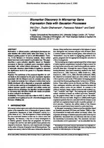
Machine learning in bioinformatics - Briefings in Bioinformatics [PDF]

8 MB - PDF

PDF - 8 Mb - Essilor

PDF (8 MB)

DownLoad PDF - Theoretical Biology & Bioinformatics

Integrating Machine Learning in Intelligent Bioinformatics - wseas.us

Machine learning in bioinformatics - Oxford Journals

a machine learning approach - Computational Systems Bioinformatics ...

Epigenetic machine learning: utilizing DNA ... - BMC Bioinformatics

Theoretical Immunology - Theoretical Biology & Bioinformatics

Machine-learning scoring functions for ... - BMC Bioinformatics

5 Machine Learning in Bioinformatics - Springer

Review PDF Machine Learning in Bioinformatics (Wiley ... - Google Sites

COS 511: Theoretical Machine Learning - cs.Princeton

COS 511: Theoretical Machine Learning - cs.Princeton

8 MB )

8 MB

PDF (8 MB) - Cell Press

PDF - 8 Mb - Internet Archive

articles - Theoretical Biology & Bioinformatics

Untitled - Theoretical Biology & Bioinformatics

Neural Networks and Machine Learning in Bioinformatics - Theory ...