THEORY AND EVALUATION OF A BAYESIAN MUSIC STRUCTURE EXTRACTOR Samer Abdallah, Katy Noland, Mark Sandler Michael Casey, Christophe Rhodes Centre for Digital Music Centre for Cognition, Computation and Culture Queen Mary, University of London Goldsmiths College, University of London Mile End Road, London E1, UK New Cross Gate, London SE14 6NW, UK
[email protected] [email protected] [email protected] [email protected] [email protected]
ABSTRACT We introduce a new model for extracting classified structural segments, such as intro, verse, chorus, break and so forth, from recorded music. Our approach is to classify signal frames on the basis of their audio properties and then to agglomerate contiguous runs of similarly classified frames into texturally homogenous (or ‘self-similar’) segments which inherit the classificaton of their consituent frames. Our work extends previous work on automatic structure extraction by addressing the classification problem using using an unsupervised Bayesian clustering model, the parameters of which are estimated using a variant of the expectation maximisation (EM) algorithm which includes deterministic annealing to help avoid local optima. The model identifies and classifies all the segments in a song, not just the chorus or longest segment. We discuss the theory, implementation, and evaluation of the model, and test its performance against a ground truth of human judgements. Using an analogue of a precisionrecall graph for segment boundaries, our results indicate an optimal trade-off point at approximately 80% precision for 80% recall. Keywords:
structure, segmentation, boundary, audio
1
INTRODUCTION
Methods for automatically segmenting music recordings into structural segments, such as verse and chorus, have immediate applications in music summarization, song identification, feature segmentation, feature compression and content-based music query systems. In order to evaluate an automatically-generated segmentation, however, we must develop an understanding of both the act of segmentation and the use to which a segmentation will be put. The notion of ‘a segment’ is intimately bound up with the notion of ‘a boundary’. It would be difficult to disPermission to make digital or hard copies of all or part of this work for personal or classroom use is granted without fee provided that copies are not made or distributed for profit or commercial advantage and that copies bear this notice and the full citation on the first page. c °2005 Queen Mary, University of London
420
agree with the proposition that, if a segment is (or is at least associated with) a temporal interval defined by its end-points, then these end-points must be ‘boundaries’ (in a sense which we intentionally leave undefined at this stage). Conversely, one might wish to argue that the interval between any two consecutive boundaries is a segment. Does this preclude the possibility that the interval between two non-consecutive boundaries is also a segment, perhaps on a larger scale? Furthermore, one could argue that, even if every boundary must be the start or end of some segment, the intervals between certain pairs of boundaries, such as the gap between two tracks on a CD, need not have the same ontological status as more substantive events, such as a verse or a drum solo. (To give a visual analogy, the space between objects is not necessarily an object.) Thus, we may conclude (a) that an enumeration of segments necessarily fixes all the boundaries, but (b) that the boundaries do not necessarily determine the segments without further information. In fact, the models we discuss in this paper are so constructed that the segments are indeed uniquely determined by the boundaries. Once we have come to a logically consistent position on the relationship between segments and boundaries, there remains the question of what criteria we are going to use to define and detect them. One approach, as exemplified by most the methods summarized below as well as our own contribution, is to consider some local properties of the signal (a sort of generalised ‘texture’) and assert that the segments are ‘texturally’ homogenous regions over which those properties are relatively constant. A corollary of this is that the boundaries can only appear where there is a change in the local texture. Whilst this has been the most common approach to segmentation from audio, it will fail in certain circumstances: consider a song which contains two separated verses in the first half but two consecutive verses in the second. If we successfully identify a local property which corresponds to ‘versiness’, that is, it is true whenever a verse is in progress, we will detect the first two verses but other two will be merged into one long verse, even if there are other features marking the boundary between the two. This approach is therefore incapable of detecting what one might call ‘unitary’ or ‘gestalt’ or ‘countable’ events; only that a certain type of event or process is occurring. Such distinctions are examined at great length in the literature on temporal logics and event calculi (eg,. Allen, 1984; Galton, 1987).
Assuming an approach based on textural similarity, a commonly used tactic is what one might call ‘atomisationclustering-agglomeration,’ which involves three steps: (1) divide the signal into a number of equal length fragments at the temporal resolution required for the boundaries and compute the value of the textural property (or feature tuple) for each fragment; (2) cluster the collection of property values ignoring the temporal relationships between the fragments to which they belong and thereby assign a class label to each fragment; (3) agglomerate runs of equally classified fragments into segments. In addition, the segments themselves can inherit the classification of their constituent fragments. This algorithm is liable to produce excessively fragmented segments if the clusters identified at stage (2) overlap, since fragments are classified without regard to the classifications of their temporal neighbours. This behaviour can be traced to a failure to encode our prior expectations about the durations of the segments we wish to detect. Indeed, this is an important factor in the segmentation process since there may be many valid segmentations of a piece of music, distinguished by their different time scales. In the following sections, we discuss previous work on audio segmentation, and present an atomisationclustering-agglomeration algorithm built around a probabilistic clustering model, which classifies all the segments found not just the ‘key’ segment or chorus. We evaluate our model against a ground truth of structural segmentations for a set of 14 popular song recordings, and discuss planned extensions to our system.
1.2
1.1
1.3
Segmentation by timbre
If broad spectral features are used to assess textural similarity, then we obtain what is essentially a timbre based segmentation resulting in timbrally homogenous segments. This is the approach taken by Aucouturier et al. (2005), who use mel frequency cepstral coefficients (MFCCs), which are selectivity of wide-band modulation in the source power spectrum whilst remaining relatively invariant to fine spectral structure. Foote (1999) proposed the dissimilarity matrix or Smatrix, containing a measure of dissimilarity for all pairs of feature tuples, for music structure analysis using MFCC features. With the initial analysis at 100 fragments per second, this means that a 3-minute song produces an 18000×18000 S-matrix. This extremely large, dense data object is the basis for the proposed methods, which are related to the recurrence plots discussed in Eckmann et al. (1987); for instance, Foote proposed that the chorus should be labelled as the longest ‘self-similar’ segment using a cosine distance measure and MFCC features. Logan and Chu (2000) proposed a method for summarization, also using MFCCs, employing both HiddenMarkov Models (HMMs) and threshold-based clustering methods, grouping features into key song segments. Peeters et al. (2002) propose a multi-pass clustering approach that uses both k-means and HMM-based clustering using multi-scale MFCC features. However, these studies provide no measure of performance for all segments in a song.
Segmentation by harmony
Some recent studies addressed the structure extraction problem in terms of harmonic rather than timbral features. For example Wakefield (1999) proposed chromagram features that represent the distribution of power spectrum energies among the twelve equal-temperament pitch classes based on A440, providing invariance to timbral changes in repeated segments. One desirable property of harmonic features is the possibility of implementing explicit transpositional invariance. Goto (2003) describes a system called RefraiD that locates repeated structural segments independent of transposition. The RefraiD system is able to track a chorus, for example, even if it modulates up a sequence of semitone key changes. The problem of chorus extraction was divided into four stages: computation of acoustic features and similarity measures; repetition judgement criterion; estimating end-points of repeated sections; and detecting modulated repetitions. This was the first work to explore the extraction of multiple structural segment types, i.e. verse and intro as well as chorus. The results for chorus detection were reported as accurate for 80 of 100 songs. However, the quality of the segmentation for non-chorus segments was not evaluated in that study. Dannenberg and Hu (2002) also describe a system that used agglomerative clustering with chroma-based features for music structure analysis of a small set of Jazz and Classical pieces. They do not report an evaluation of the methods over a corpus.
Segmentation by rhythm and pitch
Symbolic approaches to structure analysis attempt to identify the repeated thematic material in string-based music representations. Whilst these methods show much promise in identifying structure from score information, they are not well adapted for use in structure analysis from audio, largely due to the addition of significant uncertainty in audio representations. There has recently been some work on combined audio and symbolic representations, attempting to unify the different views of similarity. Maddage et al. (2004) describe a system in which a partial transcription is used to make decisions about structure, integrating beat tracking, rhythm extraction, chord detection and melodic similarity in a heuristic framework for detecting all segments in a song. They also propose using octave-scale rather than mel-frequency scale cepstral coefficients as pitch-oriented representation. The authors report 100% accuracy for detecting instrumental sections in songs, and report results for detection and labelling of verse, chorus, bridge, intro and outro sections. Similarly, Lu et al. (2004) describe an HMM-based approach to segmentation that used 1 a 12 th-octave constant-Q filterbank for pitch selectivity in addition to MFCC features. They report improved performance in segmentation for the constant-Q transform when used with MFCCs over use of MFCCs alone. Both of these methods used an S-matrix approach with an exhaustive search to find the best fit segment boundaries to a given objective function.
421
2
SEGMENTATION METHODS
Our segmentation algorithm follows the atomisationclustering-agglomeration approach described earlier, but several steps are required to compute the feature tuples, which are actually short-term histograms over state occupancy in a hidden Markov model (see section 2.1). These histograms are subsequently clustered using one of two methods described in sections 2.2 and 2.3. 2.1
Feature extraction
The processing chain begins with mono audio in WAVE format (IBM, 1991) and breaks it into a sequence of short overlapping fragments. This is then reduced to a sequence of discrete valued HMM states, going via a constant-Q log-power spectrum, normalisation to provide invariance to gross dynamics, and dimensionality reduction using PCA. The resulting 20-dimensional feature tuples represent the short-term power spectrum in a way comparable to the first 20 MFCCs, but using PCA results in the best (in a least-squares sense) low-dimensional approximation to the normalised log-power spectra. A Gaussianobservation HMM is then fitted to the sequence of PCA coefficients and the most probable state path inferred using the Viterbi algorithm 1 . Finally, a sequence of shortterm state occupancy histograms are formed using a sliding window. For example, if the HMM has 20 states and the histogram window covers 15 states, then each histogram has a total bin count of 15 distributed over 20 bins. 2.2
Pairwise clustering
The histograms resulting from the above processing steps inhabit a space which is not self-evidently Euclidean; clustering methods based on Euclidean feature values are therefore not trivially applicable. One way to proceed is to define an empirical dissimilarity measure between observed windowed state histograms with reasonable properties: histograms with the same distribution should be maximally similar, while those with no overlap should be maximally dissimilar. One such measure is the cosine dissimilarity measure as used by Foote (1999): using the vectors x and x′ to denote two l2 -normalized histograms, this is defined as dc (x, x′ ) = cos−1 (x · x′ ). As an alternative, we propose a symmetrization of the Kullback-Leibler divergence based on the interpretation of the histograms as summaries of data drawn from a multinomial probability distribution. With l1 normalized histograms x, x′ , we set dkl (x, x′ ) = PM 1 ′ ′ i=1 [xi log (xi /qi ) + xi log (xi /qi )] where qi = 2 (xi + ′ xi ) and M is the number of bins in the histograms. This can be interpreted as the sum of the KL divergences from either histogram to their mutual average q. These pairwise distances are then used in assigning frames to clusters using an algorithm due to Hofmann and 1
These preprocessing stages correspond closely to descriptors AudioSpectrumEnvelopeD, AudioSpectrumProjectionD, SoundModelDS and SoundModelStatePathD, defined in the MPEG-7 standard (Casey, 2001; ISO, 2002).
422
Buhmann (1997) which uses a form of mean-field annealing to minimise a cost function while avoiding local minima. 2.3
Histogram clustering
Since the data we wish to cluster are histograms representing a distribution over a discrete feature space (the HMM states), we may, following Puzicha et al. (1999), consider each underlying class to determine a probability distribution over the feature space. The observed histograms are then modelled as the result of drawing samples from one of these distributions. This leads quite naturally to a probabilistic latent variable model with an optimisable likelihood function. Assuming the existence of K underlying classes, the discrete distributions are parameterised by an M × K matrix A, such that Ajk is the probability of observing the jth HMM state in while in the regime modelled by the kth class. If C ∈ (1..K)L is the sequence of class assigments for a given sequence of histograms X ∈ NM ×L , then the overall log-likelihood of the model reduces to Hh =
L X M X K X
δ(k, Ci )Xji log
i=1 j=1 k=1
Xji Ajk
(1)
where L is the total number of histograms being considered, each of which relates to a certain fragment of the original signal. This cost function is optimised using a form of deterministic annealing as described by Puzicha et al. (1999), which is equivalent to expectation maximisation (Dempster et al., 1977) with a ‘temperature’ parameter which gradually falls to zero. The end result is a maximum a posteriori estimate for the class assignments C and the class-conditional distributions A.
3
EXPERIMENTS
We performed segmentations using the above-described methods on 14 popular music songs from Sony’s catalogue, which had been down-sampled to 11 kHz mono before being distributed to the MPEG-7 working group. The constant-Q spectrograms were computed every 200 ms over 600 ms frames and at a resolution of 81 -octave. The normalised log-power spectra were then encoded using their first 20 principal components. HMMs were trained with 10, 20, 40 and 80 states, and the state occupancy histograms were computed over windows of 15 states with a hop size of 1. Both clustering algorithms were applied with between 2 and 10 classes, resulting in segmentations with between 2 and 10 segment types. A sample segmentation, along with some of the intermediate results, is presented in figure 1.
4
EVALUATION
In order to evaluate the segmentations, they were compared against a ground truth consisting of annotations made by an expert listener, giving, for each ground truth segment, a start time in seconds, an end time in seconds and a label.
Nirvana:Smells Like Teen Spirit
80 state HMM histograms
pairwise(kl) : regions(0.2299,0.03494,0.8676), info(0.6786,2.069,0.6019)
histclust(mf) : regions(0.2369,0.06965,0.8467), info(0.5502,2.148,0.523)
annotation
0
50
100
150 time/s
200
250
Figure 1: A segmentation of a sample from the test set, comparing the results of dyadic clustering (using the symmetrized Kullback-Leibler distance) and the histogram clustering algorithm, both with 7 clusters. The constant-Q spectrogram is displayed in the top panel. The ‘ground truth’ annotations are displayed as different shades of grey for the different segment labels. Note how the fifth segment and its repeats have been split over two classes: in all cases, the same internal structure is visible. This effect was seen consistently in many of the songs in the test set. To make the comparison it is necessary to map the boundaries between segments back to the original continuous timeline on which the ground truth annotations are defined. Bearing in mind that the sequence of short-term histograms is defined on a discrete timeline which is itself derived via two framing operations from the original discrete time signal, this is not a trivial operation. Depending on how the fragment classification is interpreted, the boundary between two segments (essentially the ‘gap’ between two discrete time moments) could be mapped back to one of several points or intervals on the continuous timeline. We shall, for the time being, map the gap between two discrete moments back to the middle of the overlap between their respective continuous time intervals, which, at 15 HMM states, are 3.4 s long and overlap by 3.2 s. Having found times for the detected segment boundaries, we adapted the segmentation evaluation measure of Huang and Dom (1995). Considering the measurement i M as a sequence of segments SM , and the ground truth G j likewise as segments SG , we compute a directional Hami ming distance dGM by finding for each SM the segment j SG with the maximum overlap, and then summing the difP P i k j |S ference, dGM = S i ∩ S | where | · | dek M G SG 6=SG M notes the duration of a segment. We normalise dGM by the track length L to give a measure of the missed boundaries
m = dGM /L. Similarly, we compute dM G , the inverse directional Hamming distance, and a similar normalised measure f = dM G /L of the segment fragmentation. Note that these measures consider only the time intervals occupied by each segment, not the classifications of the segments. Plots of f and m against the number of clusters for our corpus are presented in figures 2 and 3. An alternative information-theoretic measure was also investigated in order to assess the how well the classification reflected the original segment labels. This involves ‘rendering’ the ground-truth segmentation into a discrete time sequence of numeric labels C0 , using the same discrete timebase as the sequence to be assessed, C1 , and then treating the the joint distribution over labels as a probability distribution. The two sequences are compared by computing the conditional ‘entropies’ H(C1 |C0 ) and H(C0 |C1 ). H(C0 |C1 ) measures the amount of groundtruth information ‘missing’ from the class assignments, while H(C1 |C0 ) measures the amount of ‘spurious’ information in the classfication, e.g. when several classes represent one segment type. The ‘mutual information’ I(C0 , C1 ) measures the information in the class assignments about the ground truth segment label, and is maximal when each segment type maps to one and only one class. In this case both H(C1 |C0 ) and H(C0 |C1 ) will be zero. We plot the mutual information for our segmentation methods in figure 4.
423
cosine distance
cosine distance
2
0.6
1
0.4 0.2
0 2
4
6 KL distance
8
10
0.6 0.4 0.2 0
2
4
6 8 histogram clustering
10
mutual information
false alarm rate
0
2
4
2
2
6 KL distance
8
10
4
6 8 histogram clustering
10
4
6 8 number of clusters
10
2 1 0
2 0.6
1
0.4 0.2 0
2
4
6 8 number of clusters
10
Figure 2: Rate of false detection f for all segmentation methods aggregated over our corpus. The four curves are for HMMs with 10, 20, 40 and 80 states; there is no strongly statistically significant difference between them.
0
Figure 4: Mutual Information (in bits) between ground truth and machine segmentation for our segmentation methods.
5 cosine distance
0.4 0.2
missing rate
0
2
4
2
2
6 KL distance
8
10
4
6 8 histogram clustering
10
4
6 8 number of clusters
10
0.6 0.4 0.2 0
0.6 0.4 0.2 0
Figure 3: Rate of true negative failure m for all segmentation methods aggregated over our corpus. As in figure 2, the four curves display the data for HMMs with different numbers of states.
424
CONCLUSIONS
Firstly, it is clear from the individual results that the approach we have taken in this paper, to a large extent independently of the details of the particular segmentation algorithm, has met with a degree of success. While no segmentation produced by our algorithm was perfect, some (represented in the top right corner of figure 5) are close to the ideal of the expert’s segmentation. We should note that the expert’s segmentation should not be taken as the Platonic truth: equally valid segmentations, depending on the application, can be formed at greatly different timescales; in addition, in real music there is often a degree of ambiguity, not reflected in the annotations, as to the exact point of transition between one segment and the next. A number of tendencies are visible in the results. Firstly, both the number of successfully detected boundaries and the number of false detections increase with the number of classes requested. This is unsurprising since, as the number of classes increases, each class becomes more selective, which tends to break up the segments and introduce more boundaries. Even if these were placed at random, this would increase both true and false positives. However, the increase in the mutual information measures shows that the extra classes are being put to good use as far as reflecting the annotated labels. Secondly, a close inspection of the individual segmentations shows that, in many cases, over-segmentation reveals the internal structure of the annotated segments in a consistent way; for example, in fig. 1, each repetition of
M. Casey. MPEG-7 sound-recognition tools. IEEE Trans. Circuits Syst. Video Techn., 11(6):737–747, 2001.
1
R. Dannenberg and N. Hu. Discovering musical structure in audio recordings. In Music and Artifical Intelligence: Second International Conference, Edinburgh, 2002.
0.8
0.6 1−f
A. P. Dempster, N. M. Laird, and D. B. Rubin. Maximum likelihood from incomplete data via the EM algorithm. Journal of the Royal Statistical Society, 39:1–38, 1977.
0.4
J.-P. Eckmann, S. O. Kamphorst, and D. Ruelle. Recurrence plots of dynamical systems. Europhysics Letters, 5:973–977, 1987.
0.2
0
0
0.2
0.4
0.6
0.8
1
1−m
Figure 5: Values of 1 − f , corresponding loosely to precision, plotted against values of 1 − m, analogous to recall, over all songs and segmentation methods presented. The optimal average tradeoff point is approximately (0.8,0.8). the fifth segment produces recognisably the same pattern of internal sub-segments. This effect is more pronounced when more classes are requested, resulting in distinctive pattern of several sub-segments on each repetition of the annotated segment type. Hence, the classified segmentation can be thought of as a sort of ‘abstract score’. Fragmentation also results if the clusters for two classes overlap in the histogram feature space. In this case, even a single frame in the middle of one segment which happens to look more another segment type will be misclassified. Intuitively, this occurs because we have not encoded any expectations of temporal coherence. In subsequent work, we have found that including an explicit prior on segment durations, to discourage very short segments, largely solves the fragmentation problem. Finally, in a bid to keep the parameter space tractable for this investigation, we have not discussed variations in the early stages in audio processing chain. In addition to the obvious parameters which could be varied, such as hop sizes or constant-Q resolution, the effects considering another representation, such as a chromagram, in place of or in addition to our constant-Q spectrum, warrant investigation.
ACKNOWLEDGEMENTS This research was supported by EPSRC grant GR/S84750/01 (Hierarchical Segmentation and Semantic Markup of Musical Signals).
REFERENCES J. Allen. Towards a general theory of action and time. Artificial Intelligence, 23:123–154, 1984. J.-J. Aucouturier, F. Pachet, and M. Sandler. The way it sounds : Timbre models for analysis and retrieval of polyphonic music signals. IEEE Transactions of Multimedia, 2005.
J. Foote. Visualizing music and audio using selfsimilarity. In ACM Multimedia (1), pages 77–80, 1999. A. Galton, editor. Temporal Logics and their Applications. Academic Press, London, 1987. M. Goto. A chorus-section detecting method for musical audio signals. In Proc. ICASSP, volume V, pages 437– 440, 2003. T. Hofmann and J. M. Buhmann. Pairwise data clustering by deterministic annealing. IEEE Transactions on Pattern Analysis and Machine Intelligence, 19(1), 1997. Q. Huang and B. Dom. Quantitative methods of evaluating image segmentation. In Proc. IEEE Intl. Conf. on Image Processing (ICIP’95), 1995. Multimedia Programming Interface and Data Specifications 1.0. IBM Corporation and Microsoft Corporation, August 1991. Information Technology – Multimedia Content Description Interface – Part 4: Audio. ISO, 2002. 15938-4. B. Logan and S. Chu. Music summarization using key phrases. In International Conference on Acoustics, Speech and Signal Processing, 2000. L. Lu, M. Wang, and H. Zhang. Repeating pattern discovery and structure analysis from acoustic music data. In 6th ACM SIGMM International Workshop on Multimedia Information Retrieval, October 2004. N. Maddage, X. Changsheng, M. Kankanhalli, and X. Shao. Content-based music structure analysis with applications to music semantics understanding. In 6th ACM SIGMM International Workshop on Multimedia Information Retrieval, October 2004. G. Peeters, A. L. Burthe, and X. Rodet. Toward automatic music audio summary generation from signal analysis. In International Symposium on Music Information Retrieval, 2002. J. Puzicha, T. Hofmann, and J. M. Buhmann. Histogram clustering for unsupervised image segmentation. Proceedings of CVPR ’99, 1999. L. Rabiner and B. H. Juang. Fundamentals of Speech Recognition. Signal Processing Series. Prentice Hall, Englewood Cliffs, NJ, 1993. G. H. Wakefield. Mathematical representation of joiint time-chroma distributions. In Advanced Signal Processing Algorithms, Architectures, and Implementations, volume 3807, IX, pages 637–645. SPIE, 1999.
425