Theory of Computing Systems

Theory Comput. Systems 34, 399–431 (2001) DOI: 10.1007/s00224-001-1034-2

Theory of Computing Systems ©

2001 Springer-Verlag New York Inc.

One-to-Many Embeddings of Hypercubes into Cayley Graphs Generated by Reversals L. Gardner,1 Z. Miller,2 D. Pritikin,2 and I. H. Sudborough1 1 Computer

Science Program, University of Texas at Dallas, Richardson, TX 75083, USA

2 Department

of Mathematics and Statistics, Miami University, Oxford, OH 45056, USA

Abstract. Among Cayley graphs on the symmetric group, some that have a noticeably low diameter relative to the degree of regularity are examples such as the “star” network and the “pancake” network, the latter a representative of a variety of Cayley graphs generated by reversals. These diameter and degree conditions make these graphs potential candidates for parallel computation networks. Thus it is natural to investigate how well they can simulate other standard parallel networks, in particular hypercubes. For this purpose, constructions have previously been given for low dilation embeddings of hypercubes into star networks. Developing this theme further, in this paper we construct especially low dilation maps (e.g., with dilation 1, 2, 3, or 4) of hypercubes into pancake networks and related Cayley graphs generated by reversals. Whereas obtaining such results by the use of “traditional” graph embeddings (i.e., one-to-one or many-to-one embeddings) is sometimes difficult or impossible, we achieve many of these results by using a nontraditional simulation technique known as a “one-to-many” graph embedding. That is, in such embeddings we allow each vertex in the guest (i.e., domain) graph to be associated with some nonempty subset of the vertex set of the host (i.e., range) graph, these subsets satisfying certain distance and connection requirements which make the simulation possible. 1. 1.1.

Introduction Hypercubes and Pancake Networks

Much recent attention has been given to n-dimensional interconnection networks having n! many processors, one for each permutation on n symbols [AK], [BHOS], [CB], [FMC],

400

L. Gardner, Z. Miller, D. Pritikin, and I. H. Sudborough

[HS], [MPS1], [MPS2], [NSK]. Such networks, usually defined as Cayley graphs on the symmetric group of order n!, often have a smaller diameter and fewer connections per processor than correspondingly large hypercubes. We consider the ability of some of these networks to simulate hypercubes efficiently. Specifically, we show how to embed hypercubes into them with very low dilation. We assume familiarity with basic concepts. Background not given here may be found in [L] and [MS1]. First we define the n-dimensional hypercube Q n , n ≥ 1, as follows. The vertex set V (Q n ) of this graph is the set of all binary strings of length n. The edge set E(Q n ) is the collection of all unordered pairs x y, where x, y ∈ V (Q n ) and x and y disagree in exactly one coordinate. We can view Q n as the graphical Cartesian product Q n = Q n 1 × Q n 2 × · · · × Q n m where the n i are any positive integers summing to n. Illustrations of Q 2 and Q 3 are given in Figure 3, where the vertices are indicated in the boxes, and the edges are indicated by lines joining appropriate pairs of boxed binary strings (the additional symbols in the drawing are explained later). As a special case, we let Q 0 be the graph having one vertex and no edges. Let 6n denote the group of all permutations on n symbols (with the operation of functional composition), i.e., the symmetric group of degree n. Let Tn be a set of generators for the group 6n . Then the Cayley graph determined by 6n and Tn , denoted by G(6n , Tn ), is the directed graph whose vertex set is 6n , with two permutations/vertices α, β connected by a directed edge from α to β if and only if β = α ◦ t for some generator t ∈ Tn . When the set Tn is closed under inverses this directed graph is symmetric, and thus each pair of oppositely oriented edges will be regarded as a single undirected edge, thereby allowing us to view G(6n , Tn ) as an undirected graph. We now introduce a family of Cayley graphs central to our study. For any integers 1 ≤ i < j ≤ n, let Rev[i, j] denote the permutation Ã ! 1 2 ··· i − 1 i i + 1 ··· j − 1 j j + 1 ··· n . 1 2 ··· i − 1 j j − 1 ··· i + 1 i j + 1 ··· n The permutations Rev[i, j] are called substring reversals because they can be thought of as reversing the substring between the ith and jth symbols inclusive. The special substring reversal Rev[1, j] is called a prefix reversal since it reverses the prefix between the first and jth symbols inclusive. Consider the set of generators An = {Rev[1, j]: j ≥ 2}, and let Pn denote the corresponding Cayley graph G(6n , An ), called the pancake network of dimension n. Our main goal is to construct efficient embeddings of hypercubes into pancake networks. As is standard, we typically regard 6n as the set of all n! arrangements of a set of specified and ordered symbols (where the ith symbol listed in an arrangement/permutation is regarded as the functional image of the ith symbol of the given order), and we regard the generators as acting upon these symbol strings by appropriately shuffling around the n symbols. For example, in P7 on the set of ordered symbols {A, B, C, D, E, F, G}, the vertices FDCBAGE and CDFBAGE are adjacent (via the generator Rev[1, 3]). Abusing our notation slightly, we often specify a set of ordered symbols by writing its elements as a string whose left to right order conforms to the ordering of the elements (e.g., the string ABCDEFG denotes the set {A, B, C, D, E, F, G} above).

One-to-Many Embeddings of Hypercubes into Cayley Graphs Generated by Reversals

401

We also consider so-called “burnt” networks related to Pn . The n-dimensional burnt pancake network [CB], [GP], [HS], denoted by BPn , is defined as follows. Given 62n on the symbols X 1 , X 2 , . . . , X 2n , the vertex set of BPn is the subgroup of 2n n! arrangements of those 2n symbols so that each symbol X 2i−1 appears consecutive to its paired symbol X 2i . The generator set for BPn is {Rev[1, 2i]: i ≥ 1}, thereby specifying the edges of the Cayley graph BPn . For an arbitrary symbol string S = Z 1 Z 2 · · · Z m let S r denote its “reverse,” i.e., S r = Z m Z m−1 · · · Z 1 . Using this notation we can view the vertex set of BPn as being all arrangements of n of the 2n symbols Y1 , Y2 , . . . , Yn , Y1r , Y2r , . . . , Ynr in which exactly one symbol appears from each of the symbol pairs {Yi , Yir }, where Yi denotes the string of two symbols X 2i−1 X 2i and Yir denotes its reverse. In this alternative notation each vertex of BPn is an arrangement of the n symbols Yi , each of which is also assigned an orientation, i.e., is in either ordinary or reversed mode. When vertices of BPn are regarded as arrangements of n “burnt”/oriented symbols instead of 2n nonoriented symbols we use the notation rev[i, j] (with a lower-case “r”) to stand for the generator that corresponds to Rev[2i − 1, 2 j] (the generator on 2n symbols). In particular, rev[1, i] acts to reverse the order and change the orientation of the first i burnt symbols (as opposed to Rev[1, i] reversing the order of the first i unburnt symbols). Thus each vertex of BPn can be thought of as a stack of n pancakes of various sizes, each burnt on one side, and the edges of BPn are present to indicate the option of grabbing the top i pancakes and turning this substack of i upside down, replacing them back on the rest of the stack. When such a substack is flipped, each of the i pancakes flipped changes orientation. The Cayley graph Pn has a similar interpretation, except that the pancakes have no orientation, i.e., turning a pancake over renders it indistinguishable from its previous state. Having defined these networks, we pause to mention some desirable features they possess. Vertices of Pn have degree n − 1, which is sublogarithmic relative to n!, the number of vertices. Its diameter is O(n) (see [HS] for the current best known implied constant), still sublogarithmic. Similarly, vertices of BPn have degree n and the diameter of BPn is O(n), which are sublogarithmic relative to 2n · n!, the number of vertices in BPn . By contrast, the hypercube Q n , being n-regular on 2n vertices and having diameter n, has degree and diameter which are logarithmic relative to the number of vertices. Thus each of the pancake and burnt pancake networks has a diameter which, relative to their number of vertices, is smaller than that of the hypercube while still retaining a smaller degree. From this limited viewpoint they are superior to the hypercube. Of course it takes much more for a network to prove itself nearly as useful as the hypercube, and the content of this paper is to show that it is possible to embed reasonably large hypercubes into these networks with very small dilation, a major step in showing that these networks can efficiently emulate hypercubes. Similar results have been shown for embedding hypercubes, binary trees, and cycles into “star networks” [BHOS], [MPS1], [MPS2], [K], another family of Cayley networks on the symmetric group. Since these networks are Cayley graphs, they are highly symmetric (e.g., vertex transitive), and their symmetries can be used to good effect in analyzing fault tolerance and broadcasting in these networks. Likewise, it is easy to see that Pn and BPn are recursive: the set of vertices in Pn (resp. BPn ) in which the last “pancake” is fixed induces a subnetwork isomorphic to Pn−1 (resp. BPn−1 ). For other literature concerning

402


pancake networks and related networks, see [CB], [GP], and [HS] concerning sorting, and [AQS], [BFP], [GVV], and [La] for broadcasting, routing, and other problems. 1.2.

Graph Embeddings and Simulation

As motivation for later definitions, we recall some related background on “traditional” (i.e., O(1) to 1) graph embeddings. Let G and H be two graphs representing two networks of processors, and let f : V (G) → V (H ) be a function mapping vertices of the “guest” graph G into those of the “host” graph H . Such a function f yields a model for studying simulations of G by H as follows. Consider an algorithm A designed to be run on G, which we wish to implement on H . The role of processor x in G will be played in the simulation by the processor f (x) in H . When a message between adjacent vertices x and y is sent in the execution of A on G, the equivalent message will be routed in the simulation of A on H along a designated path P(x, y) between f (x) and f (y) in H . We assume that at most one message can traverse any given edge during one step of any algorithm. We call f a graph embedding of G into H , though some authors may reserve that term for f together with the routing map associating a path P(x, y) with each edge xy ∈ E(G). There are costs associated with such a simulation. For example, a communication time of one step in sending a message across the edge x y in G is now “stretched” into taking a communication time proportional to the length of P(x, y) in H , thereby giving rise to a slowdown factor at least proportional to the maximum of the lengths of the paths P(x, y) over all edges x y in G. There may also be several messages routed through an edge e in H , only one of which can cross e in a given step of the simulation. Assuming f specifies these paths P(x, y) for each edge x y of G, the resulting congestion of f , defined as the maximum over all edges e in E(H ) of the number of paths P(x, y) containing e, contributes further to the slowdown. Let dist H (u, v) denote the distance between vertices u and v in a graph H . Now define the dilation of the map f by dilation( f ) = max{dist H ( f (x), f (y)): x y ∈ E(G)}. When the result of TG consecutive steps of a computation on G can be obtained by TH = s · TG consecutive steps of a computation on H (via the simulation afforded by f ), then we say that G can be simulated by H with slowdown s. Letting the load L of f be the maximum number of vertices of G mapped to any vertex of H , a result of [LMR] implies that a map f of load L, congestion c, and dilation d gives rise to a simulation of G by H with slowdown s = O(L + c + d). 1.3.

Our One-to-Many Model

In this paper we consider an alternative to traditional embeddings; that is, “one-to-many” embeddings from Q d to Pn , i.e., where the image of each vertex of Q d is now allowed to be an arbitrary nonempty subset of V (Pn ), these subsets being pairwise disjoint. Such embeddings are useful when a traditional embedding must have large dilation whereas a well-constructed one-to-many embedding can have low dilation (in a sense to be made precise below). We are also concerned with maximizing the size of the guest hypercube embedded into a given host pancake network. Let 2 X denote the power set of X . Given two networks G = (V, E) and H = (V 0 , E 0 ) 0 and an integer d, a function f : V → 2V − {∅} is called a one-to-many, dilation d


403

d

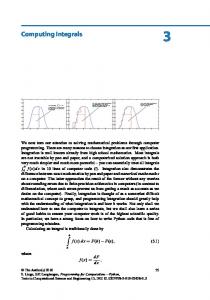
Fig. 1. A one-to-many embedding G ⇒ H seen as a map f : V (G) → 2V (H ) − ∅. It is required for each edge x y in G and each x 0 in f (x) that there exist at least one vertex yx0 0 in f (y) at distance at most d from x 0 in H . This is illustrated for the edge st, with s 0 ∈ f (s), ts0 0 ∈ f (t).

embedding of G into H if for every pair of vertices x, y in V the following two conditions are satisfied: (1) f (x) ∩ f (y) = ∅. (2) If x and y are adjacent in G, then for each x 0 ∈ f (x) there is a designated vertex yx0 0 ∈ f (y) for which dist H (x 0 , yx0 0 ) ≤ d. This definition is illustrated in Figure 1. To define congestion for one-to-many embeddings, suppose that for each x y ∈ E we have also specified a path P(x 0 , yx0 0 ) (resp. P(y 0 , x y0 0 )) in H of length at most d joining each pair of vertices x 0 ∈ f (x) and yx0 0 ∈ f (y) (resp. y 0 ∈ f (y) and x y0 0 ∈ f (x)). Such a collection of paths is called an edge routing for f . Then define the congestion of f to be the maximum, over all edges e ∈ E 0 , of the number of paths P(x 0 , yx0 0 ) containing e, as x y varies over all edges of E. A one-to-many embedding f of G into H gives rise to a simulation of G by H . A high-level view of how the simulation operates is as follows: (a) For every step of the algorithm A on G and every vertex x ∈ V (G), in the corresponding step of the simulation of A on H every vertex x 0 ∈ f (x) executes the same program and has the same input to that program as does x. This will be automatically accomplished by requiring that x 0 follow the same communication pattern as x in the following sense. (b) If x y is an edge in G and y sends a message to x at some step of the algorithm A, then in the simulation every vertex x 0 ∈ f (x) receives the same message (except for obvious changes in addressing) from the vertex yx0 0 ∈ f (y) in the corresponding step of the simulation of G by H . Thus (a) is implied by (b) since each such x 0 has been receiving the same messages at the corresponding stages during the simulation of A as x was receiving during the execution of A itself. Condition (a) stipulates that all processors in f (x) have the same information as x at corresponding stages. Thus when a processor x 0 ∈ f (x) receives information one

404


may naively anticipate a communication cost from having x 0 relay that information to other vertices in f (x) so that those vertices have the same information (as required by (a)). However, it is precisely the point of stipulation (b) that if a given x 0 ∈ f (x) receives information at a given simulation step, then every other x 00 ∈ f (x) receives the same information at that step. Hence there is no communication cost of this type. We discuss briefly the implementation of condition (b) and the resulting correspondence between steps of A on G and steps of its simulation on H . Again letting T = TG be the running time of algorithm A on G, take any time t, 1 ≤ t ≤ T . Consider all edges x y in G across which a message was sent, say from y to x, during the time interval [t − 1, t]. Now suppose we had a packet routing scheme Rt on H which for each pair x 0 ∈ f (x) and yx0 0 ∈ f (y) sends the packet from yx0 0 to x 0 which y sent to x during this time interval. The collection of such routing schemes Rt for all t then guarantees that condition (b) will be satisfied, and hence make our simulation possible, as follows. We initialize each vertex x 0 ∈ f (x) to be in the same state and possessing the same information and local program as x ∈ G at guest time t = 0. Let si be the time required to perform the routing Ri , 1 ≤ i ≤ TG . Then at host time s1 each x 0 ∈ f (x) is in the same state and has the same information as x has at time 1, having received exactly the same messages (from designated points yx0 0 for each neighbor y of x) as x received at the guest time interval [0, 1]. A simple induction Pt letting t −0 1 and t si each x ∈ f (x) play the roles of t = 0 and t = 1 above shows that at host time i=1 is in theP same state and has the same information as x had at guest time t. Thus, finally, T si (with T = TG ) each x 0 ∈ f (x) is in the same final state as x, so that H at time i=1 has simulated G. We can immediately obtain the slowdown and settle issues of synchronization in this implementation. Let s = max{si : 1 ≤ i ≤ TG }. We can achieve synchronization by agreeing to start the i 0 th round of routing Ri at host time (i − 1)s, even though some packets of the (i − 1)0 st round Ri−1 may have arrived at their destinations well before host time (i − 1)s. Concerning slowdown, observe that the message passing during the guest time interval [i − 1, i] is simulated by the i 0 th round of routing Ri requiring si ≤ s host time units. Hence TH = sTG , so we have a slowdown of s in our simulation. (We have ignored here the time required for local computations at host vertices x 0 ∈ f (x) since these times are identical to the local computation time for the corresponding guest vertex x ∈ f (x), and hence do not contribute to the slowdown.) 1.4. Other One-to-Many Models Our model is a direct adaptation to dilation d ≥ 1 of the one-to-many embedding model introduced in [F]. In that work the one-to-many map of dilation d = 1 (using other language) is defined and explored for embeddings involving hypercubes, grids, and complete graphs. A more general one-to-many simulation model was introduced in [KLM+ ]. In that model the graph H simulates G by creating and passing pebbles among its vertices, these pebbles representing computations and message passing in G. More precisely, for each vertex v ∈ V (G) and time t, 0 ≤ t ≤ TG , there is a vertex pebble (v, t) (representing the state of v at time t), and for t > 0 and any edge e of G an edge pebble (e, t) (these pebbles represent the message passed across edge e at time t). The goal of the simulation is to create a pebble (v, t) for all v and t, where at any step of the simulation a host vertex


405

h ∈ V (H ) may do the following operations: (1) copy a single edge pebble that it contains, (2) send a single edge pebble to a neighbor in H , (3) create either a vertex pebble (v, t) or edge pebble (e, t) for some edge e leaving v in G if h contains the pebbles (v, t − 1) and (ei , t − 1), 1 ≤ i ≤ k, where ei are the edges of G going into v. We examine the generality in such a simulation. Observe that multiple copies of a pebble (v, t) can be created throughout the host H . This redundancy is in effect a simulation of guest vertex v at guest time t at multiple host vertices in H ; i.e., a oneto-many simulation of G by H . However, this simulation is dynamic in the following sense. For any host time τ, 0 ≤ τ ≤ TH , let H (v, τ ) be the set of vertices of H which at host time τ play the role of v, in the sense of creating at time τ a pebble (v, t) for some t. Further, let H (v) = ∪0≤τ ≤TH H (v, τ ), the set of all vertices in H which at any point in the simulation play the role of v. Then operations (1)–(3) allow the possibility H (v, τ ) 6= H (v, τ 0 ) for τ 6= τ 0 . That is, the set of host vertices simulating a given guest vertex v can vary with host time. These operations further allow the possibility of nonempty pairwise and arbitrary k-fold intersections among the sets H (v); in effect allowing a given host vertex h to play the role of k ≥ 1 different guest vertices for arbitrary k during the simulation, though during any single step h can play the role of only one guest vertex. In our model we disallow the analogous possibilities, i.e., the variation with time of the set H (v, τ ) and the nonempty intersection of sets H (v). This is because in our model the set of vertices of H playing the role of v ∈ V (G) is fixed to be f (v) (where f is our one-to-many map) independent of time, and f (v) ∩ f (w) = ∅ for v 6= w by definition of f . This dynamic redundancy in [KLM+ ] makes possible the construction of small slowdown simulations, in some cases even in the presence of high dilation. Thus, as one example, it is shown that an N -vertex butterfly B can simulate an N -vertex mesh M with O(1) slowdown despite the fact that a one-to-one embedding M → B must have dilation Ä(log(N )) [BCH+ ]. Several other upper and lower bounds on the slowdown of simulations are derived involving trees, multidimensional grids, and hypercube-derived networks such as the butterfly and shuffle exchange. The simulations underlying the upper bounds are static in that they satisfy H (v) ∩ H (w) = ∅, for v 6= w. The lower bounds (with one exception) apply to any simulation based on their model, in particular to ones allowing the dynamic possibilities H (v) ∩ H (w) 6= ∅ and H (v, τ ) 6= H (v, τ 0 ) described in the preceding paragraph. Other simulations based on one-to-many embeddings can also be found in [M1], [M2], and [MW]. In [M2] a bounded degree network H on N 1+ε vertices is constructed, with ε > 0 fixed but arbitrarily chosen, that can simulate with O(1) slowdown any bounded network on N vertices. In [M1] it was shown that there is no N vertex bounded degree network which can simulate all N vertex bounded degree networks with slowdown less than Ä(log(N )/ log(log N )). 1.5. Our Results The focus of this paper is on embedding hypercubes into pancake (and related) networks with very small dilation D, i.e., 1 ≤ D ≤ 4. Simultaneously we aim to keep the

406


expansion of these embeddings low, i.e., we want to make the guest hypercube as large as our methods allow, given the host pancake network. To achieve such results, a one-to-many embedding model seems necessary. We do not know how to construct one-to-one maps of such small dilation and reasonably low expansion for these networks. Indeed, we know that there is no dilation D = 1 one-toone map Q 2 → Pn for any n, and hence no such map Q d → Pn for d ≥ 2. The relation between d and n in the one-to-many maps of Q d into Pn (of the required dilation) which we construct is summarized in the table of Section 6. As D increases from 1 to 4, the dimension d √ of the hypercube we are able to embed into Pn with dilation D increases from d = 2( n) to d = n log(n) − (2 + o(1))n. Concerning the congestion of our embeddings, in the case D = 1 we trivially have congestion 1, using the path x 0 − yx0 0 (of length 1) in Pn joining the images of the edge xy in Q d . When D = 2 we will show a natural routing of images of edges with a congestion of 4. Hence in these two cases, having constant dilation and congestion, a slowdown of O(1) follows in the resulting simulation of Q d by Pn . For the cases D = 3 and D = 4 we have congestion Ä(log(N ) − log(log(N ))) and Ä(log(N )), respectively, forced by the ratio of the vertex degree in the guest Q d to the vertex degree in the host Pn . Finally, we note that it can be misleading to look at our results purely from the standpoint of the slowdown in the simulation to which they give rise. The O(1) slowdown in the cases D = 1 and D = 2, while certainly a desirable consequence, is in a real sense a weaker result than the dilation 1 or 2 map from which it arises. Indeed, if constant factors were unimportant, then a simulation of any constant dilation K and constant congestion c would yield a O(1) slowdown. Again we emphasize that our goal here is to explore the one-to-many mapping technique of [F] as a tool for constructing low dilation maps of reasonably low expansion among potential computation networks. 1.6. Additional Notation and Preliminary Results d

We write G ⇒ H to indicate that there exists a one-to-many dilation d embedding of G d

into H . We write G → H to indicate that there exists a one-to-one dilation d embedding of G into H , i.e., the traditional sort of embedding. We write G ⊆ H to indicate that there exists a one-to-one dilation 1 embedding of G into H , i.e., that G is isomorphic to a subgraph of H . A one-to-many dilation d embedding of G = (V, E) into H = (V 0 , E 0 ) is essentially a particular kind of relation R from V to V 0 , where xRy if and only if y ∈ f (x). Requirement (1) above stipulates that each element of V 0 is related to exactly one or zero elements of V , so that the inverse relation of R, when restricted to the range of R, is in fact a function. Therefore it is typically convenient to specify a one-to-many dilation d embedding of G into H by specifying the range R ⊆ V 0 of R and specifying the function g: R → V corresponding to the inverse of R, thereby implicitly specifying the “actual” embedding by f (x) = {y ∈ V 0 : g(y) = x}, where R is the part of H actually used in embedding G within it (in fact R = ∪x∈V f (x)). The function g and related notation are given as follows. A co-embedding of dilation d of G = (V, E) into H = (V 0 , E 0 ) is a pair (R, g) where ∅ 6= R ⊆ V 0 and g: R → V is an onto function such that for every y ∈ R and neighbor x 0 of g(y) in G there exists some y 0 ∈ R such that g(y 0 ) = x 0 and dist H (y, y 0 ) ≤ d. Since R is the domain of g we usually refer to g as being the co-


407

embedding, R understood implicitly. By the comments above we see that there exists a one-to-many dilation d embedding f of G into H if and only if there exists a dilation d co-embedding g of G into H . Cartesian products of graphs will often appear, and it is convenient to have some special language for them in the context of one-to-many embeddings. First recall that for graphs G 1 , G 2 , . . . , G n the Cartesian product graph G = G 1 × G 2 × · · · × G n has vertices and edges given by V (G) = {v: v = (v1 , v2 , . . . , vn ), vi ∈ G i for 1 ≤ i ≤ n},

and

E(G) = {vw: v, w ∈ V (G), and for some r we have vi = wi for i 6= r while vr is adjacent to wr in G r }. d

Many of the embeddings we construct are of the type G ⇒ H where G is such a product. d (This type of embedding naturally includes maps Q n ⇒ H since we can view Q n as the n-fold product K 2 × K 2 × · · · × K 2 .) Using the equivalence above we specify such an embedding by constructing a dilation d co-embedding of G into H . To do this we typically first give a function g: R → V (G), and second show that the defining condition for a dilation d co-embedding is satisfied by this function. To facilitate this second step in the case where G is the graph product above, the following language will be useful. Let z ∈ R and let the i 0 th coordinate of g(z) be the vertex y of G i . With d understood by context, to toggle the i 0 th coordinate of z is to show that, for any vertex y 0 ∈ G i adjacent to y in G i , there exists z 0 ∈ R with dist H (z, z 0 ) ≤ d such that g(z) and g(z 0 ) disagree only in the i 0 th coordinate, and that the i 0 th coordinate of g(z 0 ) is y 0 . Note the slight abuse of this notation in that the coordinate in question is literally the i 0 th coordinate of g(z) rather than of z. Note too that when a factor of G is a complete graph, i.e., G i = K m i , then the vertex y 0 is allowed to be any vertex of G i , since any two vertices of such a G i are joined by an edge. When each factor of G is K 2 , i.e., G = Q n , then each of the coordinates of g(z) can be taken to be either 0 or 1 so we then speak of toggling the i 0 th bit of z. From the definition of adjacency in Cartesian products, the ability to toggle the i 0 th coordinate of z for all i says that for any neighbor u 0 of g(z) in G, there exists z 0 ∈ R such that dist H (z, z 0 ) ≤ d and g(z 0 ) = u 0 . So showing how to toggle the i 0 th coordinate of z for any z ∈ R and any i, 1 ≤ i ≤ n, is really proving that the proposed map g is indeed a dilation d co-embedding of the Cartesian product G into H . Thus throughout this paper we routinely and implicitly specify one-to-many dilation d embeddings of such products G into H by specifying a map g: R → V (G), R ⊆ V (H ), along with a demonstration of how to toggle each of the n coordinates of z for each z ∈ R. The one-to-many embedding thereby specified will be a one-to-one embedding if and only if g is one-to-one. Some of these notions are illustrated in the following proof. Let ⊕ denote the bitwise modulo-2 sum operation for bit strings, and let “;” denote the concatenation of strings. So, for example, letting A = 1100 and B = 1010, we have A ⊕ B = 0110 and A; B = 11001010. Lemma 1.

For any m, n, d ≥ 1: d

d

d

d

d

d

d

d

(a) If Q m ⇒ Pn , then Q m+1 ⇒ P2n . If Q m ⇒ BPn , then Q m+1 ⇒ BP2n . (b) If Q m → Pn , then Q m+1 → P2n . If Q m → BPn , then Q m+1 → BP2n .

408


Proof. Let (R 0 , g 0 ) (resp. (R 00 , g 00 )) be a dilation d co-embedding of Q m into Pn , where 6n is viewed as permutations of the symbol string X 1 X 2 · · · X n (resp. X n+1 X n+2 · · · X 2n ). With 62n being permutations of X 1 X 2 · · · X 2n , let R = {α; β r : (α ∈ R 0 and β ∈ R 00 ) or (α ∈ R 00 and β ∈ R 0 )}. Let h: R 0 ∪ R 00 → Q m be defined by h(α) = g 0 (α) if α ∈ R 0 and h(α) = g 00 (α) if α ∈ R 00 . Then define g: R → Q m+1 by g(α; β r ) = (h(α) ⊕ h(β)); B, where B = 0 if α ∈ R 0 and B = 1 if α ∈ R 00 . We show that g is a dilation d coembedding. To toggle the (m + 1)th bit of α; β r we apply Rev[1, 2n] to obtain β; α r , noting that g(α; β r ) and g(β; α r ) differ in exactly the (m + 1)th bit. To toggle the ith bit of α; β r for 1 ≤ i ≤ m when α ∈ R 0 (resp. α ∈ R 00 ) we apply the same sequence of d or fewer generators that serve to toggle the ith bit of α relative to the co-embedding g 0 (resp. g 00 ). Having shown that any bit of α; β r can be toggled via a path of length d or less in P2n , we have proven the first part of (a). The proof of the second part of (a) is essentially the same. As for (b), the further supposition that co-embeddings g 0 and g 00 are one-to-one is the same as supposing the conditions in the premise of (b), and since the resulting g constructed is then one-to-one we have also proven (b). We now introduce some additional related Cayley graphs on 6n . Let (i, j) denote the permutation which transposes symbols i and j. Consider the following sets of generators for 6n : Bn Cn Dn En

= = = =

{(i, j): 1 ≤ i < j ≤ n}, {(1, j): j ≥ 2}, {Rev[i, j]: 1 ≤ i < j ≤ n}, where Rev[i, j] is defined as above, {Cyci : i ≥ 2}, where µ ¶ 1 2 3 ··· i − 1 i i + 1 ··· n , Cyci = i 1 2 ··· i − 2 i − 1 i + 1 ··· n

Fn = {Cyci : i ≥ 2} ∪ {(Cyci )−1 : i ≥ 2}. The permutations Cyci or (Cyci )−1 are called prefix cycles. Each of An , Bn , Cn , Dn , Fn happens to be closed under the inverse operator, so their Cayley graphs listed below are regarded as undirected graphs. G(6n , Bn ) is called the transposition network of dimension n, G(6n , Cn ) is called the star network of dimension n, G(6n , Dn ) is called the substring reversal network of dimension n, denoted by SSRn , and G(6n , Fn ) is called the cycle prefix network of dimension n, denoted by CPn . The first three of these networks can be found in [AK], and CPn can be found in [FMC]. The directed Cayley graph G(6n , E n ) is called the dicycle prefix network of dimension n, denoted by DCPn . In a manner entirely analogous to how BPn was defined, the n-dimensional burnt substring reversal network, denoted BSSRn , has a generator set {Rev[2i − 1, 2 j]: 1 ≤ i ≤ j ≤ n} = {rev[i, j]: 1 ≤ i ≤ j ≤ n}. Of the networks in this paper, only DCPn is a directed graph, the others being viewed as undirected by the convention described previously. The following examples illustrate how these Cayley graphs may be viewed as arrangements of ordered symbols joined by edges corresponding to suitable generators: In SSR7 on the ordered symbol set ABCDEFG there exists a path of length 2 given by EGBDFCA to EGFDBCA to ACBDFGE (applying generators Rev[3, 5]) followed


409

by Rev[1, 7]). Generally observe that in SSRn two symbol strings X, Y are adjacent if and only if X, Y are expressible in the forms X = A; B; C and Y = A; B r ; C where the substring B must have at least two symbols, and substrings A, C are possibly empty. In CP7 on the ordered symbol set ABCDEFG there exists a path of length 2 given by EGBDFCA to GBDFECA to AGBDFEC (applying generators (Cyc5 )−1 and Cyc7 ). Again observe in general that in CPn two symbol strings X, Y are adjacent if and only if X, Y are expressible in the forms X = a; B; C and Y = B; a; C where a is a single symbol and where the substring C is possibly empty. In Pn two symbol strings X, Y are adjacent if and only if X, Y are expressible in the forms X = A; B and Y = Ar ; B where the substring B is possibly empty. These pancake-like networks are useful models for research in computational biology. Thus, for example, if a segment of a DNA strand were to become detached, then flip and reattach itself in reverse orientation, then the corresponding “mutation” can be viewed as a neighboring vertex of the original strand in a substring reversal network. The table at the end of the paper summarizes the various reversal networks defined above. As for how some of the Cayley graph networks defined above relate to one another, we have the following. Theorem 1. 2

(a) CPn → Pn . 3 (b) SSRn → Pn . 3 (c) BSSRn → BPn . Proof. In each case the embedding f is simply the identity map. Thus to verify that each is a dilation d embedding it suffices to show that each generator in the “guest” network is a composition of d or fewer generators in the “host” network. For (a), Cyci = Rev[1, i] ◦ Rev[1, i − 1] and (Cyci )−1 = Rev[1, i − 1] ◦ Rev[1, i]. For (b), Rev[i, j] = Rev[1, j] ◦ (Rev[1, j −i +1]◦Rev[1, j]). For (c), rev[i, j] = rev[1, j]◦(rev[1, j −i +1]◦rev[1, j]).

For the rest of the paper we concentrate on constructing efficient low dilation embeddings of hypercubes into pancake networks and their relatives.

2.

Dilation 1 Embeddings

We begin with a theorem concerning embeddings of hypercubes and other Cartesian products of cliques into dicycle prefix networks. Theorem 2. 1

(a) For all m ≥ 1, Q m ⇒ DCP2m .

410

L. Gardner, Z. Miller, D. Pritikin, and I. H. Sudborough 1

(b) For m 1 , m 2 , . . . , m n ≥ 2, K m 1 × K m 2 × · · · × K m n ⇒ DCPs where s = 1

m 1 + m 2 + · · · + m n . Thus G 1 × G 2 × · · · × G n ⇒ DCPs where each G i is an arbitrary graph of order m i . Proof. For any permutation π in R = 62m of the 2m symbols X 1,0 X 1,1 X 2,0 X 2,1 · · · X m,0 X m,1 , let g(π) = b1 b2 · · · bm , where bi = 0 or 1 depending upon which appears first (leftmost) in π among the symbols X i,0 and X i,1 . To toggle the ith bit, apply the appropriate cyclic shift to bring to the front whichever of X i,0 and X i,1 occurs after the other. This reverses their order and leaves every other pair X k,0 and X k,1 in the same relative order, so g is a dilation 1 co-embedding, proving (a). The proof of (b) is similar, involving the s symbols X 1,0 X 1,1 · · · X 1,m 1 −1 · · · X n,0 X n,1 · · · X n,m n −1 , where bi is determined by the leftmost second subscript k appearing in a symbol X i,k . The second part of (b) follows from G i ⊆ K m i . A corollary of Theorem 2(b) is that the n-dimensional r -ary hypercube (K r )n has a one-to-many dilation 1 embedding into DCPnr . Lemma 2. (a) If Q m ⊆ BSSRk , then Q m+2 ⊆ BSSRk+1 . (b) Q m−1 ⊆ BSSRm for each positive integer m, via an embedding f 00 such that no two vertices f 00 (x), f 00 (y), x 6= y, are the same m-symbol string when regarded as strings in SSRm , i.e., with orientations suppressed. (c) Q m−1 ⊆ SSRm . Proof. Suppose f : Q m → BSSRk embeds Q m as a subgraph of BSSRk , with 6k being defined on the k burnt symbols X 1 X 2 · · · X k . Define f 0 : Q m+2 → BSSRk+1 as follows, with BSSRk+1 being on the burnt symbols X 1 X 2 · · · X k A. For x ∈ Q m let f 0 (x; 00) = f (x); A, let f 0 (x; 01) = f (x); Ar , let f 0 (x; 10) = Ar ; [ f (x)]r , and let f 0 (x; 11) = A; [ f (x)]r . It is straightforward to verify that f 0 embeds Q m+2 as a subgraph of BSSRk+1 , proving (a). For (b) we proceed by induction on m, noting that Q 0 has such an embedding in BSSR1 , serving as a basis step. Suppose f m00 is such an embedding of Q m−1 in BSSRm , with 00 : Q m → BSSRm+1 as follows, with 6m on the m burnt symbols X 1 X 2 · · · X m . Define f m+1 00 (x; 0) = f m00 (x); A and 6m+1 on the burnt symbols X 1 X 2 · · · X m A. For x ∈ Q m−1 let f m+1 00 00 r 00 r let f m+1 (x; 1) = A ; [ f m (x)] . It is straightforward to verify that f m+1 is an embedding satisfying (b), completing the induction. Suppressing the orientations of the burnt symbols in each f 00 (x), we see that f 00 induces a dilation 1 embedding of Q m−1 in SSRm . Lemma 2(b) fuels the proof of the following lemma, showing how one can combine various dilation 1 embeddings of hypercubes into SSR networks to produce an embedding of a larger hypercube into a larger SSR network, the dimension of the large hypercube now embedded being a bit larger than might otherwise be anticipated.


Lemma 3.

411

If Q ni ⊆ SSRki for i = 1, 2, . . . , m, then Q m−1+6ni ⊆ SSR6ki .

Proof. Let f 00 : Q m−1 → BSSRm be the embedding from Lemma 2(b), relative to the m burnt symbols Y1 Y2 · · · Ym . Let f i : Q ni → SSRki be dilation 1 embeddings as assumed, where each SSRki is on the symbols X i,1 X i,2 · · · X i,ki . Then our dilation 1 embedding f : Q m−1+6ni → SSR6ki is defined as follows. For x ∈ Q m−1 and xi ∈ Q ni let f (x; x1 ; x2 ; . . . ; xm ) be the string resulting from f 00 (x) by replacing each Yi in f 00 (x) by f i (xi ), each Yir in f 00 (x) by [ f i (xi )]r . In other words, f (x; x1 ; x2 ; . . . ; xm ) is the concatenation of substrings f 1 (x1 ), f 2 (x2 ), . . . , f m (xm ) formed by arranging them in the order determined by f 00 (x), and reversing those f i (xi )’s for which Yi appears reversed in f 00 (x). To see that f is a dilation 1 embedding, observe that if x, y are adjacent in Q m−1 , then f (x; x 1 ; x2 ; . . . ; xm ) and f (y; x1 ; x2 ; . . . ; xm ) differ by a substring reversal which reverses the concatenation of several substrings made up of Yi ’s and/or (Yir )’s (i.e., one can always toggle any one of the bits corresponding to x), and if xi , yi are adjacent in Q ni , then f (x; x 1 ; x2 ; . . . ; xi ; . . . ; xm ) and f (x; x1 ; x2 ; . . . ; yi ; . . . ; xm ) differ by a substring reversal internal to the substring f i (xi ) or [ f i (xi )]r of f (x; x1 ; x2 ; . . . ; xi ; . . . ; xm ) (i.e., one can always toggle any one of the bits corresponding to xi ). Theorem 3. (a) If Q n ⊆ SSRk , then Q n+1 ⊆ SSRk+1 . (b) If Q n ⊆ SSRk , then Q mn+m−1 ⊆ SSRmk . (c) Q 2n +2n−2 −1 ⊆ SSR2n . Proof. Claim (a) follows from Lemma 3 via the parameters m = 2, n 1 = 0, n 2 = n, k1 = 1, k2 = k. Claim (b) follows from Lemma 3 via the parameters m, n 1 = n 2 = · · · = n m = n, k1 = k2 = · · · = km = k. Claim (c) is proven by induction on n. The basis case n = 2 is handled by the embedding illustrated in Table 1. Assuming that Q 2n +2n−2 −1 ⊆ SSR2n , then from (b) with m = 2 we have Q 2(2n +2n−2 −1)+2−1 ⊆ SSR2n+1 , i.e., Q 2n+1 +2n−1 −1 ⊆ SSR2n+1 , completing the induction. Since Q m has 4-cycles and Pn does not, it is never possible to embed Q m into Pn for m > 1 via a one-to-one dilation 1 embedding. Hence we consider building such embeddings by the one-to-many technique. Toward this end, the following “exponent” and “block” terminology is convenient for describing certain sets of vertices in Pk . Table 1. A dilation 1 embedding of Q 4 into SSR4 , showing Q 4 ⊆ SSR4 . 0000 0001 0010 0011 0100 0101 0110 0111

1234 2134 1243 2143 1324 2314 1423 2413

1000 1001 1010 1011 1100 1101 1110 1111

4321 4312 3421 3412 4231 4132 3241 3142

412


Suppose Pk is defined on the symbol set A1 A2 · · · Ak−r B1 B2 · · · Br . We then write At as shorthand for a string composed of t many distinct A’s. Every string x ∈ V (Pk ) is of the form x = W0 (x); D1 (x); W1 (x); D2 (x); W2 (x); . . . ; Dr (x); Wr (x), or for brevity x = W0 ; D1 ; W1 ; D2 ; W2 ; . . . ; Dr ; Wr when x is understood by context, where each Wi is a substring of distinct A’s such that W0 ; W1 ; . . . ; Wr is a permutation of A1 A2 · · · Ak−r and D1 D2 · · · Dr is a permutation of B1 B2 · · · Br . Thus the Wi ’s are the maximal substrings of consecutive A’s in x, and for any integer k ≥ 1 the string Wk is the one immediately following the kth B symbol from the left. The substring W0 is called the front string of x, and for each i ≥ 1 substring Wi is called a block of x, and for i ≥ 0 we let N x (i) denote the number of A symbols in Wi . Given a sequence of nonnegative integers x0 , x1 , . . . , xr summing to k −r , we let A X 0 BA X 1 B · · · BA Xr denote the set of vertices in Pk for which N x (i) = xi for all i. An unsubscripted B or A symbol with no exponent refers to a single symbol of the given type. As an example, the string A1 A4 B3 A3 B2 A8 A5 B1 A6 A7 A2 belongs to the collection of vertices A2 BABA2 BA3 in the pancake network P11 having the symbol set {Ai : 1 ≤ i ≤ 8} ∪ {Bi : 1 ≤ i ≤ 3}. Our main theorem in this section is Theorem 4, in which we give dilation 1 one-tomany embeddings of hypercubes into pancake networks. Theorem 4 is a special case of the more general Lemma 4, the latter capturing the method underlying the construction of these embeddings. So as to motivate the ideas behind Lemma 4, we next prove a claim whose value is in that its proof will help with understanding Lemma 4. This claim happens to concern dilation 2 (not dilation 1) one-to-many embeddings, yet it prepares the ideas leading to Lemma 4. Claim. Let G 1 , G 2 , . . . , G m be graphs, and let νi = |V (G i )| ≥ 2. Suppose for each i that Ii is an interval of νi many positive integers, the largest element Mi in each Ii Pm 2 satisfying Mi ≥ νi − 1. Let M = i=1 Mi . Then G 1 × G 2 × G 3 × · · · × G m ⇒ Pm+M . Proof. Let Pm+M be defined on the symbol set A1 A2 · · · A M B1 B2 · · · Bm . We assume that the vertex set of each G i is {0, 1, 2, . . . , νi − 1}. This choice of vertex set for G i is convenient since vertices of G = G 1 × G 2 × G 3 × · · · × G m are then merely m-tuples of whole numbers, allowing the possibility that we specify a particular coordinate of a desired vertex by a simple count. We construct a co-embedding g for a dilation 2 one-tomany embedding of G into Pm+M . Let the domain R of g be the set of vertices in Pm+M of the form A x0 BAx1 BAx2 B · · · BAxm for which xi ∈ Ii for i = 1, 2, . . . , m. That is, a string x ∈ V (Pm+M ) is in R if and only if the length of block Wi is an element of interval Ii for i = 1, 2, . . . , m. Note that R is nonempty, since its subset A0 BA M1 BA M2 B · · · BA Mm is nonempty. The rule for the function g is given by g(x) = (M1 − N x (1), M2 − N x (2), . . . , Mm − N x (m)). That is, the ith coordinate of g(x) is the amount by which N x (i) falls short of its maximum allowable value Mi . Thus the νi consecutive integer values in Ii correspond (in reverse order) to the νi possible values of the ith coordinate of a vertex in G.


413

To show that g is a dilation 2 co-embedding as claimed, we show for each y ∈ R how to toggle any coordinate of y. So let x 0 be any neighbor of x = g(y) in G, and we show that there exists some y 0 ∈ R such that g(y 0 ) = x 0 , where y 0 can be obtained from y using at most two prefix reversals. Suppose that the sole coordinate in which x and x 0 differ is the ith coordinate. Let c ≤ νi − 1 be the ith coordinate of x 0 , where we recall that Mi − N y (i) 6= c is the ith coordinate of x. The following sequence of two prefix reversals illustrates how such a y 0 can be found starting with arbitrary y, and the reader may find this useful in following the remainder of the proof: y = W0 BW 1 BW 2 B · · · BW i−1 BW i B · · · Wm

(abbreviating Wi (y) as Wi

throughout) r r BW i−2 B · · · BW r1 BW r0 Wi B · · · Wm → z = BW i−1

(note that W0r Wi = A Nz (i)−(Mi −c) ; A Mi −c ) → y 0 = A Nz (i)−(Mi −c) BW 1 BW 2 B · · · BW i−1 BA Mi −c B · · · Wm . As our first step, we apply to y the prefix reversal which reverses all symbols to the left of Wi , letting z be the string thus obtained. Blocks W1 (y) through Wi−1 (y) of y appear in z internally reversed and collectively in reverse order (as the blocks Wi−1 (z) through W1 (z) of z, respectively), and the front string W0 (y) of y appears in z now merged with a new block Wi P (z) consisting of N y (0) + N y (i) many A symbols. Now, Wi (y) to form P m N (k) = N y (0) = M − m k=1 y k=1 (Mk − N y (k)) ≥ Mi − N y (i), so Wi (z) contains at least Mi many A symbols. Since Mi ≥ vi − 1 ≥ c, we have that Mi − c is a nonnegative integer. As our second step, we apply to z the prefix reversal which reverses all symbols to the left of the rightmost Mi − c symbols of Wi (z) (i.e., affecting all the leftmost Nz (i) − (Mi − c) many symbols of Wi (z)), letting y 0 be the string thus obtained. It is easy to see that g(y 0 ) = x 0 as desired, since in transforming z to obtain y 0 we have restored blocks W1 through Wi−1 of y as appearing as the first i − 1 blocks from left to right in y 0 , we have left undisturbed blocks Wi+1 through Wm of y, and have rendered the ith block from the left in y 0 as having precisely Mi − c many A symbols so that the ith coordinate of g(y 0 ) is indeed c. We summarize this proof as an interchange of A symbols between blocks P and the front string. The front string W0 acted as a “reservoir” composed of N y (0) = m k=1 (Mk − N y (k)) many A symbols, a supply sufficiently large that (should the need arise) we could use the A’s in W0 to increase the values N y (1), N y (2), . . . , N y (m) to their “maximum” allowed values M1 , M2 , . . . , Mm , respectively. Should we wish to reduce a value N y (i) we need only transfer some of the A symbols of Wi into the front string. In the span of two prefix reversals we saw that we could leave undisturbed all blocks other than Wi and in the process change the value of N x (i) to any desired value in Ii , thereby proving that we could alter any one coordinate of g(y) to any desired value by using as input some vertex y 0 at distance at most 2 from y. In Lemma 4 we succeed in implementing the spirit of the above proof so as to construct dilation 1 one-to-many embeddings of arbitrary Cartesian products of graphs into pancake networks of reasonable small dimension. Each string x ∈ R will still

414


be partitioned (via m many B symbols) into a front string W0 followed by m blocks Wi , 1 ≤ i ≤ m, where the block Wi consists of N x (i) many A symbols. The coembedding g to be defined at each x ∈ R will still depend only on the list of numbers N x (1), N x (2), . . . , N x (m), and g(x) will in fact closely resemble the list of amounts M1 − N x (1), M2 − N x (2), . . . , Mm − N x (m) by which the block lengths fall short of their maximum allowable values, much as before. However, there are two major obstacles to overcome in modifying the above proof so that it operates under the heavy constraint that the dilation involved be only 1, not 2: (i) We still wish to alter the number of A symbols in only one block, but now all in the span of a single prefix reversal. Yet how can we in a single prefix reversal alter the coordinate in g(y) corresponding to some block Wi of y and leave all other coordinates unchanged, despite the fact that blocks to the left of Wi will appear in reversed order in the desired result y 0 ? (ii) When we had two prefix reversals available we could afford to spend one of them merging W0 with Wi and spend another one sending some A symbols from the resulting block back to the the front string. Now we must accomplish this give and take in only one prefix reversal. Thus our difficulty is to manage in one step to use the N y (i) many A symbols from Wi to “replenish” the “reservoir” W0 , and also to leave precisely the desired number N y 0 (i) many A symbols in the ith block. To overcome obstacle (i), we construct the set R and the co-embedding g so that rearranging the order and orientation in which blocks W1 through Wm−1 appear has no effect upon the output of g. To accomplish this, we begin with a new set of intervals Ii , 1 ≤ i ≤ m, with so far only the requirement that their maximum elements Mi satisfy M1 ≤ M2 ≤ · · · ≤ Mm−1 . Next for x ∈ R and i = 1, 2, . . . , m − 1 we let Ox (i) denote the ith smallest of the lengths N x (i), 1 ≤ i ≤ m − 1, of the first m − 1 blocks of x, breaking ties arbitrarily. That is, Ox (1) ≤ Ox (2) ≤ · · · ≤ Ox (m − 1), where the sequence Ox (1), Ox (2), . . . , Ox (m − 1) is simply the result of sorting the sequence N x (1), N x (2), . . . , N x (m − 1) so that its terms are ordered from smallest to largest. Finally, we redefine the domain R of G so that a string x ∈ V (Pm+M ) is in R if and only if N x (m) ∈ Im and Ox (i) ∈ Ii for each 1 ≤ i ≤ m − 1 (instead of requiring each N x (i) to be in Ii ). We thus have a way of associating to each block W j (x) an interval Ii . That is, the block Wm (x) corresponds to Im , and for 1 ≤ j ≤ m − 1 the block W j (x) corresponds to Ii where N x ( j) is the ith smallest among the blocks W1 (x), . . . , Wm−1 (x). Moreover, this association remains nearly invariant under the action of applying a single prefix reversal to x, thereby overcoming the bulk of obstacle (i). In particular, the sequence Ox (1), Ox (2), . . . Ox (m −1) remains unperturbed, except for the possible relocation and change in value of a single term, when we apply a prefix reversal to x. Consequently we base our co-embedding g upon this sequence of numbers, as follows. We redefine g(x) for each x ∈ R by the rule g(x) = (M1 − Ox (1), M2 − Ox (2), . . . , Mm−1 − Ox (m − 1), Mm − N x (m)). Note that once again the coordinates of g(x) are simply the amounts by which the block lengths fall short of their maximum allowable values. Now if we apply a prefix reversal to y ∈ R by “reaching into” the ith smallest among the blocks W j with j < m and thereby obtain a string y 0 ∈ R, it will be the case (despite the fact that the first j − 1 blocks of y get scrambled) that the sequences O y (1), O y (2), . . . , O y (m − 1)


415

and O y 0 (1), O y 0 (2), . . . , O y 0 (m − 1) will differ only in the ith term (i.e., g(y) and g(y 0 ) agree in all but their ith coordinates) as long as we arrange that the new length of the altered block W j is still between O y (i − 1) and O y (i + 1) inclusive. Now, presuming that y 0 is in R (as required in showing that a proposed g is a one-to-many co-embedding), we can ensure that this new length N y 0 ( j) meets this condition by making the following stipulations about the intervals Ii . We stipulate that intervals I1 , I2 , . . . , Im−1 are arranged “head to tail” in the following sense. We require that M1 ≤ M2 ≤ · · · ≤ Mm−1 and that Ii = [Mi−1 , Mi ] for i = 2, 3, . . . , m − 1, so that consecutive intervals Ii , Ii+1 have intersection {Mi } and are therefore “nearly disjoint.” So suppose that y and y 0 are as above. These requirements concerning the Mi ’s and Ii ’s are such that if N y 0 ( j) ∈ Ii (a condition we will later ensure), then it will follow that O y (i − 1) ≤ N y 0 ( j) ≤ O y (i + 1) because O y (i − 1) and O y (i + 1) are themselves in Ii−1 and Ii+1 , respectively. Thus g(y) and g(y 0 ) will differ only in the ith coordinate, overcoming obstacle (i). As for obstacle (ii), we examine (for i 6= m) the action on y ∈ R of a prefix reversal which “reaches into” W j (y) (where N y ( j) = O y (i)), so as to alter O y (i), thus creating the string y 0 ∈ R. By this action, the block W j (y) must absorb the entire front string W0 (y), but in exchange we can send to the front string P anywhere between none and all m (νi − 1). We simplify our of the O y (i) = N y ( j) many A’s in W j (y). Let T = i=1 analysis by doing bookkeeping separately for various parts of the front string of y. We regard the N y (0) many A symbols of W0 (y) as composed of (a) Mi − O y (i) many A symbols “reserved” for the occasion where we are to increase O y (i) to its maximum value Mi , and P (b) the remaining N y (0) − (Mi − O y (i)) = k6=i (Mk − O y (k)) many A symbols “reserved” for similarly altering other values O y (k) for k 6= i. Now, the vertex y could well be such that each O y (k) for k 6= i is at its minimum allowable which case W0 (y) contains the complementarily value in Ik , namely P Mk − (νk − 1), inP large number k6=i (Mk − O y (k)) = k6=i (νk − 1) = T − (νi − 1) many A symbols “reserved” for altering values O y (k) for k 6= i, in addition to the “reserved” Mi − O y (i) many A symbols mentioned above. Therefore our construction will not succeed unless the interval Ii is chosen so that its least element is T − (νi − 1) or larger so that we can “replenish” the portion of “reservoir” W0 (y) reserved for intervals Ik , k 6= i. This act of “replenishing” amounts to an even exchange of N y (0) − (Mi − O y (i)) many A symbols of W0 (y) with N y (0) − (Mi − O y (i)) many A symbols of W j (y). Being an exchange of equally many A symbols from one place to another, this component of the transaction has no effect on the number O y (i). However, in addition to this even exchange we note that such a prefix reversal applied to y sends the Mi − O y (i) many A symbols of W0 (y) (formerly “reserved” for altering O y (i)) into W j (y) in forming W j (y 0 ), in exchange for sending yet more A symbols from W j (y) into the new front string W0 (y 0 ). This aspect of the bookkeeping is completely independent of most of the symbols in y. We need only be concerned with the Mi − O y (i) many A symbols of W0 (y) and the O y (i) − (T − (νi − 1)) or more A symbols of W j (y) that we are free to use, having reserved T − (νi − 1) ≥ N y (0) − (Mi − O y (i)) others for the “even exchange” in which we swap only N y (0) − (Mi − O y (i)) many A’s from this reserved section of W j (y) with the same number of A’s from W0 (y) (leaving some t many A’s in this reserved section for some t ≥ 0). See Figure 2 for an illustration. Thus we are led

416


Fig. 2. How the front string acts as a reservoir of A’s used for adjusting any block to any suitable desired length. By this action a string y for which the ith coordinate is Mi − O y (i) is converted to the string y 0 for which the ith coordinate is Mi − O y 0 (i).

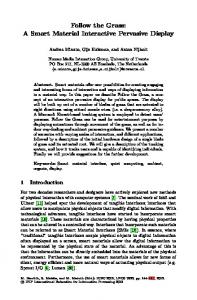
to the problem of how we can exchange Mi − O y (i) many A symbols in a front string with some of the available O y (i) − (T − (νi − 1)) A symbols in a “back string” (for a total of Mi − T + νi − 1 many A symbols) so that via a single prefix reversal we can perform transfers reflecting the structure of graph G i . This leads to the following useful definition. As a building block from which we can construct more complicated embeddings in the manner motivated above, we introduce a simple kind of co-embedding whose output is merely the length of the front string in the input string. For a graph G with no isolated vertices, we call a dilation 1 one-to-many embedding f : G → Pn a B-embedding and its associated co-embedding g a B-map if they satisfy the following conditions: (1) V (G) = {0, 1, . . . , |V (G)| − 1}. (2) Pn is defined on the symbol set A1 A2 · · · An−1 B. (3) The co-embedding g has domain R = {x ∈ V (Pn ): N x (0) < |V (G)|} and follows the simple rule g(x) = N x (0), i.e., maps each string x ∈ R to the vertex of G given by the length of the front string of x, i.e., g(A x0 BAx1 ) = x0 for all 0 ≤ x0 < |V (G)|. Figure 3 shows B-embeddings f : Q 3 → P10 and f : Q 2 → P5 . Given a graph G, since (2) and (3) entirely specify g once an assignment of vertex labels 0, 1, 2, . . . , |V (G)| − 1


417

Fig. 3. (a) A one-to-many dilation 1 embedding of Q 3 into P10 (a B-map). (b) A one-to-many dilation 1 embedding of Q 2 into P5 (a B-map).

to V (G) has been selected, it is a simple matter to decide whether G has a B-map into Pn for given n. In fact, it is easy to verify the following: for a graph G on the vertex set {0, 1, . . . , |V (G)| − 1}, there exists a B-map of G into Pn if and only if i + j < n for every edge {i, j} of G. Several observations follow quickly from this characterization: (a) If G has a minimum degree δ and a B-embedding into Pn , then n ≥ |V (G)|+δ−1 (just use i = |V (G)| − 1 above). (b) From (a), n ≥ |V (G)| for any B-map. (c) There exists a B-map for embedding the clique K m into P2m−2 , and by (a) this is optimal. (d) The hypercube embeddings in Figure 3 are optimal as B-embeddings. Before we continue, we give an important yet simple restatement of (3), as follows. For a B-map g for embedding G in Pn , where V (G) = {0, 1, . . . , |V (G)|−1} and where Pn is defined on the symbol set A1 A2 · · · An−1 B, let I denote the interval of integers I = [n − |V (G)|, n − 1]. Condition (3) is equivalent to the alternate condition that g has domain R = {x ∈ V (Pn ): N x (1) ∈ I } and follows the simple rule g(x) = n −1− N x (1), i.e., maps each string x ∈ R to the vertex of G given by the amount by which N x (1) falls short of its maximum allowable value n − 1, i.e., g(An−1−x1 BAx1 ) = n − 1 − x1 for all x1 ∈ I . This alternate rule will be used in Lemma 4 along the following general lines. We will be given B-maps gi for each of graphs G i , 1 ≤ i ≤ m. In that lemma a string x ∈ R will represent a vertex in G 1 × G 2 × G 3 · · · × G m by having each of its blocks represent a vertex of some particular factor G i . This vertex is determined by the amount by which the length of that block falls short of a specified maximum Mi . The possible such amounts will be in one-to-one correspondence with the possible values n i − 1 − x1 for the B-map gi associated with G i , and in this way will be able to toggle the i 0 th coordinate in x by closely mimicking the action of gi .

418


Lemma 4. P Let G 1 , G 2 , . . . , G m be graphs with no isolated vertices, let νi = |V (G i )|, m (νi −1). For each i suppose there exists a B-embedding f i : G i → Pni . and let T = i=1 integers, Suppose for 1 ≤ i ≤ m that Ii = [Mi−1 , Mi ] is an interval of νi many positiveP m Mi . with the largest element Mi in each Ii satisfying Mi ≥ T + n i − νi . Let M = i=1 1

Then G 1 × G 2 × G 3 × · · · × G m ⇒ Pm+M . Proof. Let Pm+M be defined on the symbol set A1 A2 · · · A M B1 B2 · · · Bm . Let G = G 1 × G 2 × · · · × G m . To go along with the B-embeddings, we assume for each i that V (G i ) = {0, 1, 2, . . . , vi − 1}, and let gi : Ri → G i be the B-map corresponding to each f i . We let R be the set of all x ∈ V (Pm+M ) for which N x (m) ∈ Im and Ox (i) ∈ Ii for each i = 1, 2, . . . , m − 1. Note that R is nonempty, since its subset A0 BA M1 BA M2 B · · · BA Mm is nonempty. Define g: R → G by the rule g(x) = (M1 − Ox (1), M2 − Ox (2), . . . , Mm−1 − Ox (m − 1), Mm − N x (m)). That is, the ith coordinate of g(x) is the amount by which the length of the block of x associated with the graph factor G i falls short of its maximum value Mi , so that the rule for g(x) is essentially derived from the various rules for the gi (see the discussion immediately preceding the lemma). We will show how to toggle any coordinate of a given y ∈ R. So let x 0 be any neighbor of g(y) = x in G, and we will show the existence of the required y 0 ∈ R, i.e., satisfying g(y 0 ) = x 0 with y 0 obtainable from y via a single prefix reversal. Let x and x 0 have their sole disagreement in the ith coordinate, with i 6= m. Also let d ≤ vi − 1 be the ith coordinate of x 0 , noting that the ith coordinate Mi − O y (i) of x is not c. Let block W j (y) have length O y (i), j < m, so that this block is the ith smallest among the first m − 1 blocks of y. From observation (b) concerning the B-map gi , we have n i ≥ vi . Since Mi ≥ T + n i − vi , we have O y (i) − (T − (vi − 1)) ≥ n i − 1 − (Mi − O y (i)) ≥ 0. Therefore W j (y) is expressible in the form A T −(vi −1) Ani −1−(Mi −O y (i)) Ar with r ≥ 0. (Here the section of T −(vi −1) many A’s are the ones available for the “even exchange” as in the discussion preceding the lemma. This leaves n i −1−(Mi − O y (i))+r , expressed as O y (i) − (T − (vi − 1)) in that same discussion, many A’s which we are free to use for adjusting the ith coordinate of g(y).) Meanwhile, W0 (y) is expressible in the form A N y (0)−(Mi −O y (i)) A Mi −O y (i) . Since gi is a B-map we are given that it is possible to exchange the A Mi −O y (i) portion of W0 (y) with exactly d of the A symbols in the Ani −1−(Mi −O y (i)) portion of W j (y) because d + (Mi − O y (i)) ≤ n i − 1 (from the property of B-maps that i + j < n for every edge ij). Observe now that N y (0) − (Mi − O y (i)) =

m−1 X

(Mk − O y (k)) + Mm − N y (m) − (Mi − O y (i))

k=1

≤

X

(vk − 1) = T − (vi − 1).

k6=i

Thus we know that the A T −(vi −1) portion of W j (y) is sufficiently large that we can perform an even exchange (as in the discussion preceding this lemma) of the entire


419

Fig. 4. How a B-embedding of each graph G i is used in constructing a dilation 1 co-embedding of G 1 × G 2 × · · · × G m into Pm+M .

A N y (0)−(Mi −O y (i)) portion of W0 (y) with N y (0) − (Mi − O y (i)) many A symbols from the A T −(vi −1) portion of W j (y). Thus block W j (y) contains sufficiently many A symbols that we can perform a prefix reversal which “reaches into” that block and does the following. It evenly exchanges N y (0) − (Mi − O y (i)) many A’s from W0 (y) with the same number of A’s from W j (y), while exchanging the remaining Mi − N y ( j) (i.e., Mi − O y (i)) many A’s reserved in W0 (y) for adjusting the ith coordinate of y with d many A’s taken from the Ani −1−(Mi −O y (i)) portion of W j (y). See Figure 4 for an illustration. Thus the resulting string y 0 has its number of A symbols in W j (y 0 ) given by N y 0 ( j) = N y ( j) + (Mi − N y ( j)) − d = Mi − d. Note that Mi − d ∈ Ii since 0 ≤ d ≤ vi − 1, fulfilling our promise that N y 0 ( j) ∈ Ii (see the discussion prior to the lemma). That is, the block W j (y) (the ith smallest among the first m − 1 blocks of y) has been transformed into the ith smallest among the first m − 1 blocks of y 0 . Therefore g(y) and g(y 0 ) agree in all but the ith coordinate. This coordinate becomes d in the resulting string y 0 obtained from y by the prefix reversal. The same argument applies when i = m, replacing each j by m and each O by N . Therefore g is a dilation 1 co-embedding. Now we reach our main result of this section, yielding reasonably efficient dilation 1 one-to-many embeddings of hypercubes and products of cliques into pancake networks. Its proof simply requires that we select appropriate choices for the numbers Mi and B-embeddings f i as in Lemma 4, verify that the hypotheses of the lemma are satisfied,

420


and compute the resulting parameters of the embedding produced by the lemma. After the proof, we say more about optimality in part (a). Theorem 4. 1

m− (a) Q n ⇒ Pk with congestion 1, where n ≥ 8 and k = 92 m 2 + 2n 2 − 4mn + 21 2 6n + 7, where m is the integer nearest (8n − 21)/18 (arbitrarily breaking any 1 n 2 + O(n) as ties for the nearest integer). Thus we have Q n ⇒ Pk , with k = 10 9 n grows. 1 (b) For the m-fold Cartesian product (K n )m of n-cliques, (K n )m ⇒ P(n−1)(3m 2 −m+2)/2 1

with congestion 1. Thus G 1 × G 2 × · · · × G m ⇒ P(n−1)(3m 2 −m+2)/2 where each G i is an arbitrary graph of order n. Proof. The claims on congestion follow immediately if we demonstrate the indicated dilation 1 embeddings, for then we use the edge routing in which P(x 0 , yx0 0 ) is just the edge x 0 − yx0 0 . We apply Lemma 4, factoring Q n as a product of lower-dimensional hypercubes. The various dimensions of the factors in this product, and the order in which these factors are listed (i.e., which factor plays the role of G i for each i in the statement of that lemma), are choices we must make. These choices help determine the dimension m + M of the pancake network into which Q n is embedded by the lemma, and we make these choices with a view to minimizing m + M. The extent to which we succeed in making the optimal choices is discussed later. In our choice of factorization, we begin by requiring each factor to be isomorphic to either Q 2 or Q 3 . Fixing the number of such factors to be m, it follows that the numbers of factors isomorphic to Q 2 and to Q 3 are 3m − n and n − 2m, respectively. Next we give a particular ordering of these factors and show how this ordering (together with the choice for the dimensions of factors above) yields, via Lemma 4, a dimension m + M equal to the expression for k given in part (a). We take the first factor to be Q 3 , each of the next 3m − n factors to be Q 2 , and each of the final n − 2m − 1 factors to be Q 3 . That is, we let G 1 = Q 3 , G i = Q 2 for each i in the interval [2, 3m − n + 1], and G i = Q 3 for each i in the interval [3m − n + 2, m]. For each factor G i isomorphic to Q 2 let f i be the B-embedding from Figure 3(b) so that n i = 5 and vi = 4 for each such i, in the notation of Lemma 4. Likewise, for each factor G i isomorphic to Q 3 let f i be the B-embedding from Figure 3(a) so that n i = 10 and vi = 8 for each such i. Therefore P T = (vi −1) = 3(3m −n)+7(n −2m) = 4n −5m. For 1 ≤ i ≤ m we can now specify the intervals Ii , where each Ii may be viewed as corresponding to the ith factor G i , by specifying the numbers Mi , 1 ≤ i ≤ m, which serve as the endpoints of these intervals. Corresponding to G 1 we let M1 = T + n 1 − v1 = 4n − 5m + 2, thereby satisfying the requirement that M1 ≥ T +n 1 −v1 . Corresponding to the next 3m −n factors isomorphic to Q 2 , we take the Mi in such a way that each interval Ii = [Mi−1 , Mi ] contains the required vi = 4 integers; that is we let Mi = M1 + 3(i − 1) = 4n − 5m − 1 + 3i for 2 ≤ i ≤ 3m − n + 1. Corresponding to the next n − 2m − 2 factors isomorphic to Q 3 we choose the Mi so that the resulting intervals [Mi−1 , Mi ], 3m − n + 2 ≤ i ≤ m − 1, contain the required vi = 8 integers; that is, we let Mi = M3n−m+1 +


421

7(i − (3m − n + 1)) = 8n − 17m − 5 + 7i for these i. Notice that all our choices for the Mi so far, that is for 1 ≤ i ≤ m − 1, satisfy Mi ≥ M1 = T + n 1 − v1 ≥ T + n i − vi , showing that the requirement Mi ≥ T + n i − vi is also satisfied. As for Mm , the lemma requires only Mm ≥ T + n m − vm = 4n − 5m + 2, so we take Mm = 4n − 5m + 2. Therefore the dimension of the pancake network into which Q n is embedded by Lemma 4 is m+M =m+

3m−n+1 X i=1

=m+

3m−n+1 X

Mi +

m−1 X

Mi + M m

i=3m−n+2

(4n − 5m − 1 + 3i) +

i=1

= 92 m 2 + 2n 2 − 4mn +

m−1 X

(8n − 17m − 5 + 7i) + Mm

i=3m−n+2 21 m 2

− 6n + 7,

giving us the expression for the dimension k claimed in part (a). Now minimizing this expression over all integers m in the relevant interval [n/3, n/2], we find by using the first derivative that the minimum occurs at the integer m so that this minimum lies in [n/3, n/2]. Substinearest (8n − 21)/18, as long as n ≥ 21 2 tuting this into the expression for k we obtain k = 10 n 2 + O(n), completing the proof 9 of (a). For part (b), in Lemma 4 use G i = K n for each of the m factors (so each vi = n and T = mn−m), and let each f i be the B-embedding from observation (c) (in the discussion immediately following the definition of B-embeddings), so that each n i = 2n − 2. Let Mm = mn − m + n − 2, and for each i < m let Mi = mn − m − 1 + i(n − 1), so that m + M = (n − 1)(3m 2 − m + 2)/2, giving the pancake network dimension as in (b). This time the intervals Ii determined are composed of vi = n many positive integers, with Mi ≥ T + n i − vi , proving (b). In devising Theorem 4(a) we used the flexibility available in factoring Q n as a product of hypercubes of smaller dimensions. The goal is naturally to find a factorization which, given n, optimizes (i.e., minimizes) the pancake dimension m + M (denoted k in the theorem) resulting from the application of Lemma 4. The factorization we used in the proof had the following features: (i) All factors are isomorphic to Q 2 or Q 3 . (ii) There are at least two factors isomorphic to Q 3 . (iii) The ordering of the factors is first Q 3 , followed by all the Q 2 factors, and finally followed by the remaining Q 3 factors. (iv) There are m = (8n − 21)/18 (rounded to the nearest integer) factors, from which it follows, using (i), that the fraction of them which are isomorphic to Q 2 and Q 3 is (3m − n)/m = 34 + o(1) and 14 + o(1), respectively. We briefly outline here a proof that this factorization is the optimum over all factorizations of Q n satisfying (i). The proof of Theorem 4(a) above already shows that among factorizations satisfying (i)–(iii), the optimum also satisfies (iv). This together with the

422


following two facts, yield the optimality of our factorization over those satisfying (i): (I) Among the factorizations satisfying (i), the optimum one also satisfies (ii). (II) Among the factorizations satisfying (i) and (ii), the optimum one also satisfies (iii). The proof of (I) comes, when n is even, from comparing the value of m + M resulting from a factorization into all Q 2 ’s with the value resulting when three of the Q 2 ’s are exchanged for two Q 3 ’s, with one of the latter placed first in the ordering of factors and the other last. The smaller value of m + M occurs with the factorization involving two Q 3 ’s. For n odd we use three Q 3 ’s in place of one Q 3 and three Q 2 ’s. The proof of (II), given a fixed number m of factors, comes in two stages. First we show that among all factorizations satisfying (i) and (ii) an optimum is attained under the ordering in which the factors G 2 , G 3 , . . . , G m−1 are arranged with all the Q 2 ’s coming first and all the Q 3 ’s coming next. This is easily seen by analyzing the effect on m + M of interchanging the order of successive factors, one of which is Q 2 and the other is Q 3 . The proof is then reduced to comparing the values of m + M resulting from the four possible orderings in which the G i , 2 ≤ i ≤ m − 1, are so arranged but where G 1 and G m can be Q 2 or Q 3 independently. A messy calculation, omitted here for brevity, shows that the optimum ordering satisfies (iii) for n ≥ 8. While we offer no proof, we believe that application of Lemma 4 using factors of dimensions other than 2 or 3 would lead to no improvement. In any case, no claim is made concerning the optimality of the embeddings behind Theorem 4(a). These embeddings are simply the best we know how to produce for large n via the restrictive but convenient sort of embedding employed in Lemma 4. 1 Note that Theorem 4(b) shows that (K 4 )n ⇒ P(9n 2 −3n+6)/2 . Thus (K 4 )n , considerably more dense than its subgraph Q 2n , is embedded into a pancake network of nearly the same dimension as the one into which Q 2n is embedded by Theorem 4(a). 3.


We next give dilation 2 embeddings of hypercubes into pancake networks. The embedding given in Theorem 5(a) is one-to-one, but is otherwise inferior to the one-to-many embedding given next in Theorem 5(b) in that the ratio of the host network dimension to the guest network dimension in the first result is considerably larger than that ratio in the second. Theorem 5. 2 (a) For n ≥ 4, Q n → P2n−2 . 2 (b) Q n ⇒ P2n , with an edge routing of congestion 4. Proof. Figure 5 shows a dilation of 2 embedding of Q 4 into P4 , proving (a) when n = 4. Straightforward iteration of Lemma 1(b) completes the proof of (a). For (b), let f 0 be the dilation 1 one-to-many embedding of Q n into DCP2n as given in Theorem 2(a). Network DCP2n embeds as a subdigraph into CP2n via the identity embedding function id, and in turn CP2n has a dilation 2 embedding f 00 into P2n , as


423

Fig. 5. A dilation 2 embedding of Q 4 into P4 .

shown in Theorem 1(a). Therefore the composition f 00 ◦ id ◦ f 0 is a one-to-many dilation 2 embedding. Concerning congestion, for any xy ∈ E(Q n ) and x 0 ∈ f (x) let yx0 0 ∈ f (y) be the designated point in f (y) at distance 2 from x 0 in P2n . The toggling corresponding to f 0 tells us that yx0 0 is obtained by performing a right cyclic shift by one symbol of some prefix of x 0 . Thus without loss of generality we can let x 0 = AqB and yx0 0 = qAB, with q a single symbol and A a length i − 1 string for some i. We define the edge routing for 2 the map Q n ⇒ P2n by letting P(x 0 , yx0 0 ) be AqB–Ar qB–qAB, a length 2 path in P2n . We refer to the edge AqB–Ar qB of P(x 0 , yx0 0 ) generated by the shorter prefix reversal as the “first” edge of P(x 0 , yx0 0 ), and to the other edge as the “second” edge of P(x 0 , yx0 0 ). Now take any edge e ∈ E(P2n ), where without loss of generality we can let e = AqB– Ar qB with A still a length i − 1 string for some i. There are two possible routing paths that could use e as a first edge, the one in the above paragraph and also Ar qB–AqB– qAr B. Now write A = α1 a1 = a2 α2 , where ai is a single symbol for i = 1, 2 and α1 (resp. α2 ) is the length i − 2 prefix (resp. suffix) of A. Then there are also two possible routing paths that could use e as a second edge, namely, α2 a2 qB–Ar qB–AqB = a2 α2 qB and α1r a1 qB–AqB–Ar qB = a1 α1r qB. Hence e is contained in at most four routing paths 2

defined for the map Q n ⇒ P2n , as required. As should be no surprise, we can do considerably better embedding into burnt pancake networks. Theorem 6.

2

Q n ⇒ BPn .

Proof. As usual let V (BPn ) be the set of all arrangements of n of the 2n burnt symbols Y1 , Y2 , . . . , Yn , Y1r , Y2r , . . . , Ynr in which exactly one symbol appears from each of the symbol pairs {Yi , Yir }. Let R = V (BPn ), and for a string S ∈ R define the co-embedding

424


g by g(S) = b1 b2 · · · bn where bi = 1 if Yi appears in reversed orientation, bi = 0 if Yi appears in ordinary orientation. To toggle the ith bit of S when burnt symbol Yi or its reverse appears as the jth symbol of S where j > 1, apply the generator rev[1, j − 1] and then rev[1, j]. This reverses the orientation of Yi without altering the orientations of any other burnt symbols. In the case j = 1 simply apply rev[1, 1]. In one instance we know of a dilation 2 embedding of an (n + 1)-dimensional hypercube into an n-dimensional burnt pancake network, an improvement over Theorem 6. This is in the case n = 2, where BP2 happens to be isomorphic to an 8-cycle, and there exists a dilation 2 embedding of Q 3 into BP2 . As we approach our next theorem it is useful to observe that the efficiency of our embeddings improves in the following sense. Prior to Theorem 6, our embeddings associated only one or a small constant number of hypercube bits per block. In Theorem 6 we succeeded in associating one hypercube bit per symbol. For the duration of the paper, we continue this trend by associating to each A symbol a bit string. In Theorem 7(b) below, each A symbol accounts for a nonconstant number k many bits of the hypercube being embedded. Hence the efficiency of our embeddings is improving as we succeed in associating progressively longer bit strings with each A symbol, in that the ratio of the dimension of the hypercube embedded to the dimension of the pancake host is increasing. This is to be expected as we allow the dilation in our embeddings to increase. Theorem 7. 2

(a) For n ≥ m, (K m )n−m+1 →, where (K m )n−m+1 = K m × K m ×· · ·× K m (n −m +1 2 factors). Thus G 1 × G 2 × · · · × G n−m+1 → CPn where each G i is an arbitrary graph of order m. 2

(b) For n ≥ 2k , Q k(n−2k +1) → CPn . Proof. Let 6k be on the symbols A1 , A2 , . . . , An−m+1 , D1 , D2 , . . . , Dm−1 . Let R be the set of those permutations of the form α0 ; D1 ; α1 ; D2 ; α2 ; D3 ; . . . ; αm−2 ; Dm−1 ; αm−1 in which within each substring αi it is the case that the A’s appear in lexicographic order, i.e., Ac appearing to the left of Ad within substring αi implies that c < d. For an arbitrary string S = α0 ; D1 ; α1 ; D2 ; . . . ; αm−2 ; Dm−1 ; αm−1 in R and an integer 1 ≤ i ≤ n−m +1 let S(i) be the index such that Ai appears within the substring α S(i) of S. Then we define the co-embedding g by g(S) = S(1); S(2); . . . ; S(n − m + 1). To toggle S(i) we can apply a single prefix cycle to bring symbol Ai to the front of the string and then another prefix cycle to move symbol Ai into any αh of our choosing, making sure that it is filed within αh lexicographically. Thus S(i) is rendered equal to any integer from 0 to m − 1 without affecting any other coordinates S( j), proving (a). Part (b) and the second part of (a) follow from the first part of (a) since G i ⊆ K m and Q k ⊆ K 2k , respectively.

4.


Continuing with the theme of using divider symbols, we present our dilation 3 result. We use the following special notation here and in the next section. Given strings


425

sm , sm+1 , . . . , sn over some alphabet, we let Con{i = m, n; si } denote the string s = sm ; sm+1 ; . . . ; sn obtained by concatenating the si in the order of increasing i proceeding along s from left to right. Theorem 8. 3

(a) (K n )k−2n ⇒ Pk , where (K n )k−2n = K n × K n × · · · × K n (k − 2n factors), with 3 k ≥ 2n. Thus G 1 × G 2 × · · · × G k−2n ⇒ Pk where each G i is an arbitrary graph of order n. (b) Let m and k be positive integers satisfying k ≥ 2 and 1 ≤ m ≤ blog2 (k)c − 1. 3

Then Q m(k−2m+1 ) ⇒ Pk . Proof. Let V (K n ) = {1, 2, . . . , n}. We view V (Pk ) as the set of permutations on the symbols B1 , B2 , . . . , Bn , D1 , D2 , . . . , Dn , A1 , A2 , . . . , Ak−2n . We define a set R ⊆ Pk and a co-embedding g: R → (K n )k−2n . For convenience, in the following description we omit the indices of the D-symbols, and just write each of them as D. We then let R be the set of all strings in Pk of the form D; α1 ; Bi1 ; α10 ; D; α2 ; Bi2 ; α20 ; D; . . . ; D; αn ; Bin ; αn0 , where the induced string α1 ; α10 ; α2 ; α20

(∗)

· · · ; αn ; αn0

is a permutation of A1 , A2 , . . . , Ak−2n . In particular, i t denotes the index of the tth B symbol from left to right. For a given S ∈ R expressed as in (∗), define g(S) as follows. For each r , 1 ≤ r ≤ k − 2n, we let β(r, S) be the index i t such that the symbol Ar is in the substring αt ; Bit ; αt0 . Thus β(r, S) indicates the subscript of the B symbol belonging to the block containing Ar . We then let g(S) = Con{r = 1, k − 2n; β(r, S)}. To see how to toggle the ith coordinate β(i, S) of string b = g(S) for a given S ∈ R, let b0 be the string obtained from b by altering the ith coordinate of b to a desired element e of V (K n ). Let e = i t and let x denote the substring αt ; Bit ; αt0 of S. We can then write S = DαDxDγ Ai δ for suitable substrings α, γ , and δ of S, where a similar argument can be given if instead x follows Ai in the string S. Now let S 0 = Dα r DAi xDγ δ, so that β(i, S 0 ) = b0 and β( j, S 0 ) = β( j, S) for any j 6= i, and hence S 0 is a string obtained from S by toggling the given bit. Finally we observe that dist(S, S 0 ) ≤ 3 via the pancake steps S → γ r Dxr Dα r DAi δ → Ai DαDxDγ δ → S 0 , thereby completing the proof of the first part of (a), the second part following since the graph product in question is a subgraph of (K n )k−2n . Part (b) then follows from the second part of (a) by letting each G i equal Q m and n = 2m . We now find a value of m which at least comes close to maximizing the hypercube dimension u(k, m) = m(k − 2m+1 ) of Theorem 8(b) for a fixed k and 1 ≤ m ≤ blog2 (k)c − 1. Letting u(m) denote u(k, m) with k fixed, we find that its derivative is u 0 (m) = k − 2m+1 (1 + m ln(2)). Observe that the equation u 0 (m) = 0 must have a unique solution since the second term on the right side of the equation for u 0 (m) is an increasing function of m. Also for large enough k we have u 0 (1) > 0 while u 0 (blog2 (k)c − 1) < 0. Hence u(m) has a unique maximum m ∗ for positive m, and this maximum does indeed occur somewhere in the interval [1, blog2 (k)c − 1] specified by Theorem 8(b).

426


Unfortunately a simple closed form solution to the equation u 0 (m) = 0 seems unavailable, so we cannot specify the maximum point m ∗ in a simple way. However, the following closer analysis pins down m ∗ within a reasonably narrow subinterval of [1, blog2 (k)c − 1]. For convenience denote log2 (k) by log(k), and let C be any constant. Now observe that if we evaluate u 0 (m) at m = log(k) − C log(log(k)) we get u 0 (log(k) − C log(log(k))) = k − 2

k (1 + ln(2)(log(k) − C log(log(k)))). [log(k)]C

It follows for any constant C > 1 that u 0 (log(k) − C log(log(k))) > 0 for large k, while for C < 1, u 0 (log(k)−C log(log(k))) < 0 for large k. Hence for any two constants α and β satisfying α < 1 < β we have log(k) − β log(log(k)) < m ∗ < log(k) − α log(log(k)) for k sufficiently large. Thus a reasonable approximation to m ∗ is log(k) − log(log(k)), leading to the choice of m used in the following corollary to Theorem 8(b). Corollary 8.1.

3

Q w(k) ⇒ Pk , where w(k) is given by

w(k) = k[log2 (k) − log2 (log2 (k))] − (2 + o(1))k. 3

Proof. By the theorem, we can obtain a map Q u(k,m ∗∗ ) ⇒ Pk , where m ∗∗ is asymptotically log2 (k) − log2 (log2 (k)), and by the discussion preceding the corollary this m ∗∗ is the near optimum choice for m in the theorem. Plugging m ∗∗ in for m in u(k, m) we get u(k, m ∗∗ ) ∼ u(k, log2 (k) − log2 (log2 (k))) · = [log2 (k) − log2 (log2 (k))] · k − 2

k log2 (k)

¸

= k[log2 (k) − log2 (log2 (k))] − (2 + o(1))k.

5.


In our next theorem giving dilation 4 embeddings, we combine the method of divider symbols with recursion. It is interesting to observe that the dimension of the hypercube we can so embed is asymptotically the same as the best known result for the dimension of the hypercube that can be embedded with dilation 4 into the star network [NSK] (see the concluding remarks). Part (i) of the theorem handles special pancake network dimensions, while part (ii) interpolates between these values. Theorem 9. 4

(i) Q (k−2)2k +2 ⇒ P2k −1 . 4

(ii) If 0 ≤ z < 2k , then Q (k−2)2k +2+z(k−1) ⇒ P2k −1+z . 4

Proof. Let T (k) = (k − 2)2k + 2. We start by showing that Q T (k) ⇒ P2k −1 . First we let the symbols of P2k −1 be B(1), B(2), . . . , B(2k−1 − 1), A(1), A(2), . . . , A(2k−1 ). Now express each string S ∈ Pn in the form S = α(0); B(i 1 ); α(1); B(i 2 );


427

α(2); . . . ; B(i m ); α(m), with m = 2k−1 − 1, where each α(i) is a string over the A’s such that the letter sets of the α(i) partition the set {A(1), A(2), . . . , A(2k−1 )}; that is, the concatenation α(1); α(2); . . . ; α(m) is a permutation of the string A(1)A(2) · · · A(2k−1 ). We proceed as usual by defining a co-embedding g: P2k −1 → Q T (k) . Let S (0) = S ∈ P2k −1 be expressed as above, and define binary strings b(r, S (0) ) of length k − 1 for each 1 ≤ r ≤ 2k−1 by letting b(r, S (0) ) be the binary equivalent of the integer i s such that A(r ) is a symbol in the substring α(s) when i s > 0, and letting it be the all 0’s string of length k − 1 when A(r ) is a symbol in the substring α(0). Thus b(r, S (0) ) indicates the subscript of the nearest B symbol to the left of A(r ). Proceeding inductively suppose that for each i, 0 ≤ i ≤ k − 2, we have constructed a string S (i) ∈ P2k−i −1 together with binary strings b(r, S (i) ) of length k − i − 1 for each 1 ≤ r ≤ 2k−i−1 . In analogy with the above, we suppose further that P2k−i −1 is defined over the symbols B (i) (1), B (i) (2), . . . , B (i) (2k−i−1 − 1), A(i) (1), A(i) (2), . . . , A(i) (2k−i−1 ), and we express each S (i) in the form S (i) = α (i) (0); B (i) (i 1 ); α (i) (1); B (i) (i 2 ); α (i) (2); . . . ; B (i) (i m ); α (i) (m), where m = 2k−i−1 − 1, and where the α (i) ’s are strings over the A(i) ’s. We call the substring B (i) (i t ); α (i) (t) of S (i) a block of S (i) with index i t , and also a block (of S) at level i (when there is no need to reference the value of the index i t ). Now let S (i+1) ∈ P2k−i−1 −1 be the string obtained from S (i) by replacing block B (i) (cd ); α (i) (d) by a symbol B (i+1) (r ) when 1 ≤ r ≤ 2k−i−2 −1 and cd = 2r , and replacing such a block by the symbol A(i+1) (r ) when 1 ≤ r ≤ 2k−i−2 and cd = 2r − 1. Thus S (i+1) can be expressed in a form similar to the one given for S (i) above, except with i replaced by i + 1 and m = 2k−i−2 − 1. We then define the length k − i − 2 binary string b(r, S (i+1) ) to be the binary equivalent of the index cd such that A(i+1) (r ) is in the block B (i+1) (cd ); α (i+1) (d) of S (i+1) . Figure 6 illustrates the inductive construction of the S (i) . Finally, we define co-embeddings gk : P2k −1 → Q T (k) by letting gk (S) = Con{i = 0, k − 2; Con{r = 1, 2k−i−1 ; b(r, S (i) )}}, that is, gk (S) is the concatenation of the various bit strings b(r, S (i) ) over all possible r and i. The cube dimension T (k) given in the codomain of gk is seen to be correct by the following induction. In base case k = 2 we have P3 defined on the letters {A(1), A(2), B(1)}. The construction associates a bit b(1, S) and b(2, S) to A(1) and A(2), respectively, this being 0 (resp. 1) if the symbol is to the left (resp. right) of B(1) in S. Hence gk (S) has length 2, in agreement with T (2) = 2. Proceeding inductively observe that there is a length k − 1 binary string associated to each of the 2k−1 many A symbols in the strings of P2k −1 . Hence level 0 contributes (k −1)2k−1 bits to gk (S) for any S ∈ P2k −1 . Assuming inductively that the codomain dimension of gk−1 is T (k −1) = (k −3)2k−1 +2, the codomain dimension of gk is therefore T (k − 1) + (k − 1)2k−1 = (k − 2)2k + 2. This completes the proof of (i). For the proof of (ii), we now consider pancakes of dimension n = 2k − 1 + z, z > 0, i.e., dimension not of the form 2k − 1. The basic idea is to pad the number of A symbols, keeping the same number of B symbols as when n = 2k − 1. We now regard Pn as being defined on the symbols {B(1), B(2), . . . , B(2k−1 −1), A(1), A(2), . . . , A(n−2k−1 +1)},

428


Fig. 6. Strings S (i) ∈ P(2k−i − 1) derived from a string S ∈ P(2k − 1).

and starting with any S ∈ Pn we form the analogous set of binary strings b(r, S (0) ), 1 ≤ r ≤ n −2k−1 +1, and b(r, S (i) ), 1 ≤ r ≤ 2k−i−1 , when i > 0. These strings describe the positions of symbols A(i) in blocks at level i, just as above. We omit the remaining nearly identical details. Though this construction applies to any integer n > 2k − 1, the dimension of the hypercube embedded in Pn is maximized when we choose k as large as possible, i.e., k = blog2 (n + 1)c. This explains the restriction on z in the statement of (ii). We now describe how to toggle any bit σ of S (as usual, σ is a bit in the string gk (S)). Let σ be contained in the substring b = b(r, S (i) ) of g(S), and let b0 be the binary string obtained from b by flipping σ . Recall that b denotes the position within S (i) of the symbol A(i) (r ) (as indicated by the index of the block at level i to which A(i) (r ) belongs). However, A(i) (r ) is in turn obtained by a sequence of coalescing operations applied to a nested sequence of substrings of S (expressed as blocks at various levels). Thus A(i) (r ) corresponds naturally to a substring x of S. Hence toggling this bit amounts to moving x to a different (and in general arbitrary) location in the string S, the latter position being determined by the string b0 . Letting S 0 be the string obtained from S in this way, we can write S as yzxt and S 0 as yxzt for suitable substrings y, z, and t. We must then show that (a) S 0 satisfies dist(S, S 0 ) ≤ 4, and (b) the strings g(S) and g(S 0 ) agree in all bits excepting σ . Statement (a) follows from the path of length 4 from S to S 0 in Pn given by yzxt → z R y R xt → x R yzt → y R x zt → yxzt. Consider now statement (b). Clearly, any two strings b(t, S (i) ) and b(t, S 0(i) ) for t 6= r are identical since no A symbol at level i other than A(i) (r ) was moved in S to obtain S 0 . So we must now compare any two strings B = b(t, S ( j) ) and B 0 = b(t, S 0( j) ) with j 6= i and t arbitrary, and show that they are identical.


429

Suppose first that j < i. Now B is the index of the block in S ( j) containing A( j) (t), and this block remains a single symbol or is coalesced into other symbols at higher levels. It follows that A( j) (t) is contained in this block under any movements of symbols at the higher level i required to obtain S 0 . Hence B and B 0 are identical. Now suppose that j > i. Thinking of B as the block index of the substring x of S corresponding to A( j) (t), we see that movements of A symbols at lower levels (resulting in S 0 ) possibly change the composition of x but do not change the index. Hence B and B 0 are identical. Thus (b) is proved. We now determine the cube dimension associated with the embedding for arbitrary n = 2k − 1 + z. Observe that the co-embedding g associates a length k − 1 bit string with each of the A symbols (at level 0) used to increase the number of A symbols (that number now being n − 2k−1 + 1). The rest of the construction is identical, so now the cube dimension is (k − 2)2k + 2 + z(k − 1), as required.

6.

Concluding Remarks

The focus of this paper has been the construction of very low dilation maps of hypercubes into pancake (or related substring reversal) networks as a step in the simulation of the former by the latter. A subsidiary goal has been to show how the technique of one-to-many embeddings can be useful in such constructions. For a fixed pancake network, there is a tradeoff between the size of the hypercube embedded and the dilation for such maps. We therefore list below the largest dimension d (as a function of n) for which we have succeeded in embedding Q d into Pn , indicating the relevant result. The notation 2( f (n)) stands as usual for a function whose absolute value is bounded above and below by a constant multiple of f (n) for n large. The usefulness of the one-to-many embedding technique is clear from our ability to embed a hypercube of higher dimension in Pn than we are able to via a one-to-one embedding at D

these low dilations. For D = 1 we obtained embeddings Q d → SSRn , where d = 2(n), from Theorem 3(c). While this shows that for dilation 1 we were able to embed a larger hypercube into SSRn than into Pn , this is no surprise because of the higher degree 2(n 2 ) in SSRn compared with 2(n) in Pn . Largest dimension d for which our Dilation D 1 2

D

constructions give Q d ⇒ Pn √ 3 √ n + O(1) (congestion 1) 10

1 2 n,

for n even

(congestion 4)

3

n(log(n) − log(log(n))) − (2 + o(1))n

4

n log(n) − (2 + o(1))n

Reference Theorem 4 Theorem 5 Corollary 8.1 Theorem 9

The threshold dilation D = 4 seems like a natural place to stop when investigating very low dilation maps of hypercubes into pancake networks. First, the dimension d = n log(n) − (2 + o(1))n of the embedded hypercube matches that obtained (implicitly)

430


in [NSK] for one-to-one and dilation at most 4 embeddings Q d → Sn of a hypercube into the star network Sn of dimension n. The latter is the Cayley graph G(6n , Tn ) on 6n with a generator set Tn consisting of the n − 1 transpositions through the first position, that is, Tn = {(1, i): 2 ≤ i ≤ n}. Extending the result of [NSK], maps Q d → Sn and Q d → Pn were constructed [MPS2] with the larger hypercube dimension d = n log(n) − ( 32 + o(1))n and dilation bounded above by a constant K , but where K is considerably larger than 4. Thus dilation 4 seems a natural “largest” very low dilation to investigate in this context. Of course, the interesting problem remains of investigating D how large d can be in a map Q d → Pn or Q d ⇒ Pn with reasonably small dilation (say bounded by some constant or slowly growing function of n), and what tradeoff exists between dilation D and hypercube dimension d in such a map. We conclude with the reference table below of the substring reversal networks studied in this paper: Network

Vertices

Edges AB

Pn

all n! strings of length n obtained by permuting the symbols {1, 2, . . . , n}

B is obtained from A by reversing any initial substring of A; that is, A = S; T and B = S r ; T for suitable S and T

BPn

all 2n n! strings of length n over the alphabet {1, 2, . . . , n, 1r , 2r , . . . , n r }, where for each i exactly one of {i, i r } appears in the string

r A = x1 x2 · · · xn , B = xir xi−1 · · · x1r xi+1 xi+2 · · · xn for some i, where if xt = m r for some m, then xtr = m

SSRn

The same as for Pn

B is obtained from A by reversing any substring of A; that is, A = R; S; T and B = R; S r ; T for substrings R, S, T with |S| ≥ 2, with R or T possibly empty

BSSRn

The same as for BPn

B is obtained from A by reversing any substring of A, and in the process reversing each symbol in the reversed substring; that is, A = x1 x2 r · · · xn and B = x1 x2 · · · xi−1 x jr x j−1 · · · xir x j+1 x j+2 · · · xn for some i and j. Again if xt = m r , then xtr = m

CPn

The same as for Pn

B is obtained from A by a cyclic rotation, in either direction, of an initial substring of A; that is, A = q; S; R and B = S; q; R, or A = S; q; R and B = q; S; R, where q is a single symbol

DCPn (directed)

The same as for Pn

B is obtained from A by a right cyclic shift of an initial substring of A; that is, A = S; q; R and B = q; S; R, where q is a single symbol. Thus AB is a directed edge from A to B

References [AK]

S. Akers and B. Krishnamurthy, A group-theoretic model for symmetric interconnection networks, IEEE Trans. Comput., 38(4) (1989), 555–566. [AKM] S. G. Akl, Q. Ke, and H. Meyer, On some properties and algorithms for the star and pancake interconnection networks, J. Parallel Distrib. Comput., 22(1) (1994), 16–25.

One-to-Many Embeddings of Hypercubes into Cayley Graphs Generated by Reversals [AQS] [BCH+ ] [BCLR] [BFP]

[BHOS]

[BMPS]

[C] [CB]

[F] [FMC] [GP] [GVV] [HS]

[K] [KLM+ ] [L] [LMR] [M1] [M2] [MPS1] [MPS2] [MS1] [MS2]

[MW] [NSK]

431

S. G. Akl, K. Qiu, and I. Stojmenovic, Fundamental algorithms for star and pancake interconnection networks with application to computational geometry, Networks, 23(4) (1993), 215–225. S. N. Bhatt, F. R. K. Chung, J. W. Hong, F. T. Leighton, and A. L. Rosenberg, Optimal simulations by butterfly-like networks, J. Assoc. Comput. Mach., 43(2) (1996), 293–330. S. N. Bhatt, F. R. K. Chung, F. T. Leighton, and A. L. Rosenberg, Efficient embeddings of trees in hypercubes, SIAM J. Comput. (1992), 151–162. P. Berthome, A. Ferreira, and S. Perennes, Optimal information dissemination in star and pancake networks, in Proc. 1993 Fifth IEEE Symp. on Parallel and Distributed Processing, IEEE Computer Society Press, Los Alamitos, CA, 1995. A. Bouabdallah, M. C. Heydemann, J. Opatrny, and D. Sotteau, Embedding complete binary trees into star and pancake graphs, Manuscript, Computer Science Department, Concordia University, Montreal, 1993. S. Bettayeb, Z. Miller, T. Peng, and I. H. Sudborough, Embedding d-D meshes into optimum hypercubes with dilation 2d − 1, in Parallel and Distributed Computing—Theory and Practice (First Canada– France Conf. Proc.) (Cosnard, Ferreira, Peters, eds.), Lecture Notes in Computer Science, vol. 805, Springer-Verlag, Berlin, 1994, pp. 73–80. M. Y. Chan, Embedding of grids into optimal hypercubes, SIAM J. Comput. (1991), 834–864. D. S. Cohen and M. Blum, Improved bounds for sorting pancakes under a conjecture, to appear in Algorithms. Available from Computer Science Division, University of California, Berkeley, CA, May 1992. M. Fellows, Encoding graphs in graphs, Ph.D. Dissertation, Department of Computer Science, University of California, San Diego, CA, 1985. V. Faber, J. W. Moore, and W. Y. C. Chen, Cycle prefix digraphs for symmetric interconnection networks, Networks, 23 (1993), 641–649. W. H. Gates and C. H. Papadimitriou, Bounds for sorting by prefix reversal, Discrete Math, 27 (1979), 47–57. L. Gargano, U. Vaccaro, and A. Vozella, Fault tolerant routing in the star and pancake interconnection networks, Inform. Process. Lett., 45(6) (1993), 315–320. M. H. Heydari and I. H. Sudborough, On sorting by prefix reversals and the diameter of pancake networks, in Proc. First Heinz Nixdorf Symp., November 1992, Lecture Notes in Computer Science, vol. 678, Springer-Verlag, Berlin, 1993, pp. 218–227. A. Kanevsky, On the embedding of cycles in pancake graphs, Parallel Comput., 21(6) (1995), 923–936. R. Koch, F. T. Leighton, B. M. Maggs, S. B. Rao, A. L. Rosenberg, and E. J. Schwabe, Work preserving emulations of fixed-connection networks, J. Assoc. Comput. Mach., 44(1) (1997), 104–147. F. T. Leighton, Introduction to Parallel Algorithms and Architectures: Arrays, Trees, Hypercubes, Morgan Kaufmann, San Mateo, CA, 1992. F. T. Leighton, B. Maggs, and S. Rao, Universal packet routing algorithms, in Proc. 29th Annual Symp. on Foundations of Computer Science, IEEE, New York, 1988, pp. 256–271. F. Meyer Auf Der Heide, Efficiency of universal parallel computers, Acta Inform., 19 (1983), 269–296. F. Meyer Auf Der Heide, Efficient simulations among several models of parallel computers, SIAM J. Comput., 19 (1986), 106–119. Z. Miller, D. Pritikin, and I. H. Sudborough, Near embeddings of hypercubes into Cayley graphs on the symmetric group, IEEE Trans. Comput., 43(1) (1994), 13–22. Z. Miller, D. Pritikin, and I. H. Sudborough, Bounded dilation maps of hypercubes into Cayley graphs on the symmetric group, Math. Systems Theory, 29 (1996), 551–572. B. Monien and I. H. Sudborough, Embedding one interconnection network into another, Computing (Computing Suppl. 7), Springer-Verlag, New York, 1990, pp. 257–282. B. Monien and I. H. Sudborough, Simulating binary trees on hypercubes, in Proc. 1988 AWOC Conf. on VLSI Algorithms and Architectures (July 1988), Lecture Notes in Computer Science, vol. 319, Springer-Verlag, Berlin, 1994, pp. 170–180. F. Meyer Auf Der Heide and R. Wanka, Time-optimal simulations of networks by universal parallel computers, in Proc. 6th Symp. on Theoretical Aspects of Computer Science, 1989, pp. 120–131. M. Nigam, S. Sahni, and B. Krishnamurthy, Embedding hamiltonians and hypercubes in star interconnection graphs, in Proc. Internat. Conf. on Parallel Processing, vol. III, 1990, pp. 340–343.

Received July 30, 1997, and in revised form July 18, 2001. Online publication October 30, 2001.

Theory of Computing Systems - Springer Link

Theory of Computing Systems - Springer Link

Suggest Documents

Theory of Computing Systems - Springer Link

Theory of Computing Systems - People

Theory of Computing Systems - CiteSeerX

Theory of Computing Systems - CiteSeerX

Theory of Computing Systems - CiteSeerX

Theory of Computing Systems - CiteSeerX

Theory of Computing Systems - People

Theory of Computing Systems - LaBRI

Theory of Computing Systems - Lirmm

Theory of Computing Systems - CiteSeerX

Theory of Computing Systems - CiteSeerX

systems and systems theory, clusters and networks - Springer Link

Sentic Computing - Springer Link

Computing Integrals - Springer Link

Computing Compliance - Springer Link

Entertainment Computing - Springer Link

Creative destruction of computing systems: analysis ... - Springer Link

Theory of Computing Systems - Research - MIT

Design Theory - Springer Link

Field Theory - Springer Link

Advances in Intelligent Systems and Computing - Springer Link

Advances in Intelligent Systems and Computing - Springer Link

Advances in Intelligent Systems and Computing - Springer Link