My stay at Caltech has been a very fruitful, rewarding and enjoyable ... tech) on different projects over the years, some of which will continue even after I.
Theory of electronically nonadiabatic quantum reaction dynamics
Thesis by
Ravinder Abrol
In Partial Fulfillment of the Requirements for the Degree of Doctor of Philosophy
California Institute of Technology Pasadena, California
2003 (Defended 26 November 2002)
ii
c 2003
Ravinder Abrol All Rights Reserved
iii
Dedicated to my parents... ...for their boundless support and patience
iv
Acknowledgements My stay at Caltech has been a very fruitful, rewarding and enjoyable experience that I will cherish forever. This experience was made possible by the presence of a great set of people around me, who never let me feel that I was living so far away from my family. First and foremost, I would like to acknowledge the constant support and encouragement of my research adviser Professor Aron Kuppermann, who along with Roza treated me like family and took very good care of me. Interaction with Aron has not only helped me in my professional development, but also strengthened my belief in a satisfying scientific pursuit. At every stage of this work, he provided full intellectual freedom without making me loose sight of the big picture and made sure that all resources were available whenever needed. I thank him for being an excellent adviser and am already looking forward to working with him after I leave this place. My thesis committee members (besides Aron) Prof. Vince McKoy, Prof. Harry Gray and Prof. Rudy Marcus along with Prof. Mitchio Okumura have been excellent mentors and provided a lot of encouragement over the years. The time I spent in the lab was made enjoyable by: Desheng Wang, who was always available for serious scientific discussions or just casual chat; Stephanie Rogers, who helped me when I joined the group and over the years; and finally Mark Wu and Ken Museth, both of whom helped me with many problems. Sharon Brunett from Center of Advanced Computing Research provided precious help with porting of our scattering code to MPI message passing system. It has been a pleasure to collaborate with Prof. David Yarkony (Johns Hopkins University), Prof. Laurent Wiesenfeld (University of Grenoble, France), Dr. Vidyasankar Sundaresan (The Scripps Research Institute), Dr. Rick Muller (Caltech) and Bruce Lambert (Caltech) on different projects over the years, some of which will continue even after I leave Caltech. The work in this thesis has been supported in part by NSF Grants
v CHE-9810050 and CHE-0138091. I would also like to thank Dr. Prashant Purohit (Caltech) for suggesting the derivation given in Appendix 4.A of Chapter 4 of this thesis. Ms. Billie Tone has been a lot of fun to work and chat with over the years. Weitekamp group and Zewail group members have been great neighbours. Prof. N. Sathyamurthy (Indian Institute of Technology, Kanpur, India) has provided a lot of encouragement to my scientific ambitions. Outside the lab, my experience has been made truely memorable by Tara, Sandeep, Vidya, Kirana, Goutam, Sulekha, Nitin, Amit, Ramesh, Shachi, MA, Suresh, Supraja, Ganesh, Anu, Jeetu, Nandita, Prakash, Swami, Ashish, Anu, Harish, Anitha, Sujata, Neha, Tejaswi, Pratip, Rajesh, Arjun, Prashant, Abhijit, Parandeh, Victoria, Dela, David, Hans Michael, Hsing, Stephanie Chow, Michael van Dam, Michael Fleming, Jim Kempf, Roni, Shervin, Office of International Student Programs and others. The cricket games, red-door coffee breaks, potlucks, international orientation, soccer games with the Chemistry team Kicking Buck and OASIS programs were times very well spent. My other friends in India/USA, who include Sushant, Sachchidanand, Anju, Suman, Sangeeta, Rajiv, Anjali, Monika, Aditya, Deepak, Manoj, Anand, Saurabh, Vishy, Kaustav, Neelanjana, Jonaki, Shankarshan and a few others provided great times chatting over the phone or in person whenever we met. Chhavi and her family never let me feel that I was living so far away from home and took very good care of me. She has provided tremendous support and encouragement every step of the way. The journey to the completion of this thesis would have been much harder without her. Finally, my extended family back home receives all the kudos for their patience and constant encouragement over the years. My Shibu Mama and Sushma Mami have provided a rock solid foundation and support to me without which I wouldn’t be here. My parents have taught me honesty and diligence and encouraged me to pursue anything that makes me happy. Their love and support has made me believe in myself and I dedicate this thesis to them and their life-long hard work.
vi
Abstract In most quantum descriptions of chemical reactions, the Born-Oppenheimer (BO) approximation is invoked that separates the motion of light electrons and heavy nuclei, thereby restricting the motion of those nuclei to a single adiabatic electronic state. Intersections between neighboring electronic states are more common in molecular systems of interest to chemistry and biology than in diatomic molecules. The picture is further complicated due to nonadiabatic couplings which can be present in these systems even in the absence of intersections between electronic states. These couplings are solely responsible for all nonadiabatic effects in chemical and biological processes. For understanding these nonadiabatic effects, the BO picture needs to be replaced by the general Born-Huang (BH) description, in which the nuclei can sample an arbitrary number of electronic states. A general BH treatment is presented for a polyatomic system evolving on n adiabatic electronic states. All nonadiabatic couplings are considered in this adiabatic representation. These couplings can be singular for electronically degenerate nuclear geometries. The presence of these nonadiabatic couplings (even if not singular) can lead to numerical inefficiencies in the solution of the corresponding nuclear motion Schr¨odinger equation. This problem is circumvented by going to a diabatic representation, in which these couplings are not only never singular but are also minimized over the entire dynamically important nuclear configuration space. This BH description is applied to the benchmark triatomic system H3 by obtaining an optimal diabatic representation of its lowest two adiabatic electronic states. A two-electronic-state quantum dynamics formulation is also presented, which, in addition to providing reaction cross sections over a broad energy range, will also enable a quantitative test of the validity of the BO approximation.
vii
Contents Acknowledgements
iv
Abstract
vi
1 Introduction 2 Born-Huang treatment of an N -body system
1 11
2.1
Introduction . . . . . . . . . . . . . . . . . . . . . . . . . . . . . . . .
11
2.2
Born-Huang expansion . . . . . . . . . . . . . . . . . . . . . . . . . .
14
2.2.1
Adiabatic nuclear motion Schr¨odinger equation . . . . . . . .
15
2.2.2
First-derivative coupling matrix . . . . . . . . . . . . . . . . .
15
2.2.3
Second-derivative coupling matrix . . . . . . . . . . . . . . . .
17
Adiabatic-to-diabatic transformation . . . . . . . . . . . . . . . . . .
18
2.3.1
Electronically diabatic representation . . . . . . . . . . . . . .
18
2.3.2
Diabatic nuclear motion Schr¨odinger equation . . . . . . . . .
20
2.3.3
Diabatization matrix . . . . . . . . . . . . . . . . . . . . . . .
22
2.3
3 Accurate first-derivative nonadiabatic couplings for H3 system
32
3.1
Introduction . . . . . . . . . . . . . . . . . . . . . . . . . . . . . . . .
32
3.2
Theory and numerical methods . . . . . . . . . . . . . . . . . . . . .
37
3.2.1
Ab initio couplings and electronic energies . . . . . . . . . . .
37
3.2.2
DMBE couplings and electronic energies . . . . . . . . . . . .
41
viii 3.3
3.4
Ab initio and DMBE electronic energies . . . . . . . . . . . . . . . .
42
3.3.1
Fitting method . . . . . . . . . . . . . . . . . . . . . . . . . .
42
3.3.2
DSP and DMBE potential energy surfaces . . . . . . . . . . .
44
Results and discussion . . . . . . . . . . . . . . . . . . . . . . . . . .
48
3.4.1
Ab initio and DMBE first-derivative couplings . . . . . . . . .
48
3.4.2
The topological phase
. . . . . . . . . . . . . . . . . . . . . .
51
3.4.3
Discussion . . . . . . . . . . . . . . . . . . . . . . . . . . . . .
52
4 An optimal diabatization of the lowest two states of H3
87
4.1
Introduction . . . . . . . . . . . . . . . . . . . . . . . . . . . . . . . .
87
4.2
Methodology . . . . . . . . . . . . . . . . . . . . . . . . . . . . . . .
94
4.2.1
Coordinate system . . . . . . . . . . . . . . . . . . . . . . . .
94
4.2.2
The Poisson equation . . . . . . . . . . . . . . . . . . . . . . .
95
4.2.3
Boundary conditions for solving the Poisson equation . . . . .
96
4.2.4
Numerical solution of the Poisson equation . . . . . . . . . . .
98
4.3
Results and discussion . . . . . . . . . . . . . . . . . . . . . . . . . . 106 4.3.1
Diabatization angle . . . . . . . . . . . . . . . . . . . . . . . . 106
4.3.2
Longitudinal and transverse parts of the first-derivative coupling vector . . . . . . . . . . . . . . . . . . . . . . . . . . . . 109
4.3.3
Diabatic potential energy surfaces . . . . . . . . . . . . . . . . 111
4.3.4
Discussion . . . . . . . . . . . . . . . . . . . . . . . . . . . . . 113
5 A two-electronic-state nonadiabatic quantum scattering formalism 156 5.1
Introduction . . . . . . . . . . . . . . . . . . . . . . . . . . . . . . . . 156
5.2
Symmetrized hyperspherical coordinates . . . . . . . . . . . . . . . . 159
ix 5.3
5.4
Adiabatic formalism . . . . . . . . . . . . . . . . . . . . . . . . . . . 164 5.3.1
Partial wave expansion . . . . . . . . . . . . . . . . . . . . . . 167
5.3.2
Propagation scheme and asymptotic analysis . . . . . . . . . . 178
Diabatic formalism . . . . . . . . . . . . . . . . . . . . . . . . . . . . 180 5.4.1
Partial wave expansion . . . . . . . . . . . . . . . . . . . . . . 183
5.4.2
Propagation scheme and asymptotic analysis . . . . . . . . . . 188
5.4.3
Adiabatic vs. diabatic approaches . . . . . . . . . . . . . . . . 189
6 Summary and conclusions
203
1
Chapter 1
Introduction
Electronic transitions (excitations or deexcitations) can take place during the course of a chemical reaction and have important consequences for its dynamics. The motions of electrons and nuclei were first analyzed in a quantum-mechanical framework by Born and Oppenheimer [1], who separated the motion of the light electrons from that of the heavy nuclei and assumed that the nuclei moved on a single adiabatic electronic state or potential energy surface (PES). This Born-Oppenheimer (BO) approximation can break down due to the presence of strong nonadiabatic couplings between degenerate electronic states (due to conical, parabolic or glancing intersections between those states) or between the near-degenerate ones (due to avoided crossings). These couplings allow for the motion of nuclei on coupled multiple adiabatic electronic states, with the BO approximation replaced by the Born-Huang expansion [2, 3] in which an arbitrary number of electronic states can be included. A recent volume of Advances in Chemical Physics [4] deals with understanding the issues surrounding the role played by degenerate electronic states in determining the mechanism and outcome of many chemical processes. These nonadiabatic couplings that give rise to electronic transtions can be classified into two categories: (a) Radial couplings, which have been treated by Zener [5], Landau [6] and others [7–12], arise due to translational, vibrational and angular motions of the atomic or molecular species involved in the chemical process. These couplings allow for transitions to occur between electronic states of the same symmetry. (b) Rotational couplings, which have been studied by Kronig [13] and others [14–20], arise as a result of a transformation of molecular coordinates from a space-fixed (SF) frame to a body-fixed (BF) one due to the conservation of total electron plus nuclear angular momentum. These couplings allow for transitions between electronic states of the same as well as of different symmetries.
2 An important consequence of the presence of degenerate electronic states is the geometric phase effect. For a polyatomic system involving N atoms, where N ≥ 3, any two adjacent adiabatic electronic states can be degenerate for a set of nuclear geometries even if those electronic states have the same symmetry and spin multiplicity [21]. These intersections occur more frequently in such polyatomic systems than in the diatomic world. The reason is that these systems possess three or more internal nuclear motion degrees of freedom, and only two independent relations between three electronic Hamiltonian matrix elements (in a simple two-electronic-state picture) are sufficient for the existence of doubly degenerate electronic energy eigenvalues. As a result, these relations can easily be satisfied explaining thereby the frequent occurrence of intersections. If the lowest order terms in the expansion of these elements in displacements away from the intersection geometry are linear (as is usually the case), these intersections are conical, the most common type of intersection. Assuming the adiabatic electronic wave functions of the two intersecting states to be real and as continuous as possible in nuclear coordinate space, if the polyatomic system is transported along a closed loop in that space (a so-called pseudorotation) that encircles one conical intersection geometry, these electronic wave functions must change sign [21, 22]. This change of sign requires the adiabatic nuclear wave functions to undergo a compensatory change of sign, known as the geometric phase (GP) effect [23–27], to keep the total wave function single-valued. This sign change of the nuclear wave function, which is a special case of Berry’s geometric phase [26], is also referred to as the molecular Aharonov-Bohm effect [28] and has important consequences for the structure and dynamics of the polyatomic system being considered, as it greatly affects the nature of the solutions of the corresponding nuclear motion Schr¨odinger equation [27]. The dynamics of chemical reactions on a single ground adiabatic electronic PES has been studied extensively over the last few decades using accurate quantummechanical time-dependent and time-independent methods. These studies have been successfully applied to triatomic [29–31] and tetraatomic [32–34] reactions in the ab-
3 sence of conical intersections. In the last decade or so, these studies have included indirectly the effect of the first-excited adiabatic electronic state, that intersects conically with the ground state, by introducing the GP effect through appropriate boundary conditions on the adiabatic nuclear wave function corresponding to the ground electronic state [35–41]. The reaction rates (products of initial relative velocities by integral cross sections) for the D + H2 reaction, obtained with the GP effect included [37], were in much better agreement with the experimental results [42–45] than those obtained with the GP effect excluded. Although the GP effect is certainly more pronounced at resonance energies [46], its importance for differential cross sections has been the topic of hot debate recently [40, 41]. Many studies have appeared in the last few years that include two or more excited electronic states and nonadiabatic couplings between them to study nonadiabatic behavior in chemical reactions. The effect of spin-orbit couplings on electronically nonadiabatic transitions has been demonstrated for many chemical systems [47–56]. The photodissociation of triatomic molecules like O3 and H2 S has been studied on their conically intersecting potential energy surfaces (PESs) [57, 58]. The benchmark H + H2 reaction has also been studied on its lowest two conically intersecting PESs, but only for total angular momentum quantum number J = 0 [59]. Most of these studies have been made possible due to the availability of realistic ab initio electronic PESs and their nonadiabatic couplings [60]. These nonadiabatic couplings have very interesting properties that have a forebearing on the behavior of molecular systems and are currently the topic of active interest [61]. The singular nature of these couplings at the conical intersections of two adiabatic electronic states introduces numerical difficulties in the solution of the corresponding coupled adiabatic nuclear motion Schr¨odinger equations. These difficulties can be circumvented by transforming the electronically adiabatic representation into a quasi-diabatic one [62–74], in which the nonadiabatic couplings still appear but are not singular. In this thesis, a rigorous quantum-mechanical formalism is introduced for studying the dynamics of a polyatomic system (comprising of N atoms) on n electronically
4 adiabatic states, interacting due to the presence of nonadiabatic couplings. The spin-spin and spin-orbit interactions are not considered. These interactions can be introduced subsequently as perturbative corrections, if they are not too large. This formalism is then applied to a triatomic system in a two-electronic-state Born-Huang approximation. The overview of the thesis is as follows. In Chapter 2, the adiabatic n-electronic-state coupled nuclear motion Schr¨odinger equations are presented for an N -body system and the properties of first-derivative and second-derivative nonadiabatic couplings are discussed. The presence of firstderivative couplings, that may be singular at electonically degenerate nuclear configurations, can lead to numerical inefficiencies in the solution of the adiabatic Schr¨odinger equations.
A diabatic representation is defined through an adiabatic-to-diabatic
transformation that minimizes the magnitude of the first-derivative nonadiabatic couplings in the diabatic nuclear motion Schr¨odinger equations. This formalism is applied in Chapters 3 through 5 to a triatomic system in the presence of two interacting electronic states. In Chapter 3, accurate first-derivative nonadiabatic coupling vectors are presented for H3 system that exhibits a conical intersection between its ground (1 2 A0 ) and its first-excited (2 2 A0 ) electronic states. These coupling vectors, which are singular at the conical intersection geometries, and the two electronic states they couple are fitted using their ab initio data and compared with their approximate analytical counterparts obtained by Varandas et al. [75] using the double many-body expansion (DMBE) method. Contour integrals of the ab initio first-derivative couplings, calculated along closed loops around the abovementioned conical intersection, contain important properties of these couplings besides information about possible interactions between the 2 2 A0 and the second-excited (3 2 A0 ) states. The second-derivative couplings are approximated by using the abovementioned accurate first-derivative coupling vectors in a two-electronic-state model. These coupling vectors between the corresponding electronically adiabatic states can be decomposed into longitudinal (removable) and transverse (nonremovable)
5 parts. This property is used in Chapter 4 to obtain a diabatic representation for the lowest two adiabatic electronic states of H3 , in which singular nonadiabatic couplings are replaced by non-singular ones. The adiabatic-to-diabatic transformation is achieved by solving a three-dimensional Poisson equation over the entire internal nuclear configuration space. The boundary conditions imposed on this solution minimize the magnitude of the nonremovable couplings that survive in the diabatic representation. This makes the diabatic language a convenient one for studying quantum reactive scattering on more than one interacting electronic states. In Chapter 5, an electronically nonadiabatic reactive scattering formalism is presented for triatomic reactions involving two coupled adiabatic electronic states in adiabatic and diabatic languages. This formalism is an extension of the time-independent coupled-channel hyperspherical coordinate method [18] used in the past to study such reactions on a single adiabatic Born-Oppenheimer (BO) electronic state. Both adiabatic and diabatic representations lead to a set of coupled nuclear motion Schr¨odinger equations that can be solved to obtain scattering matrices, which then furnish the differential and integral cross sections. The advantages and disadvantages of the two languages are discussed. This formalism will not only provide reaction cross sections over a broad energy range (including those energies where the BO approximation breaks down), but will also enable a comparison with the cross sections obtained using only the ground adiabatic PES (with the geometric phase included), to estimate the validity of the one-electronic-state BO approximation as a function of energy.
6
Bibliography [1] M. Born and J. R. Oppenheimer, Ann. Phys. (Leipzig) 84, 457 (1927). [2] M. Born, Nachr. Akad. Wiss. G¨ott. Math.-Phys. Kl. Article No. 6, 1 (1951). [3] M. Born and K. Huang, Dynamical Theory of Crystal Lattices (Oxford University Press, Oxford, 1954), pp. 166-177 and 402-407. [4] The Role of Degenerate States in Chemistry: A Special Volume of Advances in Chemical Physics, eds. M. Baer and G. D. Billing (Wiley-Interscience, New York, 2002), Vol. 124. [5] C. Zener, Proc. R. Soc. London Ser. A 137, 696 (1932). [6] L. D. Landau, Phys. Z. Sowjetunion 2, 46 (1932). [7] E. C. G. Stuckelberg, Helv. Phys. Acta. 5, 369 (1932). [8] N. Rosen and C. Zener, Phys. Rev. 40, 502 (1932). [9] W. Lichten, Phys. Rev. 131, 229 (1963). [10] E. E. Nikitin, in Chemische Elementarprozesse, edited by H. Hartmann (Springer-Verlag, Berlin, 1968), 43. [11] F. T. Smith, Phys. Rev. 179, 111 (1969). [12] M. S. Child, Mol. Phys. 20, 171 (1971). [13] R. de L Kronig, Band Spectra and Molecular Structure, Cambridge University Press, New York, 1930, 6. [14] D. R. Bates, Proc. R. Soc. London Ser. A 240, 437 (1957).
7 [15] D. R. Bates, Proc. R. Soc. London Ser. A 257, 22 (1960). [16] W. R. Thorson, J. Chem. Phys. 34, 1744 (1961). [17] D. J. Kouri and C. F. Curtiss, J. Chem. Phys. 44, 2120 (1966). [18] R. T. Pack and J. O. Hirschfelder, J. Chem. Phys. 49, 4009 (1968). [19] C. Gaussorgues, C. Le Sech, F. Mosnow-Seeuws, R. McCarroll and A. Riera, J. Phys. B 8, 239 (1975). [20] C. Gaussorgues, C. Le Sech, F. Mosnow-Seeuws, R. McCarroll and A. Riera, J. Phys. B 8 253 (1975). [21] G. Herzberg and H. C. Longuet-Higgins, Discussion Faraday Soc. 35, 77 (1963). [22] H. C. Longuet-Higgins, Proc. R. Soc. London A 344, 147 (1975). [23] H. C. Longuet-Higgins, Adv. Spectrosc. 2, 429 (1961). [24] C. A. Mead and D. G. Truhlar, J. Chem. Phys. 70, 2284 (1979). [25] C. A. Mead, Chem. Phys. 49, 23 (1980). [26] M. V. Berry, Proc. Roy. Soc. London, Ser. A 392, 45 (1984). [27] A. Kuppermann, in Dynamics of Molecules and Chemical Reactions, edited by R. E. Wyatt and J. Z. H. Zhang (Marcel Dekker, New York, 1996), pp. 411-472. [28] Y. Aharonov and D. Bohm, Phys. Rev. 115, 485 (1969). [29] Theory of Chemical Reaction Dynamics Vols. I and II, edited by M. Baer (CRC Press, Boca Raton (Florida), 1985). [30] Dynamics of Molecules and Chemical Reactions, edited by R. E. Wyatt and J. Z. H. Zhang (Marcel Dekker, New York, 1996). [31] G. Nyman and H.-G. Yu, Rep. Prog. Phys. 63, 1001 (2000).
8 [32] J. Z. H. Zhang, J. Q. Dai, and W. Zhu, J. Phys. Chem. A 101, 2746 (1997). [33] S. K. Pogrebnya, J. Palma, D. C. Clary, and J. Echave, Phys. Chem. Chem. Phys. 2, 693 (2000). [34] D. H. Zhang, M. A. Collins and S. Y. Lee, Science 290, 961 (2000). [35] Y.-S. M. Wu, A. Kuppermann, and B. Lepetit, Chem. Phys. Lett. 186, 319 (1991). [36] Y.-S. M. Wu and A. Kuppermann, Chem. Phys. Lett. 201, 178 (1993). [37] A. Kuppermann and Y.-S. M. Wu, Chem. Phys. Lett. 205, 577 (1993). [38] Y.-S. M. Wu and A. Kuppermann, Chem. Phys. Lett. 235, 105 (1995). [39] A. Kuppermann and Y.-S. M. Wu, Chem. Phys. Lett. 241, 229 (1995). [40] B. K. Kendrick, J. Chem. Phys. 112, 5679 (2000); 114, 4335 (2001) (E). [41] A. Kuppermann and Y.-S. M. Wu, Chem. Phys. Lett. 349, 537 (2001). [42] D. A. V. Kliner, K. D. Rinen, and R. N. Zare, Chem. Phys. Lett. 166, 107 (1990). [43] D. A. V. Kliner, D. E. Adelman and R. N. Zare, J. Chem. Phys. 95, 1648 (1991). [44] D. Neuhauser, R. S. Judson, D. J. Kouri, D. E. Adelman, N. E. Shafer, D. A. V. Kliner and R. N. Zare, Science 257, 519 (1992). [45] D. E. Adelman, N. E. Shafer, D. A. V. Kliner and R. N. Zare, J. Chem. Phys. 97, 7323 (1992). [46] F. Fernandez-Alonso and R. N. Zare, Ann. Rev. Phys. Chem. 53, 67 (2002). [47] M. Gilbert and M. Baer, J. Phys. Chem. 98, 12822 (1994). [48] G. C. Schatz, J. Phys. Chem. 99, 7522 (1995).
9 [49] C. S. Maierle, G. C. Schatz, M. S. Gordon, P. McCabe, and J. N. L. Connor, J. Chem. Soc. Faraday Trans. 93, 709 (1997). [50] G. C. Schatz, P. McCabe, and J. N. L. Connor, Faraday Discuss. 110, 139 (1997). [51] A. J. Dobbyn, J. N. L. Connor, N. A. Besley, P. J. Knowles, and G. C. Schatz, Phys. Chem. Chem. Phys. 2, 549 (2000). [52] T. W. J. Whiteley, A. J. Dobbyn, J. N. L. Connor and G. C. Schatz, Phys. Chem. Chem. Phys. 2, 549 (2000). [53] M. H. Alexander, H.-J. Werner, and D. E. Manolopoulos, J. Chem. Phys. 109, 5710 (1998). [54] M. H. Alexander, D. E. Manolopoulos and H.-J. Werner, J. Chem. Phys. 113, 11084 (2000). [55] T. Takayanagi and Y. Kurosaki, J. Chem. Phys. 113, 7158 (2000). [56] V. Aquilanti, S. Cavalli, D. De Fazio, and A. Volpi, Int. J. Quant. Chem. 85, 368 (2001). [57] H. Fl¨othmann, C. Beck, R. Schinke, C. Woywod and W. Domcke, J. Chem. Phys. 107, 7296 (1997). [58] D. Simah, B. Hartke and H.-J. Werner, J. Chem. Phys. 111, 4523 (1999). [59] S. Mahapatra, H. K¨oppel and L. S. Cederbaum, J. Phys. Chem. A 105, 2321 (2001). [60] B. H. Lengsfield and D.R. Yarkony, in State-selected and State-to-State IonMolecule Reaction Dynamics: Part 2 Theory, Vol. 82, edited by M. Baer and C.-Y. Ng (Wiley, New York, 1992), pp. 1-71. [61] M. Baer, Phys. Rep. 358, 75 (2002). [62] T. Pacher, L. S. Cederbaum, and H. K¨oppel, J. Chem. Phys. 89, 7367 (1988).
10 [63] T. Pacher, C. A. Mead, L. S. Cederbaum, and H. K¨oppel, J. Chem. Phys. 91, 7057 (1989). [64] V. Sidis, in State-selected and State-to-State Ion-Molecule Reaction Dynamics: Part 2 Theory, Vol. 82, edited by M. Baer and C.-Y. Ng (Wiley, New York, 1992), pp. 73-134. [65] M. Baer and R. Englman, Mol. Phys. 75, 293 (1992). [66] K. Ruedenberg and G. J. Atchity, J. Chem. Phys. 99, 3799 (1993). [67] M. Baer and R. Englman, Chem. Phys. Lett. 265 105 (1997). [68] M. Baer, J. Chem. Phys. 107 2694 (1997). [69] B. K. Kendrick, C. A. Mead, and D. G. Truhlar, J. Chem. Phys. 110, 7594 (1999). [70] M. Baer, R. Englman, and A. J. C. Varandas, Mol. Phys. 97, 1185 (1999). [71] A. Thiel and H. K¨oppel, J. Chem. Phys. 110, 9371 (1999). [72] D. R. Yarkony, J. Chem. Phys. 112, 2111 (2000). [73] R. Abrol and A. Kuppermann, J. Chem. Phys. 116, 1035 (2002). [74] H. Nakamura and D. G. Truhlar, J. Chem. Phys. 117, 5576 (2002). [75] A. J. C. Varandas, F. B. Brown, C. A. Mead, D. G. Truhlar, and N. C. Blais, J. Chem. Phys. 86, 6258 (1987).
11
Chapter 2
Born-Huang treatment of an
N -body system 2.1
Introduction
Consider a polyatomic system consisting of Nnu nuclei (where Nnu ≥ 3) and Nel electrons. In the absence of any external fields, we can rigorously separate the motion of the center of mass G of the whole system as its potential energy function V is independent of the position vector of G (rG ) in a laboratory-fixed frame with origin O. This separation introduces, besides rG , the Jacobi vectors R0λ ≡ (R0λ1 , R0λ2 , ..., R0λNnu −1 ) and r0 ≡ (r01 , r02 , ..., r0Nel ) for nuclei and electrons, respectively [1]. These Jacobi vectors are simply related to the position vectors of those nuclei and electrons in the laboratory-fixed frame. λ refers to an arbitrary clustering scheme for the Nnu nuclei [2, 3] and helps specify different product arrangement channels during a chemical reaction. The kinetic energy operator TbG of the center of mass G can be omitted, since no
external fields act on the system. The internal kinetic energy operator Tbint is given
by
int Tbint = Tbnu + Tbel ,
(2.1)
int where Tbnu and Tbel are respectively internal nuclear and electronic kinetic energy
operators in the Jacobi vectors mentioned above. If these Jacobi vectors R0λi (i = 1, 2, ..., Nnu − 1) and r0j (j = 1, 2, ..., Nel ) are transformed to their mass-scaled counterparts [3] Rλi and rj , the kinetic energy operators have relatively simple expressions given by 2
~ int Tbnu = − ∇2Rλ 2µ
2
~ and Tbel = − ∇2r 2ν
(2.2)
12 where ∇2Rλ
≡
NX nu −1
∇2Rλ i
and
∇2r
≡
i=1
Nel X
∇2rj
(2.3)
j=1
with the laplacians on the left of these equivalence relations being independent of the choice of the clustering scheme λ. The transformation of Jacobi vectors to the mass-scaled ones is defined by �
Rλ i = where µ=
Nnu 1 Y Mi M i=1
µλi µ
�1/2
R0λi
!1/(Nnu −1)
and rj =
and ν = mel
� ν �1/2 j
ν
�
r0j ,
M M + Nel mel
(2.4)
�1/Nel
(2.5)
are the effective reduced masses of the nuclei and electrons, respectively, with Mi being the mass of the ith nucleus. µλi and νj in Eq. (2.4) are the effective masses [1] associated with the corresponding vectors R0λi and r0j , with νj =
[M + (j − 1)mel ]mel M + jmel
(2.6)
In Eqs. (2.5) and (2.6), M is the total mass of the nuclei and mel is the mass of one electron. Using Eq. (2.2), the system’s internal kinetic energy operator is given in terms of the mass-scaled Jacobi vectors by ~2 ~2 Tbint = − ∇2Rλ − ∇2r 2µ 2ν
(2.7)
If V is the total coulombic potential between all the nuclei and electrons in the system, then, in the absence of any spin-dependent terms, the electronic Hamiltonian b el is given by H
2
b el (r; qλ ) = − ~ ∇2 + V (r; qλ ), H 2ν r
(2.8)
where qλ is a set of 3(Nnu − 2) internal nuclear coordinates obtained by removing from the set Rλ three Euler angles which orient a nuclear body-fixed frame with
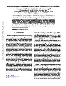
13 respect to the laboratory-fixed (or space-fixed) frame. Due to the small ratio of the electron mass to the total mass of the nuclei, ν ≈ mel . This approximation is used in the ab initio electronic structure calculations that use the electronic Hamiltonian given in Eq. (2.8) but with the ν replaced by mel . Figure 2.1 illustrates for a threenuclei, 4-electron system, the corresponding non-mass-scaled Jacobi vectors. The nuclear center of mass G is distinct from the overall system’s center of mass G. This distinction of the centers of mass and the difference between ν and mel is responsible for the so-called mass polarization effect in the electronic spectra of these systems that produces relative shifts in the energy levels of 10−4 or less. In actual scattering calculations, these differences are normally ignored as they introduce relative changes in the cross sections of the order of 10−4 or less [1]. The electronically adiabatic wave functions ψiel,ad (r; qλ ) are defined as eigenfuncb el with electronically adiabatic potential energies tions of the electronic Hamiltonian H
εad i (qλ ) as their eigenvalues:
b el (r; qλ )ψ el,ad (r; qλ ) = εad (qλ )ψ el,ad (r; qλ ) H i i i
(2.9)
The electronic Hamiltonian and the corresponding eigenfunctions and eigenvalues are independent of the orientation of the nuclear body-fixed frame with respect to the space-fixed one and hence depend only on qλ . The index i in Eq. (2.9) can span both discrete and continuous values. The ψiel,ad (r; qλ ) form a complete orthonormal basis set and satisfy the orthonormality relations δ 0 for i and i0 discrete i,i hψiel,ad (r; qλ )|ψiel,ad (r; qλ )ir = 0 δ(i − i0 ) for i and i0 continuous 0 for i discrete and i0 continuous or vice versa (2.10) These electronic wave functions are used in a Born-Huang expansion of the electronu-
clear wave function, as presented in the next section.
14
2.2
Born-Huang expansion
The total orbital wave function for this system is given by an electronically adiabatic n-state Born-Huang expansion [4, 5] in terms of this electronic basis set ψiel,ad (r; qλ ) as
Z X el,ad o χad (r; qλ ), Ψ (r, Rλ ) = i (Rλ )ψi
(2.11)
i
where
Z X
is a sum over the discrete and an integral over the continuous values of i.
i
The χad i (Rλ ), which are the coefficients in this expansion, are the adiabatic nuclear motion wave functions. The number of electronic states used in the Born-Huang expansion of Eq. (2.11) can, in most cases of interest, be restricted to a small number n of discrete states, and Eq. (2.11) replaced by Ψo (r, Rλ ) ≈
n X
el,ad χad (r; qλ ) i (Rλ )ψi
(2.12)
i=1
where n is a small number. This corresponds to restricting the motion of nuclei to only those n electronic states. In particular, if those n states constitute a sub-Hilbert space that interacts very weakly with higher states [6], this would be a very good approximation. The orbital wave function Ψo satisfies the Schr¨odinger equation
where
b int (r, Rλ )Ψo (r, Rλ ) = EΨo (r, Rλ ) H
(2.13)
b int (r, Rλ ) = Tbint (r, Rλ ) + V (r; qλ ) H
(2.14)
is the internal Hamiltonian [Eq. (2.7)] of the system that excludes the motion of its center of mass and any spin-dependent terms and E is the system’s total energy. The Eq. (2.12) through (2.14) are used next to get the n-electronic state nuclear motion Schr¨odinger equation.
15
2.2.1
Adiabatic nuclear motion Schr¨ odinger equation
Let us define χad (Rλ ) as an n-dimensional nuclear motion column vector, whose ad components are χad 1 (Rλ ) through χn (Rλ ). The n-electronic-state nuclear motion
Schr¨odinger equation satisfied by χad (Rλ ) can be obtained by inserting Eqs. (2.12) and (2.14) into (2.13) and using Eqs. (2.7) through (2.10). The resulting Schr¨odinger equation can be expressed in compact matrix form as [1] �
� � ad ad ~2 � 2 (1)ad (2)ad − I∇Rλ + 2W (Rλ ) · ∇Rλ + W (Rλ ) + ε (qλ ) − EI χ (Rλ ) = 0 , 2µ (2.15)
where I, W(1)ad , W(2)ad , and εad are n × n matrices and ∇Rλ is the column vector gradient operator in the 3(Nnu − 1)-dimensional space-fixed nuclear configuration space. I is the identity matrix and εad (qλ ) is the diagonal matrix whose diagonal elements are the n electronically adiabatic PESs εad i (qλ ) (i = 1, ..., n) being considered. All matrices appearing in this n-electronic state nuclear motion Schr¨odinger equation [Eq. (2.15)] are n-dimensional diagonal except for W (1)ad and W(2)ad , which are respectively the first- and second-derivative [1, 7–13] nonadiabatic coupling matrices discussed below. These coupling matrices allow the nuclei to sample more than one adiabatic electronic state during a chemical reaction and hence alter its dynamics in an electronically nonadiabatic fashion. It should be stressed that the effect of the geometric phase on Eqs. (2.15) must be added by either appropriate boundary conditions [1, 25] or the introduction of an appropriate vector potential [1, 14, 15].
2.2.2
First-derivative coupling matrix
The matrix W(1)ad (Rλ ) in Eq. (2.15) is an n × n adiabatic first-derivative coupling matrix whose elements are defined by (1)ad
wi,j (Rλ ) = hψiel,ad (r; qλ ) | ∇Rλ ψjel,ad (r; qλ )ir
i, j = 1, ..., n
(2.16)
16 These coupling elements are 3(Nnu − 1)-dimensional vectors. If the cartesian components of Rλ in 3(Nnu −1) space-fixed nuclear congifuration space are Xλ1 , Xλ2 , ..., Xλ3(Nnu −1) , (1)ad
the corresponding cartesian components of wi,j (Rλ ) are h
(1)ad wi,j (Rλ )
i
l
= hψiel,ad (r; qλ ) |
∂ ψiel,ad (r; qλ )ir ∂Xλl
l = 1, 2, ..., 3(Nnu − 1) (2.17)
The matrix W(1)ad is in general skew-hermitian due to Eq. (2.10) and hence its (1)ad
diagonal elements wi,i
(Rλ ) are pure imaginary quantities. If we require that the
ψiel,ad be real, then the matrix W(1)ad becomes real and skew-symmetric with the diagonal elements equal to zero and the off-diagonal elements satisfying the relation (1)ad
(1)ad
wi,j (Rλ ) = −wj,i (Rλ )
i 6= j
(2.18) (1)ad
As with any vector, the above non-zero coupling vectors (wi,j (Rλ ), i 6= j) can be decomposed, due to an extension beyond three dimensions [1] of the Helmholtz (1)ad
(1)ad
theorem [16], into a longitudinal part wi,j,lon (Rλ ) and a transverse one wi,j,tra (Rλ ) according to (1)ad
(1)ad
(1)ad
wi,j (Rλ ) = wi,j,lon (Rλ ) + wi,j,tra (Rλ ),
(2.19) (1)ad
(1)ad
where by definition, the curl of wi,j,lon(Rλ ) and the divergence of wi,j,tra (Rλ ) vanish: (1)ad
(2.20)
(1)ad
(2.21)
curl wi,j,lon (Rλ ) = 0 ∇Rλ · wi,j,tra (Rλ ) = 0
The curl in Eq. (2.20) is the skew-symmetric tensor of rank 2, whose k, l element is given by [1, 17] h
(1)ad
curl wi,j,lon (Rλ )
i
k,l
=
i i ∂ h (1)ad ∂ h (1)ad wi,j,lon (Rλ ) − wi,j,lon (Rλ ) ∂Xλl k ∂Xλk l
k, l = 1, 2, ..., 3(Nnu −1) (2.22)
17 As a result of Eq. (2.20), a scalar potential αi,j (Rλ ) exists for which (1)ad
wi,j,lon (Rλ ) = ∇Rλ αi,j (Rλ )
(2.23)
(1)ad
At conical intersection geometries, wi,j,lon(Rλ ) is singular because of the qλ dependence of ψiel,ad (r; qλ ) and ψjel,ad (r; qλ ) in the vicinity of those geometries and therefore so is the W(1)ad (Rλ ) · ∇Rλ term in Eq. (2.15). As a result of Eq. (2.19), (1)ad
W(1)ad can be written as a sum of the corresponding skew-symmetric matrices Wlon (1)ad
and Wtra , i.e., (1)ad
(1)ad
W(1)ad (Rλ ) = Wlon (Rλ ) + Wtra (Rλ )
(2.24)
This decomposition into a longitudinal and a transverse part, as will be discussed in Sec. 2.3, plays a crucial role in going to a diabatic representation in which this singularity is completely removed. In addition, the presence of the first-derivative gradient term W(1)ad (Rλ ) · ∇Rλ χad (Rλ ) in Eq. (2.15), even for a non-singular W (1)ad (Rλ ) (e.g., for avoided intersections), introduces numerical inefficiencies in the solution of that equation.
2.2.3
Second-derivative coupling matrix
The matrix W(2)ad (Rλ ) in Eq. (2.15) is an n × n adiabatic second-derivative coupling matrix whose elements are defined by (2)ad
wi,j (Rλ ) = hψiel,ad (r; qλ ) | ∇2Rλ ψjel,ad (r; qλ )ir
i, j = 1, ..., n
(2.25)
These coupling matrix elements are scalars due to the presence of the scalar laplacian ∇2Rλ in Eq. (2.25). These elements are, in general, complex but if we require the ψiel,ad to be real, they become real. The matrix W (2)ad (Rλ ), unlike its first-derivative counterpart, is neither skew-hermitian nor skew-symmetric. (2)ad
The wi,j (Rλ ) are also singular at conical intersection geometries. The decomposition of the first-derivative coupling vector, discussed in the preceding section, also
18 facilitates the removal of this singularity from the second-derivative couplings, as will be shown in Sec. 2.3. Being scalars, the second-derivative couplings can be easily included in the scattering calculations without any additional computational effort. It is interesting to note that in a one-electronic-state Born-Oppenheimer approxima(1)ad
tion, the first-derivative coupling element w1,1 (Rλ ) is rigorously zero (assuming real (2)ad
adiabatic electronic wave functions), but w1,1 (Rλ ) is not and might be important to predict sensitive quantum phenomena like resonances that can be experimentally verified.
2.3 2.3.1
Adiabatic-to-diabatic transformation Electronically diabatic representation
As mentioned at the end of Sec. 2.2.2, the presence of the W (1)ad (Rλ ) · ∇Rλ χad (Rλ ) term in the n-adiabatic-electronic-state Schr¨odinger equation [Eq. (2.15)] introduces numerical inefficiencies in its solution, even if none of the elements of the W (1)ad (Rλ ) matrix is singular. This makes it desirable to define other representations in addition to the electronically adiabatic one [Eqs. (2.9) through (2.12)], in which the adiabatic electronic wave function basis set used in the Born-Huang expansion Eq. (2.12) is replaced by another basis set of functions of the electronic coordinates. Such a different electronic basis set can be chosen so as to minimize the abovementioned gradient term. This term can initially be neglected in the solution of the n-electronic-state nuclear motion Schr¨odinger equation and reintroduced later using perturbative or other methods, if desired. This new basis set of electronic wave functions can also be made to depend parametrically, like their adiabatic counterparts, on the internal nuclear coordinates qλ that were defined after Eq. (2.8). This new electronic basis set is henceforth referred to as “diabatic” and, as is obvious, leads to an electronically diabatic representation that is not unique unlike the adiabatic one, which is unique by definition.
19 Let ψnel,d (r; qλ ) refer to that alternate basis set. Assuming that it is complete in r and orthonormal in a manner similar to Eq. (2.10), we can use it to expand the total orbital wave function of Eq. (2.11) in the diabatic version of Born-Huang expansion as
Z X o Ψ (r, Rλ ) = χdi (Rλ )ψiel,d (r; qλ ),
(2.26)
i
where the ψiel,d (r; qλ ) form a complete orthonormal basis set in the electronic coordinates and the expansion coeffecients χdi (Rλ ) are the diabatic nuclear wave functions. As in Eq. (2.12), we also usually replace Eq. (2.26) by a truncated n-term version Ψo (r, Rλ ) ≈
n X
χdi (Rλ )ψiel,d (r; qλ )
(2.27)
i=1
In the light of Eqs. (2.12) and (2.27), the diabatic electronic wave function column vector ψ el,d (r; qλ ) (with elements ψiel,d (r; qλ ), i = 1, ..., n) is related to the adiabatic one ψ el,ad (r; qλ ) (with elements ψiel,ad (r; qλ ), i = 1, ..., n) by an n-dimensional unitary transformation
where
e λ ) ψ el,ad (r; qλ ) ψ el,d (r; qλ ) = U(q
(2.28)
U† (qλ ) U(qλ ) = I
(2.29)
U(qλ ) is referred to as an adiabatic-to-diabatic transformation (ADT) matrix. Its mathematical structure is discussed in detail in Sec. 2.3.3. If the electronic wave functions in the adiabatic and diabatic representations are chosen to be real, as is normally the case, U(qλ ) is orthogonal and therefore has n(n − 1)/2 independent elements (or degrees of freedom). This transformation matrix U(qλ ) can be chosen so as to yield a diabatic electronic basis set with desired properties, which can then be used to derive the diabatic nuclear motion Schr¨odinger equation. Using Eqs. (2.27) and (2.28) and the orthonormality of the diabatic and adiabatic electronic basis sets, we can relate the adiabatic and diabatic nuclear wave functions through the same
20 n-dimensional unitary transformation matrix U(qλ ) according to e λ ) χad (Rλ ) χd (Rλ ) = U(q
(2.30)
In Eq. (2.30), χad (Rλ ) and χd (Rλ ) are the column vectors with elements χad i (Rλ ) and χdi (Rλ ), respectively, where i = 1, ..., n.
2.3.2
Diabatic nuclear motion Schr¨ odinger equation
We will assume for the moment that we know the ADT matrix of Eqs. (2.28) and (2.30) U(qλ ) and hence have a completely determined electronically diabatic basis set ψ el,d (r; qλ ). Replacing Eq. (2.27) into Eq. (2.13) and using Eqs. (2.7) and (2.8) along with the orthonormality property of ψ el,d (r; qλ ), we obtain for χd (Rλ ) the n-electronic-state diabatic nuclear motion Schr¨odinger equation �
� � d d ~2 � 2 (1)d (2)d I∇Rλ + 2W (Rλ ) · ∇Rλ + W (Rλ ) + ε (qλ ) − EI χ (Rλ ) = 0 − 2µ (2.31)
which is the diabatic counterpart of Eq. (2.15). εd (qλ ) is an n × n diabatic electronic energy matrix which in general is nondiagonal (unlike its adiabatic counterpart) and has elements defined by b el (r; qλ ) | ψ el,d (r; qλ )ir εdi,j (qλ ) = hψiel,d (r; qλ ) | H j
i, j = 1, ..., n
(2.32)
W(1)d (Rλ ) is an n × n diabatic first-derivative coupling matrix with elements defined using the diabatic electronic basis set as (1)d
wi,j (Rλ ) = hψiel,d (r; qλ ) | ∇Rλ ψjel,d (r; qλ )ir
i, j = 1, ..., n
(2.33)
Requiring ψiel,d (r; qλ ) to be real, the matrix W(1)d (Rλ ) becomes real and skewsymmetric (just like its adiabatic counterpart) with diagonal elements equal to zero. Similarly, W(2)d (Rλ ) is an n × n diabatic second-derivative coupling matrix with
21 elements defined by (2)d
wi,j (Rλ ) = hψiel,d (r; qλ ) | ∇2Rλ ψjel,d (r; qλ )ir
i, j = 1, ..., n
(2.34)
An equivalent form of Eq. (2.31) can be obtained by inserting Eq. (2.30) into Eq. (2.15). Comparison of the result with Eq. (2.31) furnishes the following relations between the adiabatic and diabatic coupling matrices: h i e λ ) ∇R U(qλ ) + W(1)ad (Rλ )U(qλ ) W(1)d (Rλ ) = U(q λ
(2.35)
h i e λ ) ∇2 U(qλ ) + 2W(1)ad (Rλ ) · ∇R U(qλ ) + W(2)ad (Rλ )U(q(2.36) W(2)d (Rλ ) = U(q ) λ Rλ λ
It also furnishes the following relation between the diagonal adiabatic energy matrix and the nondiagonal diabatic energy one: e λ )εad (qλ )U(qλ ) εd (qλ ) = U(q
(2.37)
It needs mentioning that the diabatic Schr¨odinger equation [Eq. (2.31)] also contains a gradient term W(1)d (Rλ )·∇Rλ χ(Rλ ) like its adiabatic counterpart [Eq. (2.15)]. The presence of this term can also introduce numerical inefficiency problems in the solution of Eq. (2.31). Since the ADT matrix U(qλ ) is arbitrary, it can be chosen to make Eq. (2.31) have desirable properties that Eq. (2.15) doesn’t possess. U(q λ ) can, for example, be chosen so as to automatically minimize W (1)d (Rλ ) relative to W(1)ad (Rλ ) everywhere in internal nuclear configuration space and incorporate the effect of the geometric phase. Next we will consider the structure of this ADT matrix for an n-electronic-state problem and a general evaluation scheme that minimizes the magnitude of W(1)d (Rλ ).
22
2.3.3
Diabatization matrix
In the n-electronic-state adiabatic representation involving real electronic wave functions, the skew-symmetric first-derivative coupling vector matrix W (1)ad (Rλ ) has (1)ad
n(n − 1)/2 independent non-zero coupling vector elements wi,j (Rλ ), (i 6= j). The ones having the largest magnitudes are those that couple adjacent neighboring adi(1)ad
abatic PESs, and therefore the dominant wi,j (Rλ ) are those for which j = i ± 1, i.e., lying along the two off-diagonal lines adjacent to the main diagonal of zeroes. (1)ad
Each one of the wi,j (Rλ ) elements is associated with a scalar potential αi,j (Rλ ) through their longitudinal component (see Eqs. (2.19) and (2.23)). A convenient and general way of parametrizing the n × n orthogonal ADT matrix U(qλ ) of Eqs. (2.28) (1)ad
and (2.30) is as follows. Since the coupling vector element wi,j (Rλ ) couples the electronic states i and j, let us define an n × n orthogonal i, j-diabatization matrix (ui,j (qλ ), with j > i) whose row k and column l element (k, l = 1, 2, ..., n) is designated by uk,l i,j (qλ ) and is defined in terms of a set of diabatization angles βi,j (qλ ) by the relations uk,l i,j (qλ ) =
cos βi,j (qλ )
for k = i and l = i
=
cos βi,j (qλ )
for k = j and l = j
= − sin βi,j (qλ )
for k = i and l = j
=
sin βi,j (qλ )
for k = j and l = i
=
1
for k = l 6= i or j
=
0
for the remaining k and l
(2.38)
This choice of elements for the ui,j (qλ ) matrix will diabatize the adiabatic electronic states i and j while leaving the remaining states unaltered. As an example, in a 4-electronic-state problem (n = 4) consider the electronic states i = 2 and j = 4 along with the first-derivative coupling vector element (1)ad
w2,4 (Rλ ) that couples those two states. The ADT matrix u2,4 (qλ ) can then be
23 expressed in terms of the corresponding diabatization angle β2,4 (qλ ) as
1
0
0
0
0 cos β2,4 (qλ ) 0 − sin β2,4 (qλ ) u2,4 (qλ ) = 0 0 1 0 0 sin β2,4 (qλ ) 0 cos β2,4 (qλ )
(2.39)
This diabatization matrix only mixes the adiabatic states 2 and 4 leaving the states 1 and 3 unchanged. In the n-electronic-state case, n(n − 1)/2 such matrices ui,j (qλ ) (j > i with i = 1, 2, ..., n − 1 and j = 2, ..., n) can be defined using Eq. (2.38). The full ADT matrix U(qλ ) is then defined as a product of these n(n − 1)/2 matrices ui,j (qλ ) (j > i) as
U(qλ ) =
n−1 Y
n Y
ui,j (qλ )
(2.40)
i=1 j=i+1
which is the n-electronic-state version of the expression that has appeared earlier [18, 19] for three electronic states. This U(qλ ) is orthogonal, as it is the product of orthogonal matrices. The matrices ui,j (qλ ) in Eq. (2.40) can be multiplied in any order without loss of generality. A different multiplication order leads to a different set of solutions for the diabatization angles βi,j (qλ ). However, since the matrix U(qλ ) is a solution of a set of Poisson-type equations with fixed boundary conditions, as will be discussed next, it is uniquely determined and therefore independent of this choice of the order of multiplication, i.e., all of these sets of βi,j (qλ ) give the same U(qλ ) [19]. It should be remembered, however, that these are purely formal considerations, which are useful for the truncated Born-Huang expansion as discussed after Eq. (2.46). We want to choose the ADT matrix U(qλ ) that either makes the diabatic firstderivative coupling vector matrix W (1)d (Rλ ) zero if possible or that minimizes its magnitude in such a way that the gradient term W (1)d (Rλ ) · ∇Rλ χd (Rλ ) in Eq. (2.31) can be neglected. Rewriting the relation between W (1)d (Rλ ) and W(1)ad (Rλ ) of
24 Eq. (2.35) as � � e λ ) ∇R U(qλ ) + W(1)ad (Rλ )U(qλ ) W(1)d (Rλ ) = U(q λ
(2.41)
we see that all elements of the diabatic matrix W (1)d (Rλ ) will vanish if and only if all elements of the matrix inside the square brackets in the right-hand side of this equation are zero, i.e., ∇Rλ U(qλ ) + W(1)ad (Rλ )U(qλ ) = 0
(2.42)
The structure of W(1)ad (Rλ ) discussed at the beginning of this section, will reflect itself in some interrelations between the βi,j (qλ ) obtained by solving this equation. More importantly, this equation has a solution if and only if the elements of the matrix W(1)ad (Rλ ) satisfy the following curl-condition [1, 20–23] for all values of Rλ : h
(1)ad
curl wi,j (Rλ )
i
k,l
(1)ad
In this equation, wp
i h (1)ad (1)ad = − wk (Rλ ), wl (Rλ )
i,j
k, l = 1, 2, ..., 3(Nnu − 1) (2.43)
(Rλ ) (with p = k, l) is the n×n matrix whose row i and column (1)ad
(1)ad
j element is the p cartesian component of the wi,j (Rλ ) vector, i.e., [wi,j (Rλ )]p , and the square bracket on its right-hand side is the commutator of the two matrices within. This condition is satisfied for an n × n matrix W (1)ad (Rλ ) when n samples the complete infinite set of adiabatic electronic states. In that case, we can rewrite Eq. (2.42) using the unitarity property [Eq. (2.29)] of U(qλ ) as e λ ) = −W(1)ad (Rλ ) [∇Rλ U(qλ )] U(q
(2.44)
This matrix equation can be expressed in terms of individual matrix elements on both sides as
X� k
� (1)ad ∇Rλ fi,k [β(qλ )] fj,k [β(qλ )] = −wi,j (Rλ )
(2.45)
where β(qλ ) ≡ (β1,2 (qλ ), ..., β1,n (qλ ), β2,3 (qλ ), ..., β2,n (qλ ), ..., βn−1,n (qλ )) is a set of all
25 unknown diabatization angles and fp,q [β(qλ )] with p, q = i, j, k are matrix elements of the ADT matrix U(qλ ), which are known trigonometric functions of the unknown β(qλ ) due to Eqs. (2.38) and (2.40). Equations (2.45) are a set of coupled first-order partial differential equations in the unknown diabatization angles βi,j (qλ ) in terms of (1)ad
the known first-derivative coupling vector elements wi,j (Rλ ) obtained from ab initio electronic structure calculations [7]. This set of coupled differential equations can be solved in principle with some appropriate choice of boundary conditions for the angles βi,j (qλ ). The ADT matrix U(qλ ) obtained in this way makes the diabatic first-derivative coupling matrix W(1)d (Rλ ) that appears in the diabatic Schr¨odinger equation [Eq. (2.31)] rigorously zero. It also leads to a diabatic electronic basis set that is independent of qλ [23], which, in agreement with the present formal considerations, can only be a correct basis set if it is complete, i.e., infinite. It can be proved using Eqs. (2.35), (2.36) and (2.42) that this choice of the ADT matrix also makes the diabatic secondderivative coupling matrix W (2)d (Rλ ) appearing in Eq. (2.31) equal to zero. As a result, when n samples the complete set of adiabatic electronic states, the corresponding diabatic nuclear motion Schr¨odinger equation [Eq. (2.31)] reduces to the simple form
� � 2 � d d ~ 2 − I∇Rλ + ε (qλ ) − EI χ (Rλ ) = 0 2µ
(2.46)
where the only term that couples the diabatic nuclear wave functions χd (Rλ ) is the diabatic energy matrix εd (qλ ). The curl-condition given by Eq. (2.43) is in general not satisfied by the n × n matrix W(1)ad (Rλ ), if n doesn’t span the full infinite basis set of adiabatic electronic states and is truncated to include only a finite small number of these states. This truncation is extremely convenient from a physical as well as computational point of view. In this case, since Eq. (2.42) does not have a solution, let us consider instead the equation obtained from it by replacing W (1)ad (Rλ ) by its longitudinal part: (1)ad
∇Rλ U(qλ ) + Wlon (Rλ )U(qλ ) = 0
(2.47)
26 This equation does have a solution, because in view of Eq. (2.20) the curl condition (1)ad
of Eq. (2.43) is satisfied when W (1)ad (Rλ ) is replaced by Wlon (Rλ ). We can now rewrite Eq. (2.47) using the orthogonality of U(qλ ) as e λ ) = −W(1)ad (Rλ ) [∇Rλ U(qλ )] U(q lon
(2.48)
The quantity on the right-hand side of this equation is not completely specified since the decomposition of W(1)ad (Rλ ) into its longitudinal and transverse parts given by Eq. (2.24) is not unique. Using that decomposition and the property of the transverse (1)ad
part Wtra (Rλ ) given by Eq. (2.21), we see that (1)ad
∇Rλ · Wlon (Rλ ) = ∇Rλ · W(1)ad (Rλ )
(2.49) (1)ad
and since W(1)ad (Rλ ) is assumed to have been previously calculated, ∇Rλ ·Wlon (Rλ ) is known. If we take the divergence of both sides of Eq. (2.48), we obtain (using Eq. (2.49)) h i � 2 � e e ∇Rλ U(qλ ) U(qλ ) + [∇Rλ U(qλ )] · ∇Rλ U(qλ ) = −∇Rλ · W(1)ad (Rλ )
(2.50)
Using the parameterization of U(qλ ) given by Eqs. (2.38) and (2.40) for a finite n, this matrix equation can be expressed in terms of the matrix elements on both sides as X �� k
∇2Rλ fi,k [β(qλ )]
�
�� �� (1)ad fj,k [β(qλ )]+ ∇Rλ fi,k [β(qλ )] · ∇Rλ fj,k [β(qλ )] = −∇Rλ ·wi,j (Rλ ) �
(2.51)
where fp,q are the same as defined after Eq. (2.45). Equation (2.51) is a set of coupled Poisson-type equations in the unknown angles βi,j (qλ ). For n = 2 this becomes Eq. (4.30), as shown in Chapter 4. The structure of this set of equations is again dependent on the order of multiplication of matrices ui,j (qλ ) in Eq. (2.40). Each choice of the order of multiplication will give a different set of βi,j (qλ ) as before but
27 the same ADT matrix U(qλ ) after they are solved using the same set of boundary conditions. Using the fact that for a finite number of adiabatic electronic states n, we choose a U(qλ ) that satisfies Eq. (2.47) (rather than Eq. (2.42) that has no solution), Eq. (2.35) now reduces to e λ )Wtra (Rλ )U(qλ ) W(1)d (Rλ ) = U(q (1)ad
(2.52)
This can be used to rewrite the diabatic nuclear motion Schr¨odinger equation for an incomplete set of n electronic states as �
� o � d ~2 n 2 (1)ad (2)d d e λ )Wtra (Rλ )U(qλ ) · ∇R + W (Rλ ) + ε (qλ ) − EI χ (Rλ ) = 0 − I∇Rλ + 2U(q λ 2µ (2.53)
e λ )Wtra (Rλ )U(qλ )·∇R χd (Rλ ) = W(1)d (Rλ )· In this equation, the gradient term U(q λ (1)ad
∇Rλ χd (Rλ ) still appears and, as mentioned before, introduces numerical inefficiencies
in its solution. Even though a truncated Born-Huang expansion was used to obtain (1)ad
Eq. (2.53), Wtra (Rλ ), although no longer zero, has no poles at conical intersection geometries (as opposed to the full W (1)ad (Rλ ) matrix). The set of coupled Poisson equations [Eq. (2.50)] can, in principle, be solved with any appropriate choice of boundary conditions for βi,j (qλ ). There is one choice, (1)ad
however, for which the magnitude of Wtra (Rλ ) is minimized. If at the boundary surfaces Rbλ of the nuclear configuration space spanned by Rλ (and the corresponding subset of boundary surfaces qbλ in the internal configuration space spanned by qλ ), one imposes the following mixed Dirichlet-Neumann condition (based on Eq. (2.48)), h
∇Rbλ U(qbλ )
i
e b ) = −W(1)ad (Rb ) U(q λ λ
(2.54)
it minimizes the average magnitude of the vector elements of the transverse coupling (1)ad
matrix Wtra (Rλ ) over the entire internal nuclear configuration space and hence the magnitude of the gradient W(1)d (Rλ ) · ∇Rλ χd (Rλ ), as will be shown for the n = 2 case [24] in Chapter 4. To a first very good approximation, this term can be neglected
28 in the diabatic Schr¨odinger Eq. (2.53) resulting in a simpler equation � 2 � � d d ~ � 2 (2)d − I∇Rλ + W (Rλ ) + ε (qλ ) − EI χ (Rλ ) = 0 2µ
(2.55)
In this diabatic Schr¨odinger equation, the only terms that couple the nuclear wave functions χdi (Rλ ) are the elements of the W(2)d (Rλ ) and εd (qλ ) matrices.
The
2
~ W(2)d (Rλ ) matrix does not have poles at conical intersection geometries (as op− 2µ
posed to W(2)ad (Rλ )) and furthermore it only appears as an additive term to the diabatic energy matrix εd (qλ ) and doesn’t increase the computational effort for the solution of Eq. (2.55). Since the neglected gradient term is expected to be small, it can be reintroduced as a first order perturbation afterwards, if desired. In the following chapters, this theory will be applied to a two-electronic-state triatomic problem and results presented for the H3 system.
29
Bibliography [1] A. Kuppermann, in Dynamics of Molecules and Chemical Reactions, edited by R. E. Wyatt and J. Z. H. Zhang (Marcel Dekker, New York, 1996), pp. 411-472. [2] L. M. Delves, Nucl. Phys. 9, 391 (1959). [3] L. M. Delves, Nucl. Phys. 20, 275 (1960). [4] M. Born, Nachr. Akad. Wiss. G¨ott. Math.-Phys. Kl. Article No. 6, 1 (1951). [5] M. Born and K. Huang, Dynamical Theory of Crystal Lattices (Oxford University Press, Oxford, 1954), pp. 166-177 and 402-407. [6] M. Baer, Chem. Phys. Lett. 322, 520 (2000). [7] B. H. Lengsfield and D.R. Yarkony, in State-selected and State-to-State IonMolecule Reaction Dynamics: Part 2 Theory, Vol. 82, edited by M. Baer and C.-Y. Ng (Wiley, New York, 1992), pp. 1-71. [8] R. J. Buenker, G. Hirsch, S. D. Peyerimhoff, P. J. Bruna, J. R¨omelt, M. Bettendorff, and C. Petrongolo, in Current Aspects of Quantum Chemistry, Elsevier, New York, 1981, pp. 81-97. [9] M. Desouter-Lecomte, C. Galloy, J. C. Lorquet, and M. V. Pires, J. Chem. Phys. 71, 3661 (1979). [10] B. H. Lengsfield, P. Saxe, and D. R. Yarkony, J. Chem. Phys. 81, 4549 (1984). [11] P. Saxe, B. H. Lengsfield, and D. R. Yarkony, Chem. Phys. Lett. 113, 159 (1985). [12] B. H. Lengsfield, and D. R. Yarkony, J. Chem. Phys. 84, 348 (1986). [13] J. O. Jensen and D. R. Yarkony, J. Chem. Phys. 89, 3853 (1988).
30 [14] C. A. Mead and D. G. Truhlar, J. Chem. Phys. 70, 2284 (1979). [15] B. Kendrick and R. T. Pack, J. Chem. Phys. 104, 7475 (1996). [16] P. M. Morse and H. Feshbach, Methods of Theoretical Physics (McGraw-Hill, New York, 1953), pp. 52-54, 1763. [17] H. Margenau and G. M. Murphy, The Mathematics of Physics and Chemistry (Van Nostrand, New York, 1943), p. 192. [18] M. Baer (Ed.), Theory of Chemical Reaction Dynamics Vol. II, (CRC Press, Boca Raton (Florida), 1985), chapter 4. [19] A. Alijah and M. Baer, J. Phys. Chem. A 104, 389 (2000). [20] M. Baer and R. Englman, Mol. Phys. 75, 293 (1992). [21] M. Baer, Chem. Phys. Lett. 35, 112 (1975). [22] M. Baer, Chem. Phys. 15, 49 (1976). [23] C. A. Mead and D. G. Truhlar, J. Chem. Phys. 77, 6090 (1982). [24] R. Abrol and A. Kuppermann, J. Chem. Phys. 116, 1035 (2002). [25] Y.-S. M. Wu, A. Kuppermann, and B. Lepetit, Chem. Phys. Lett. 186, 319 (1991).
31
Figure 2.1: Jacobi vectors for a three-nuclei, four-electron system. The nuclei are P 1 , P2 , P3 and the electrons are e1 , e2 , e3 , e4 .
32
Chapter 3
Accurate first-derivative
nonadiabatic couplings for H3 system 3.1
Introduction
For any polyatomic system involving three or more atoms, the ground and the firstexcited adiabatic electronic PESs can intersect even if the corresponding states have the same symmetry and spin multiplicity [1]. These intersections, which are usually conical, occur quite frequently in polyatomic systems. The reason is that these polyatomic systems possess three or more internal nuclear motion degrees of freedom, and only two independent relations between three electronic Hamiltonian matrix elements are sufficient for the existence of doubly degenerate electronic energy eigenvalues. As a result, these relations between those matrix elements are easily satisfied and explain the frequent occurrence of conical intersections. Assuming the adiabatic electronic wave functions to be real and as continuous as possible in the nuclear coordinate space, if the polyatomic system is transported around a closed loop in that space (a so-called pseudorotation) that encircles a conical intersection geometry, these electronic wave functions must change sign [1,2]. This change of sign has consequences for the structure and dynamics of the polyatomic system, as it requires the corresponding nuclear wave functions to undergo a compensatory change of sign, known as the geometric phase (GP) effect [3–7], to keep the total wave function single-valued. This sign change is a special case of Berry’s geometric phase [6], and is also referred to as the molecular Aharonov-Bohm effect [8]. It greatly affects the nature of the solutions of the corresponding nuclear motion Schr¨odinger equation [7, 9]. Accurate quantummechanical reactive scattering calculations (on the ground electronic PES), with and without the GP effect included, have been carried out for the H + H2 system and
33 its isotopic variants (D + H2 and H + D2 ) [9–13] to obtain differential and integral cross sections. The cross sections obtained with the GP effect included were in much better agreement with the experimental results [14–17] than those obtained with the GP effect excluded. Hence, the GP effect is an important factor in accurate quantum scattering calculations done on the ground adiabatic electronic PES. A review of the one- and two-electronic-state Born-Huang [18, 19] (also usually called Born-Oppenheimer) approximations has been given in detail elsewhere [7] and only the features pertinent to this chapter are summarized here. In the one-electronicstate approximation, the GP effect has to be imposed on the adiabatic nuclear wave functions in order to obtain accurate results at low energies. At energies above the conical intersection energy, when this approximation breaks down, the effect of the first-excited electronic PES has to be included explicitly in the scattering calculations to obtain accurate results. In the adiabatic representation, the GP effect still has to be imposed on each of the two state nuclear wave functions. In this two-electronic-state approximation [7], the nuclear motion Schr¨odinger equation for an N -atom system [Eq. (2.15)] becomes � 2 � � ad ad ~ � 2 (1)ad (2)ad − I∇Rλ + 2W (Rλ ) · ∇Rλ + W (Rλ ) + ε (qλ ) − EI χ (Rλ ) = 0, 2µ (3.1) where Rλ is a set of 3(N − 1) nuclear coordinates (remaining after the removal of the center of mass coordinates), and qλ is a set of 3(N − 2) internal nuclear coordinates obtained by removing from the set Rλ three Euler angles which orient a nuclear bodyfixed frame with respect to a space-fixed one. As an example, for a triatomic system Rλ can be a set of principal axes of inertia body-fixed symmetrized hyperspherical coordinates (ρ, θ, φλ , aλ , bλ , cλ ) [7, 9], and qλ is then comprised of ρ, θ, and φλ since the remaining aλ , bλ , cλ , are Euler angles. It is shown in Appendix 3.A that for a triatomic system, W(1)ad (Rλ ) · ∇Rλ of Eq. (3.1) can be replaced by W (1)ad (qλ ) · ∇Rλ . The matrix W(2)ad (Rλ ) can also be replaced by W(2)ad (qλ ) as the electronic wave functions don’t depend on the three Euler angles mentioned above. So Eq. (3.1)
34 becomes � 2 � � ad ad ~ � 2 (1)ad (2)ad − I∇Rλ + 2W (qλ ) · ∇Rλ + W (qλ ) + ε (qλ ) − EI χ (Rλ ) = 0 2µ (3.2) In addition, I is a 2 × 2 identity matrix,
χad (Rλ ) =
χad 1 (Rλ ) χad 2 (Rλ )
(3.3)
is a 2×1 column vector whose elements are the ground (χad 1 (Rλ )) and the first-excited (χad 2 (Rλ )) adiabatic nuclear motion wave functions, and
εad (qλ ) =
εad 1 (qλ )
0
0
εad 2 (qλ )
(3.4)
is a diagonal matrix whose diagonal elements are the ground (εad 1 (qλ )) and the firstexcited (εad 2 (qλ )) adiabatic electronic PESs. W(1)ad (qλ ) and W(2)ad (qλ ) are respectively the first-derivative [20–23] and secondderivative [20, 24, 25] nonadiabatic coupling matrix elements between the ground and first-excited adiabatic electronic PESs. For the two-electronic-state approximation they are 2 × 2 matrices, whose elements are defined by (1)ad ad Wm,n (qλ ) = hψm (r; qλ ) | ∇Rλ ψnad (r; qλ )ir ad 2 ad W(2)ad m,n (qλ ) = hψm (r; qλ ) | ∇Rλ ψn (r; qλ )ir ,
and
(3.5) (3.6)
where r is a set of electronic coordinates, and m and n refer to the ground or the firstexcited electronic PESs. ψnad (r; qλ ) is an eigenfunction of the electronic Hamiltonian and satisfies the electronic Schr¨odinger equation h
i ˆ el − εad (qλ ) ψ ad (r; qλ ) = 0. H n n
(3.7)
35 ψnad (r; qλ ) and εad n (qλ ) depend only on the internal nuclear coordinates qλ because the coulombic interaction potential between the (N -atom) system’s particles (nuclei ˆ el , depends only on their relative distances and and electrons), which appears in H hence these quantities depend on qλ but not on the three Euler angles which orient the nuclear frame with respect to a space-fixed one. This introduces small rotational coupling terms that are two orders of magnitude or more smaller than the remaining coupling terms and can be neglected. This leads to a subtle but important point implicit in Eqs. (3.5) and (3.6): although the right-hand sides of these equations contain Rλ , the left-hand sides contain only qλ . Also, since ∇Rλ and ∇2Rλ are respectively (1)ad
the gradient and laplacian operators, Wm,n (qλ ) is a vector quantity and W(2)ad m,n (qλ ) is a scalar quantity. The matrix W(1)ad (qλ ) is skew-hermitian, and if we choose ψ1ad (r; qλ ) and ψ2ad (r; qλ ) (1)ad
(1)ad
to be real, it is skew-symmetric and W1,1 (qλ ) and W2,2 (qλ ) are identically zero. (1)ad
(1)ad
Furthermore, the off-diagonal elements, W1,2 (qλ ) and W2,1 (qλ ), satisfy the relation (1)ad
(1)ad
W1,2 (qλ ) = −W2,1 (qλ ).
(3.8)
The presence of the first-derivative term W (1)ad (qλ ) · ∇Rλ in Eq. (3.2) introduces inefficiencies in the numerical solution of this equation. A diabatic representation [7,26] of this equation is introduced to circumvent this problem, since in that representation the first-derivative coupling element is minimized. It has been shown [27, 28] that in general a perfect diabatic basis that makes that first term vanish for all nuclear geometries does not exist for a polyatomic system, and hence a finite part of the first-derivative coupling cannot be totally removed even in the diabatic representation. This part is referred to in literature as the nonremovable part. For systems (1)ad
having a conical intersection, W1,2 (qλ ) has a singularity at conical intersection geometries [29]. This singularity along with some finite part of the coupling is removable upon an adiabatic to diabatic transformation and is hence referred to as the removable part. Mead and Truhlar [28] have shown how to calculate the removable part, but their approach is difficult to implement [30]. Over the years, a number of formalisms
36 involving (quasi-)diabatic basis have also been put forward [30–40]. This chapter focuses on the calculation of high-quality ab initio ground and firstexcited electronic energies and the first-derivative couplings between them. The second-derivative couplings are generally assumed to be negligible as compared to the other terms in the Hamiltonian [Eq. (3.2)], except at the conical intersection [41]. These accurate energies and first-derivative couplings will be used for transforming the two-state adiabatic problem expressed by Eq. (3.2) to a (quasi-)diabatic representation and will be incorporated into the quantum scattering formalism to calculate the effect of conical intersections on the dynamics of the chemical reactions at energies for which a minimum of two electronic states is required to obtain accurate results. The H + H2 system is being used for this work because it is the simplest of the chemical reactions for which the concurrent bond breaking and bond formation can be studied in detail both experimentally and theoretically. Many quantum scattering calculations have been performed on this system [9,10,42–45]. The equilateral triangle (C3v ) configuration of H3 corresponds to a conical intersection between the ground and the first-excited electronic states of the system. This conical intersection induces a GP that is important in studying the reactive scattering in the ground state [7, 9–13, 46, 47]. With the breakdown of the one electronic state Born-Oppenheimer approximation near 2.75 eV, which corresponds to the minimum of the first-excited PES [48], both surfaces must be used in a scattering calculation for an accurate result to be obtained. Such two-state calculations should be performed and compared with the recent quantum scattering calculations [9,10] done with and without the inclusion of the GP effect. This comparison is expected to provide an upper limit to the energy at which the ground state PES by itself, with an incorporation of the GP effect, is capable of furnishing a quantitative description of the reaction dynamics of the H3 system and its isotopomers. In this chapter, we present the first-derivative nonadiabatic couplings between the ground and the first-excited PESs for the H + H2 system obtained from high-quality ab initio wave functions and analytic gradient techniques over the entire nuclear
37 internal configuration space. We also present a fit to the corresponding ground and first-excited electronic PESs and analyze the regions of that space for which the first-derivative couplings could affect the dynamics of the H + H2 reaction. For comparison, we also present the first-derivative couplings and the lowest two electronic PESs obtained analytically from the double many-body expansion (DMBE) method of Varandas et al. [49], as the DMBE couplings are designed to be accurate only in the vicinity of the conical intersection. In Sec. 3.2, we describe the methods used to obtain the first-derivative couplings and introduce their contour integrals. In Sec. 3.3, we present a fit to the ab initio energies corresponding to the lowest two electronic PESs and compare them to the DMBE ones. We present and compare the ab initio and DMBE first-derivative couplings in Sec. 3.4, which is concluded by an analysis of the contour integrals of the ab initio couplings.
3.2 3.2.1
Theory and numerical methods Ab initio couplings and electronic energies
The first-derivative couplings are determined using an analytic gradient technique summarized in Ref. [50]. This technique is a significant improvement over the finitedifference techniques introduced previously [20, 51–54] and has been used recently in a number of problems to obtain electronic energies and first-derivative couplings [37, 55–58]. Using it, the first-derivative couplings are first evaluated in terms of six atom-centered displacements [50] in the H3 molecular plane and then transformed to standard internal mass-scaled Jacobi coordinates (Rλ , rλ , γλ ). In addition to the derivative couplings associated with these coordinates, the coupling due to rotation in the molecular plane is also determined. This rotational coupling must equal the interstate matrix element of the z component of total electronic orbital angular momentum operator, Lez [59, 60]. This equivalence provides a measure of the precision
38 of the derivative couplings presented in this chapter and the two approaches agree to 1 × 10⁻⁶ bohr−1 . In this work, the first-derivative couplings and the ground (E1 ) and first-excited (E2 ), electronic PESs for H3 were determined on a grid of 784 geometry points picked in the symmetrized hyperspherical coordinates (qλ :ρ, θ, φλ ) used previously [7, 9] and defined in detail in Sec. 3.3. The adiabatic wave functions, first-derivative couplings, and electronic energies were determined from second-order CI [61–63] wave functions based on a three-electron, three-orbital, active space. The molecular orbitals were determined from a complete active space [64–66] state-averaged multiconfiguration self-consistent field procedure [67, 68], in which two 2 A0 states were averaged with weights (0.505,0.495) based on (6s3p1d) contracted Gaussian basis sets on the hydrogens. After being evaluated in nuclear mass-scaled Jacobi coordinates as mentioned above, the first-derivative couplings are transformed to the qλ coordinates (ρ, θ, φλ ) to obtain the first-derivative coupling vector (1)ad
W1,2 (qλ ) = hψ1ad (r; qλ ) | ∇qλ ψ2ad (r; qλ )ir ,
(3.9)
whose components in the ρ, θ and φλ unit vector directions are defined as ∂ ad ψ (r; ρ, θ, φλ )ir , ∂ρ 2 1 ∂ ad (1)ad ψ (r; ρ, θ, φλ )ir , and W1,2,θ (ρ, θ, φλ ) = hψ1ad (r; ρ, θ, φλ ) | ρ ∂θ 2 1 ∂ ad (1)ad W1,2,φλ (ρ, θ, φλ ) = hψ1ad (r; ρ, θ, φλ ) | ψ (r; ρ, θ, φλ )ir . ρ sin θ ∂φλ 2 (1)ad
W1,2,ρ (ρ, θ, φλ ) = hψ1ad (r; ρ, θ, φλ ) |
(3.10) (3.11) (3.12)
The values of the qλ coordinates (ρ, θ, φλ ) are limited to the ranges 0≤ρ