Furthermore during the chemical reaction work may also be done work in ... The total number of moles of substrates and products may not be equal, for .... formula (2.9), need not be the same as those found at the end of the equations. The ..... pressures of all the reactants are equal to unity. Lmax ¼ ÐR Ð T ln K ¼. X i vil0 i.
Chapter 2
Theory
2.1 Thermodynamic Background Thermodynamics is the science that studies the processes of energy conversion from one form to another. Most of these changes are performed to obtain energy in the shape of heat or work (which may be mechanical or electrical). The power source used is mostly fuel, in which energy is trapped in the form of chemical bonds between atoms. Release and subsequent use of this energy can be made using a heat engine (usually working in the cycle of heat—internal combustion engines, turbines) or fuel cell. In the case of a heat engine, the chemical energy of fuel is released as heat and mechanical energy produced through other processes. Mechanical energy is then converted into electricity using electro-magnetic devices (generators). Thermodynamic laws restrict the amount of energy that can be obtained in the process of conversion, but the global energy balance is always zero (except in nuclear processes). Thermodynamic analysis of fuel cells and thermal cycles shows that processes taking place at a constant temperature are more efficient than processes taking place at highly variable temperatures.
2.1.1 Thermal Effect of Chemical Reaction Chemical reactions are usually associated with certain effects of energy, which can be emitted or absorbed, and are therefore categorized as exothermic or endothermic reactions. Furthermore during the chemical reaction work may also be done work in forms that are not only mechanical, but electrical, magnetic, etc. Accordingly, chemical reactions are often thermodynamic transformations and can be analyzed by thermodynamic methods. J. Milewski et al., Advanced Methods of Solid Oxide Fuel Cell Modeling, Green Energy and Technology, DOI: 10.1007/978-0-85729-262-9_2, � Springer-Verlag London Limited 2011
17
18
2 Theory
A chemical reaction can be written symbolically in the following form: aA þ bB þ � � � kK þ lL þ � � �
ð2:1Þ
where: a; b; . . .; k; l; . . . mean the number of moles of individual substances A; B; . . .; K; L; . . . involved in chemical reactions and are called stoichiometric coefficients. 1 H2 þ O2 ! H2 O ð2:2Þ 2 The total number of moles of substrates and products may not be equal, for instance (2.2), in which 1.5 kmol of hydrogen and oxygen formed 1 kmol of water. However, according to the principle of mass conservation the following condition must be fulfilled: aMA þ bMB þ � � � ¼ kMK þ lML þ � � �
ð2:3Þ
where MA ; MB ; . . . mean molecular weights of the individual substances A; B; . . .. This equation can be written symbolically in the following form: X vi � M i ¼ 0 ð2:4Þ where vi mean stoichiometric ratios, and Mi appropriate molecular weights, but introduced an additional convention that the value of vi on the left side of reaction (2.4) are positive, but negative on the right. This convention will be applied consistently in this book because of the convenience and simplicity of writing the reactions. As mentioned previously, chemical reactions are generally associated with generation or absorption of heat, while in chemical thermodynamics, generated heat is mostly indicated by a positive sign, whereas absorbed heat by a negative sign. To maintain uniformity throughout the text, the opposite indication is used, i.e. emitted heat is negative, absorbed heat is positive. A reaction heat is called the largest possible amount of heat generated or absorbed during the reaction, assuming that the transformation takes place in isothermal conditions, and that also a constant value is kept for one of the parameters: pressure or volume. Therefore, a distinction is made between heat of reaction for an isochoric–isothermal (Qv ) or isobaric–isothermal (Qp ) reaction. They differ from each other, but are referred to as 1 kmol or 1 kg. In accordance with the aforementioned signs for indicating the heat effects of reaction, the value of Qv can be calculated from the relationship: Qv ¼ U2 � U1
ð2:5Þ
Similarly, the heat of reaction at constant pressure: Qp ¼ U2 � U1 þ p
Z2 1
dV ¼ U2 � U1 þ pV2 � pV1 ¼ I2 � I1
ð2:6Þ
2.1 Thermodynamic Background
19
The difference between Qp and Qv is Qp � Qv ¼ U2 � U1 þ p � ðV2 � V1 Þ � ðU2 � U1 Þ ¼ p � ðV2 � V1 Þ ¼ p � DV ð2:7Þ Since the values of U1 ; I1 ; U2 , and I2 are the internal energy and enthalpy of substrates (U1 ; I1 ) and products (U2 ; I2 ), they represent the sum of the internal energy and enthalpy of substances that are substrates and products of the reaction. Heat of reaction in general depends on temperature and pressure and, therefore, the normal (standard) state is amended as a contractual condition in order to clearly determine the heat needed to create chemical compounds. The heat effect occurring at standard conditions is called the heat of formation. The standard state usually means a temperature of 25�C and pressure of 0.098 MPa. The appropriate values are indicated by 298, which denotes the reference temperature (298 K). Moreover, it is assumed that each of the reactants involved in the reactions occur in the stable form typical for its physical state at the standard conditions. As the heat of reaction at constant volume is equal to the difference between internal energy at the beginning and the end of the transformation, and the effect of reaction heat at constant pressure is equal to the difference between enthalpy at the beginning and the end of the transformation, respectively; the heat of reaction is independent of the pathway, and is only a function of the initial and final state. This proposal is called Hess’s law, which enables the indirect determination of the total heat effect of the reactions chain by knowing separately the reaction heats for each reaction in the chain. For example Eq. 2.7 can be written in the following form: Qp ¼ k � IK þ l � IL � a � IA � b � IB
ð2:8Þ
where IK ; IL ; IA and IB mean molar enthalpy of bodies K; L; A and B from the reaction described by the relation (2.1). To find the true value of Qp , the molar enthalpy must be properly calculated. This is crucial because in general total enthalpy is difficult to determine, and is usually calculated from a reference state in which it is assumed as equal to zero. This assumption is non-problematic so long as the conversion of chemical reactions remains unconnected with the disappearance of some substances and the formation of others. Difficulties arise with chemical reactions in terms of the adoption of zero enthalpy for each of the reactants. The equation for Qp can also be written as: Qp ¼k � ðIK � IK0 Þ þ l � ðIL � IL0 Þ � a � ðIA � IA0 Þ � b � ðIB � IB0 Þ þ ðk � IK0 þ l � IL0 � a � IA0 � b � IB0 Þ where the symbols IK0 ; IL0 ; IA0 ; IB0 label reagents in molar enthalpy at the standard state. It is worth mentioning that the standard enthalpy, found in brackets in the
20
2 Theory
formula (2.9), need not be the same as those found at the end of the equations. The individual values in the brackets do not depend on what state adopted zero enthalpy, because it contains only the differences in enthalpy in two different states for the same component. The values of I 0 in the last segment of the formula (2.9) must be chosen in an appropriate way to achieve the right result. For this reason the value of heat of formation at the standard state is defined. The standard heat of formation is the thermal effect of an isothermal–isobaric reaction which synthesizes the products from basic components at standard state conditions. In addition, it is assumed that the heat of formation of the standard elements is found in most permanent states of concentration at standard conditions (although it sometimes departs from this assumption.) Generally, it is accepted that the value of enthalpy of the elements at the standard state is zero. Use of these assumptions enables the calculation of standard heat of formation for all components. The resulting values are summarized in chemical tables and can be used in the calculations. A similar approach could also provide a thermal effect Qv enthalpy with the difference that it is based on internal energies (instead of enthalpies).
2.1.2 Kirchhoff Equations Looking at the isothermal–isobaric or isothermal–isochoric reaction, it can be concluded that under either constant pressure or constant volume, the thermal effect depends on the reaction temperature, as is described by Kirchhoff equations. In order to derivate them, the expressions for Qp and Qv must be differentiated, e.g. the equation for Qv is as follows: � � � � � � oQv oU2 oU1 ¼ � ð2:9Þ ot v ot v ot v Partial derivatives ðoU1 =otÞv and ðoU2 =otÞv are equal to the sum multiplication of the products’ molar heats by stoichiometric ratios of substrates and products, which can be written as follows: � � X � � X oU1 oU2 ¼ v1 M1 cv1 ; ¼ v2 M2 cv2 ð2:10Þ ot v ot v where: 1—substrates, 2—products of the reaction, then: � � X X oQv ¼ v 2 M 2 c v2 � v 1 M 1 c v1 ot v or with the previously introduced convention regarding signs of v1 : � � X oQv ¼ vi Mi cvi ot v
ð2:11Þ
ð2:12Þ
2.1 Thermodynamic Background
21
An analogical result is obtained by the differential of the equation for Qp : � � � � � � oQp oIp oI1 ¼ � ð2:13Þ ot p ot p ot p Similar to the previous: � � X oI1 ¼ v1 M1 cp1 ot p
� and
oI2 ot
� ¼
X
v2 M 2 cp2
ð2:14Þ
p
and finally: � � X oQp ¼� vi Mi cpi ot p
ð2:15Þ
Specific molar heats Mi cvi and Mi cpi should be taken at the corresponding temperature at which the value of the derivative oQ=ot is determined. Equations 2.12 are called Kirchhoff’s equations, whereas derivatives � and 2.15 � ðoQv =otÞv and oQp =ot p are called the temperature coefficients of reaction heat for the isochoric or isobaric reactions. A temperature dependence of reaction thermal effect (Q ¼ f ðtÞ) can be obtained from Kirchhoff’s equations by integration of Eq. 2.12 or 2.15. It should however be borne in mind that such integration is possible only when the temperature dependencies of the specific heat of substrates and products are a continuous function, otherwise the result would be incorrect. Such discontinuities occur at points where there is a change of physical state or other transformation related to the secretion or absorption of heat. Therefore, integrating Kirchhoff’s equations is permitted only in the temperature range in which there are no changes related to generation or absorption of heat, a phase change etc. If such changes occur in the temperature range under consideration, this additional heat of transformation should be included when determining the variability of thermal effect of reaction, or Hess’s law can be applied.
2.1.3 Maximum Work of Chemical Reaction Work can be done during any thermodynamic process, which in general can be used to increase the volume of the system or to overcome the resistance of the various forces acting on the system (e.g. electrical forces, magnetic, etc.). Maximum work in the given circumstances can be performed if the transition takes place reversibly. Each irreversibility reduces the work which can be performed by the system. The chemical reaction is also a thermodynamic transition and therefore may be associated with the work done. Maximum work of the chemical reaction is the sum of work or increase in the volume of system, and work done against all the forces acting on the system where
22
2 Theory
the reaction is the reversible thermodynamic transformation. Attention is drawn to the need to distinguish between the reversibility of chemical transformations and their thermodynamic reversibility. Chemical reversibility means only an opportunity to conduct the reaction in either direction, and the thermodynamic condition of reversibility is that the reaction proceeded in states of thermodynamic equilibrium. Similarly to thermal effect, specific values are introduced: the maximum work of the isothermal–isobaric reaction Lp max and maximum work of isothermal– isochoric reaction Lv max . These reactions must therefore take place in a system in contact with an environment of constant temperature; in the case of an isothermal– isobaric reaction the pressure in the system must be equal to environmental pressure. Spontaneous chemical reaction tends to be an irreversible process and its implementation as a reversible transformation requires special conditions. One possible implementation of a chemical reaction as a thermodynamically reversible process was proposed by van’t Hoff. This method involves applying semi-permeable membranes that allow only one of the reactants involved in the reaction to pass. The van’t Hoff chamber, the device in which there is a thermodynamically reversible reaction, is presented in Fig. 2.1. It will be considered in the example that hydrogen combustion occurs in the gas phase reaction given by Eq. 2.2. The chamber has a temperature t and has both thermodynamic and chemical equilibrium substrates: oxygen O2 , hydrogen H2 and the reaction product water vapor. Partial pressures of these gases in the chamber are pH2 ; pO2 and pH2 O . The individual gases can be brought or carried away from the chamber by selective membranes. These membranes allow flows only of gas connected by a pipe; they are impermeable for other gases. Individual pipes are connected to cylinders, which are to compress or decompress isothermally. Cylinders are connected to individual tanks containing gases. These tanks are at the same temperature as the van’t Hoff chamber, and pressures are respectively p0O2 ; p0H2 , and p0H2 O . The chamber is surrounded by an environment at the same temperature as exists inside, and can exchange heat with the surroundings in a reversible way.
Fig. 2.1 van’t Hoff’s chamber [1, 2]
2.1 Thermodynamic Background
23
The reaction proceeds in such a way that for example, two moles of hydrogen and one mole of oxygen are delivered to the chamber; then two moles of water vapor are discharged. Before entering the chamber the pressure hydrogen and oxygen are brought to a value equal to their partial pressures in the chamber and the pressure of water vapor leaving the chamber through the cylinder, which changes its pressure to the value in the tank. This process is possible only thanks to the semi-permeable membranes. Work that has been done in the above transformation consists of three parts (assuming that all the reactants are ideal gases): 1. work of an isothermal expansion of 2 moles of hydrogen from pressure in the tank p0H2 the partial pressure in the chamber pH2 LH2 ¼ 2 � R � T ln
p0H2 pH 2
ð2:16Þ
2. work of an isothermal expansion of 1 mole of oxygen LO2 ¼ R � T ln
p0O2 pO 2
ð2:17Þ
3. work of isothermal compression of 2 moles of water vapor LH2 O ¼ 2 � R � T ln
pH 2 O p0H2 O
ð2:18Þ
The total work is the maximum work of transformation and equals: Lmax ¼ LH2 þ LO2 þ LH2 O p0 p0 pH O ¼ 2 � R � T ln H2 þ R � T ln O2 þ 2 � R � T ln 0 2 pH 2 pO2 pH 2 O or after a simple transformation Lmax
p02 p0 p2 pO 2 ¼ R � T ln H022 O2 � ln H22 pH2 O pH2 O
! ð2:19Þ
Such reasoning can be performed for another reversible system at the same temperature in the chamber, but at other pressures. If the pressure p0H2 ; p0O2 and p0H2 O are the same, then the maximum work will be not changed because both transformations occur between the same initial and final points. From this it follows that the expression p2H2 � pO2 ¼K p2H2 O
ð2:20Þ
24
2 Theory
is constant for the reaction and depends only on temperature. Therefore, since it determines the chemical equilibrium of the reaction it is called a chemical equilibrium constant. Equation 2.19 can be transformed by replacing the pressures by corresponding concentrations. By definition, a concentration is proportional to the partial pressure, and so the relationship in terms of pressure on Lmax may be replaced by relations in terms of concentrations.
2.1.4 Chemical Equilibrium Constant Chemical equilibrium constant K are often presented in the literature in the reverse form than is presented by Eq. 2.20, i.e. the denominator are related to the substrates, and the numerator to the products of reaction. It should also be noted that the values of equilibrium constants depend on the reaction notation. For example, the hydrogen combustion reaction can be written in two ways: 1 2H2 þ O2 ¼ 2H2 O or H2 þ O2 ¼ H2 O ð2:21Þ 2 The value of K in the first case equals K0 ¼
p2H2 � pO2 p2H2 O
ð2:22Þ
and, in the second case 1
pH2 � p2O2 K ¼ pH 2 O 00
ð2:23Þ
As can be seen, both of these values are different. If the substances involved in the reaction are characterized by the same properties in the entire volume, the system is called a homogeneous system, and the reaction occurring in the system—a homogeneous reaction. For example, mixture of gases is a homogeneous system. If the system is composed of heterogeneous substances, separated from each other, it is called heterogeneous; the reaction taking place in this system is called a heterogeneous reaction. At equilibrium, in a heterogeneous system the liquid or solid states of substances may also exist, apart from gaseous substances. Those substances can be in equilibrium with the other ingredients, but have no partial pressure. This means that chemical equilibrium constant for heterogeneous systems is a function of temperature only for gaseous components. The equilibrium constant is calculated according to the same relationships as for homogeneous reactions, but only the partial pressures of the gaseous components are involved in the equation. For example, considering the reaction C þ CO2 ¼ 2CO
ð2:24Þ
2.1 Thermodynamic Background
25
the equilibrium constant value is determined by only the partial pressure of CO2 and CO, therefore, to characterize the reaction equilibrium constant the following equation is used: K¼
pCO2 p2CO
ð2:25Þ
2.1.5 van’t Hoff Isotherm The expression which correlates the maximum work with initial partial pressures of reactants is called the van’t Hoff isotherm or a reaction isotherm. The equation of the isotherm can be written in the following form:
Lmax ¼ R � T
X
! vi ln pi � ln K
ð2:26Þ
i
Maximum work is a measure of the chemical affinity of reactive compounds. In order to make this measure comparable to different reactions, the initial and final conditions should be known. In this respect, it is assumed that the characteristic value of the chemical affinity is the maximum work obtained when the partial pressures of all the reactants are equal to unity. Lmax ¼ �R � T ln K ¼
X
vi l0i
ð2:27Þ
i
2.1.6 The Temperature Dependence of Equilibrium Constant For isothermal–isobaric reactions, the following relationships can be written: � � oLp max ð2:28Þ Lp max þ Qp ¼ T oT p The value of the derivative (ðoLp max =oTÞp ) can be determined from the van’t Hoff isotherm equation ! � � � � X oLp max o ln K ¼R vi ln pi � ln K � R � T oT p oT p i � � Lp max o ln K �R�T ¼ oT p T
26
because
2 Theory
0 P 1 o vi ln pi @ i A ¼0 oT
ð2:29Þ
p
Substituting this value to the Gibbs–Helmholtz equation, the following relationship is obtained � � o ln K Lp max þ Qp ¼ Lp max � R � T 2 ð2:30Þ oT p and finally � � o ln K Qp ¼� oT p R � T2
ð2:31Þ
Dependence (2.31) is called the isobar of the reaction. A reaction direction can be read from the reaction isobar equation. Under the implicit assumption during exothermic reactions, the thermal effect has a negative sign o ln K [0 ð2:32Þ oT If the equilibrium constant K increases with increasing temperature, the concentration of substrate increases too, and reduces the concentration of products. In this case the increase in temperature of the exothermic reaction causes a reduction in reaction performance. Exothermic reactions proceed favorably in terms of the total amount of substrate conversion into products at low temperatures. In endothermic reactions, the thermal effect is positive and the derivative takes the following form: o ln K \0 ð2:33Þ oT The equilibrium constant in this case decreases with increasing temperature, so concentrations of substrate are decreased, and concentrations of products are increased. This means that an increase in temperature causes an increase in the productivity of the endothermic reaction, which proceeds better at higher temperatures. These conclusions are a result of the general principle called the principle of Le Chatelier–Braun, according to which the action of a stimulus on the chemical balance causes a reaction response which reduces the effects of the stimulus. The equation representing the temperature influence on the chemical equilibrium constant can be expressed as: d ln K Q ¼� dT R � T2
ð2:34Þ
2.1 Thermodynamic Background
27
The value of the constant K can be calculated by integration of the formula: ln K ¼ �
Q dT þ C R � T2
while C is a constant of integration.
2.1.7 Solid Oxide Fuel Cell Maximum Voltage In a fuel cell work is done in the isothermal process by ions which flow from one side of the electrolyte to the other. The flow of ions is possible due to their concentration gradient occurring on both sides of the cell. In the case of SOFC, the gradient is equivalent to the pressure differential, which means isothermal expansion. Maximum work during isothermal expansion is defined by the following equation [3, 4] (see Sect. 2.1.3 for details): Lmax;SOFC ¼ M � R � T � ln
pin pout
ð2:35Þ
where: M—the number of moles which perform expansion; p—partial pressure; in, out—in front and behind, respectively. In order to determine the maximum work to be achieved in SOFC, the number of moles performing this work and the pressure ratio must be determined. The current generated in the fuel cell is linked to the number of ions passing through the electrolyte, which carries out the work. Using Faraday’s law equation, the maximum fuel cell voltage can be derived: Emax ¼
R � T pO2 ;cathode ln 4 � F pO2 ;anode
ð2:36Þ
2.1.7.1 Practical Example—Fuel Cell Maximum Voltage Problem Find the value of the maximum voltage of solid oxide fuel fueled by humidified (3%) hydrogen and air as an oxidant at a temperature of 800�C. Solution The maximum voltage of SOFC is given by Eq. 2.38. Oxygen partial pressure at the cathode side is given by the oxygen content in air and equals 0.21 bar. Oxygen partial pressure at the anode side depends on the reaction type; the anode side reaction is given by Eq. 2.2. Oxygen partial pressure at the anode side can be estimated by using the chemical equilibrium constant (see Eq. 2.2): 1=2
K ¼ f ðTÞ ¼
pH2 O � pref
1=2
pH2 � pO2
ð2:37Þ
28
2 Theory
then, the maximum voltage is given by the following equation: 1=2
Emax
pH2 ;anode � pO2 ;cathode R�T R�T lnðKÞ þ ln ¼ 1=2 2�F 2�F pH2 O;anode � pref
! ð2:38Þ
For the reaction given by Eq. 2.2 the chemical equilibrium constant is given by the following relationship: �E0
ð2:39Þ
K ¼ f ðTÞ ¼ A � e R�T
where factors A and E0 are equal 0.00144 and -246 kJ/mol, respectively (see Appendix A, Table A.2). Then: ! 1=2 pH2 ;anode � pO2 ;cathode �Eact R � T R�T lnðAÞ þ ln Emax ¼ þ ð2:40Þ 1=2 2F 2F 2F pH2 O;anode � p ref
1=2
Emax ¼ 1:317 � 2:769 � 10
�4
pH2 ;anode � pO2 ;cathode R�T ln �T þ 1=2 2F pH2 O;anode � pref
! ð2:41Þ
Now, adequate partial pressures are: pO2 ;cathode ¼ 0:21 bar pH2 ;anode ¼ 0:97 bar pH2 O;anode ¼ 0:03 bar The maximum voltage equals: Emax ¼ 1:317 � 2:769 � 10�4 � ð800 þ 273:15Þ pffiffiffiffiffiffiffiffiffi� � 8:315 � ð800 þ 273:15Þ 0:97 � 0:21 pffiffiffi ln þ 2 � 96485 0:03 � 1 Emax ¼ 1:317 � 0:297 þ 0:125 ¼ 1:145 V
2.2 Kinetics of Chemical Reaction In chemistry, a steady state is a situation in which all state variables are constant in spite of ongoing processes that strive to change them. For an entire system to be at steady state, i.e. for all state variables of a system to be constant, there must be a flow through the system (compare mass balance). Spontaneous reactions tend to a certain condition which is characterized by the fact that the shares of individual reactants do not change. This state is referred to as
2.2 Kinetics of Chemical Reaction
29
chemical equilibrium. The ratio of concentrations at steady state response is determined by the reaction equilibrium constant, which is solely a function of temperature K ¼ f ðTÞ. Theoretically, after an infinitely long time, all reactions should reach an equilibrium point. In fact, reactions are characterized by different speeds of reaching a point close to equilibrium. In practice, reactions occur in finite time, with the consequence that the gas composition after the reaction differs from the equilibrium. The longer the period of time over which a reaction occurs and the faster the reaction is in the final phase, the closer the composition of the reactants is to equilibrium. Steady state conditions differ from chemical equilibrium. Although both may create a situation where a concentration does not change, in a system at chemical equilibrium, the net reaction rate is zero (products transform into reactants at the same rate as reactants transform into products), while no such limitation exists in the steady state concept. Indeed, there does not have to be a reaction at all for a steady state to develop. The term steady state is also used to describe a situation where some, but not all, of the state variables of a system are constant. For a steady state of this type to develop, the system does not have to be a flow system. Therefore a steady state can develop in a closed system where a series of chemical reactions take place. The literature in chemical kinetics usually refers to this case as steady state approximation. Steady state approximation, occasionally called stationary-state approximation, involves setting the rate of change of a reaction intermediate in a reaction mechanism equal to zero. It is important to note that steady state approximation does not assume the reaction intermediate concentration to be constant (and therefore its time derivative being zero), it assumes that the variation in the concentration of the intermediate is almost zero: the concentration of the intermediate is very low, so even a large relative variation in its concentration is small, if considered quantitatively.
2.2.1 Reaction Rate The speed of reaction depends on many factors, such as a governingreaction, the temperature, the presence of a catalyst, etc. In recent times opportunities have emerged to establish the occurrence of a reaction (called the reaction rate) based on mathematical apparatus. However, these calculations require an individual approach to each test question, which is due to difficult issues on the one hand and on the other hand computational algorithms enabling automatic calculations [5]. In Layman’s terms the reaction rate for a reactant or product in a particular reaction is simply how fast the reaction takes place. For example, it can take a piece of iron years to rust away completely in the natural environment, but logs of wood on the hearth will give you an evening-long reaction. If we consider a typical chemical reaction given by Eq. 2.1, the lowercase letters (a; b; k, and L) represent stoichiometric coefficients, while the capital letters
30
2 Theory
represent the reactants (A and B) and the products (K and L). The reaction rate r for a chemical reaction occurring in a closed system under constant-volume conditions, without a build-up of reaction intermediates, is defined as: 1 d½A� 1 d½B� ¼� a dt b dt 1 d½K� 1 d½L� ¼ ¼ k dt l dt
r¼�
where: ½ � denotes the concentration of the substance. r¼
d½A� dt
ð2:42Þ
The reaction rate with concentrations or pressures of reactants, and constant parameters are linked in the chemical reaction rate equation. By combining the reaction rate with mass balance for the system give the rate equation for a system. The reaction between two components A and B (the simplest case), the degree of occurrence of the reaction determines the following relationship [5]: r ¼ k � ½A�a � ½B�b � ½X�x
ð2:43Þ
where: k—reaction rate coefficient, ½ �—concentrations of the reactants, ½X�—the influence of a catalyst, b; c; x—coefficients depending on the type of reaction and the type of catalyst, those exponents are called orders and depend on the reaction mechanism. The sum of powers in Eq. 2.43 defines the order of reaction, in theory the powers should correspond to the stoichiometric coefficients of the reaction, but in practice that rarely happens. This means that the order of a reaction cannot be deduced from the chemical equation of the reaction. The order of reaction has an impact on the way of determining the time at which the reaction takes place, or conversely the degree of incident reaction at the time. The half-life of a reaction describes the time needed for half of the reactant to be depleted (think plutonium half-life in nuclear physics, which can be defined as a first-order reaction). In the case of reactions occurring during the flow, the degree of occurrence of the reaction depends on the speed of reaction and the way that the reactants have to proceed. Adequate factors (powers) of the Eq. 2.43 determined experimentally for selected reactions are given in Appendix A. In chemical kinetics a reaction rate constant k (also called rate coefficient) quantifies the speed of a chemical reaction. The value of this coefficient k depends on conditions such as temperature, ionic strength, surface area of the adsorbent or light irradiation. For elementary reactions, the rate equation can be derived from first principles, using for example collision theory. The rate equation of a reaction with a multi-step mechanism cannot, in general, be deduced from the stoichiometric coefficients of the overall reaction; it must be determined experimentally. The equation may involve fractional exponential coefficients, or may depend on the concentration of an intermediate species.
2.2 Kinetics of Chemical Reaction
31
The units of the rate coefficient depend on the global order of reaction: • • • •
for for for for
zero order, the rate coefficient has units of mol/L/s first order, the rate coefficient has units of 1/s second order the rate coefficient has units of L/mol/s n-order, the rate coefficient has units of mol1�n � Ln�1 =s
To avoid handling concentrations for a single reaction in a closed system of varying volume, the rate of conversion can be used. It is defined as the derivative of the extent of reaction with respect to time. Reaction rates may also be defined on a basis other than the volume of the reactor. When a catalyst is used the reaction rate may be stated on a catalyst weight or surface area basis. If the basis is a specific catalyst site that may be rigorously counted by a specified method, the rate is given in units of 1=s and is called turnover frequency. To calculate final composition of the reaction in the case of non-equilibrium conditions, the following aspects should be taken into consideration: • Nature of the reaction: Some reactions are faster than others. The number of reacting species, their physical state (the particles that form solids move much more slowly than those of gases or those in solution), the complexity of the reaction and other factors can influence greatly the rate of a reaction. • Concentration: Reaction rate increases with concentration, as described by the rate law and explained by collision theory. As reactant concentration increases, the frequency of collision increases. • Pressure: The rate of gaseous reactions increases with pressure, which is, in fact, equivalent to an increase in concentration of the gas. For condensed-phase reactions, the pressure dependence is weak. • Order: The order of the reaction controls how the reactant concentration (or pressure) affects the reaction rate. • Temperature: Usually conducting a reaction at a higher temperature delivers more energy into the system and increases the reaction rate. Temperature often plays a key role, with reaction rates generally doubling for every rise of 10�C— although this naturally varies. Effect of temperature on the reaction rate (k) is determined using the Arrhenius equation: Ea
k ¼ A � e�R�T
ð2:44Þ
where: Ea —activation energy, A—coefficient. The values for A and Ea are dependent on the reaction. There are also more complex equations possible, which describe temperature dependence of other rate constants which do not follow this pattern. The coefficients of Eq. 2.44 are obtained by approximations of experimental data (today the easiest way to obtain the appropriate values), and with a few simple methods based on theoretical assumptions. The Arrhenius equation
32
2 Theory
cannot deliver the reaction rate without additional data; it is often only used to determine the effect of temperature on the reaction—or rather to compare the course of the reaction rates to a preset temperature. There are reactions (e.g. ion-molecular) which do not require activation energy. Use of the Arrhenius equation in respect of such reactions leads to significant errors and other methods should be used to determine the reaction rate (e.g. transition state theory). The easiest way to determine the coefficients of the Arrhenius equation is to assume that the particles reacting with each other are spherical and the reaction occurs when the appropriate molecules of reactants meet. Assuming two compounds B and C are reacting, the speed with which a reaction occurs leads to the following relationship [5]: sffiffiffiffiffiffiffiffiffiffiffiffiffiffiffiffiffiffiffiffiffiffiffiffiffiffiffiffiffiffiffiffiffiffiffiffiffiffiffiffiffiffiffi � � Ea 8�k�T mB þ mC 2 k ¼ NA � p � ðrB þ rC Þ � � ð2:45Þ � e�kB �T p mB � mC where: r—radius of particles (molecules), m—mass of the molecule. For an initial approximation of the activation energy, the energies of the various substrates and transition structure should be determined. This enables the reaction rate to be determined in an intuitive way so as to describe the reaction mechanisms. However, set out in this way relatively low accuracy is achieved for most reactions. Other methods exist to determine the degree of incident response (e.g., electronic state crossings—Fermi’s golden rule). Non-Arrhenius reactions have a reaction rate independent of temperature; and anti-Arrhenius reactions have a reaction rate which is inversely related to temperature, therefore Arrhenius is a useful shorthand reference for types of reaction. Anti-Arrhenius temperature dependence is often in those cases where there is no an activation barrier. Catalysts such as platinum and manganese oxides increase the reaction rate by providing an alternative pathway with lower activation energy. The pressure dependence of the rate constant is linked with the activation volume but in respect of reactants in solid or liquid form the relationship between pressure and the rate constant is typically weak in the normal range of pressures. Nevertheless, reaction rates can increase or decrease with pressure; some organic reactions were shown to double their reaction rate when the pressure was increased from atmospheric 0.1 to 50 MPa. Calculating the degree of reaction is the same as selecting an appropriate calculation tool. Most require a number of factors, which means heavy involvement by the investigator in determining said factors. Well-calibrated models give satisfactory results, but are very sensitive to even minor changes (e.g. change of geometry). Better results can be achieved by setting the relative degrees of reaction (called relative reaction rates), which allows for qualitative results such as the impact of temperature. Third-order reactions (called ternary reactions) and above are rare. Basic relationships are presented below for reactions of the zero, first, second, and
2.2 Kinetics of Chemical Reaction
33
Table 2.1 Main relationships to calculate kinetics of the reaction Zero-order First-order Second-order � d½A� dt
Rate law, Units of rate Constant (k) Half-life, t12 =
¼
2
nth-order k � ½A�n
k
k � ½A�
k � ½A�
M s
1 s
1 M�s
1 M n�1 �s
½A�0 2�k
lnð2Þ k
1 k�½A�0
2n�1 �1 ðn�1Þ�k�½A�0 n�1
Fig. 2.2 Molar fractions, depending on the time of reaction for the temperature of 800�C
pseudo-first orders with brief comments. A summary of all those relationships is presented in Table 2.1. The reaction times which are usually obtained during experimental investigation with singular SOFC are relatively short (in the range from 0.04 to 1 s). Therefore, it often happens that there is no chemical equilibrium state at anode outlet (see Fig. 2.2). It is evident that in light of the very short times some compounds are not able to reach even close to the point of equilibrium composition.
2.2.2 Zero-order Reactions The kinetics of zero-order type of reaction have a rate which is independent of the concentration of the reactant(s). Increasing the concentration of the reacting species will not speed up the rate of the reaction. Zero-order reactions are typically found when a material that is required for the reaction to proceed, such as a surface or a catalyst, is saturated by the reactants. Hence, the rate law for a zero-order reaction is r¼�
d½A� ¼k dt
ð2:46Þ
34
2 Theory
If this differential equation is integrated it gives an equation which is often called the integrated zero-order rate law. ½A�t ¼ �k � t þ ½A�0
ð2:47Þ
where ½A�t represents the concentration of the reaction components at a particular time, and ½A�0 represents the initial concentration. For zero-order reaction, concentration data versus time are plotted as a straight line. The slope of this linear trend is the negative of the zero-order rate constant k. The half-life of a zero-order reaction is given by the following relationship: t12 ¼
½A�0 2k
ð2:48Þ
2.2.3 First-order Reactions A first-order reaction depends on the concentration of only one reactant (a unimolecular reaction). Other reactants can be present, but each will be zero-order. The rate law for an elementary reaction that is first order with respect to a reactant A is as follows: r¼�
d½A� ¼ k � ½A� dt
ð2:49Þ
The integrated first-order rate law is ln ½A� ¼ �k � t þ ln ½A�0
ð2:50Þ
is usually written in the form of the exponential decay equation: A ¼ A0 � e�k�t
ð2:51Þ
A plot of ln ½A� versus time t gives a straight line with a slope of �k. The half life of a first-order reaction is independent of the starting concentration and is given by the equation: t12 ¼
ln ð2Þ k
ð2:52Þ
2.2.4 Second-order Reactions A second-order reaction depends on the concentrations of one second-order reactant, or two first-order reactants, adequate reaction rate is given by the following equations:
2.2 Kinetics of Chemical Reaction
35
r ¼ k � ½A�2 ¼ k � ½A� � ½B� ¼ k � ½B�2 The integrated second-order rate law is: 1 1 ¼ þk�t ½A� ½A�0
ð2:53Þ
The half-life equation for a second-order reaction dependent on one second-order reactant is: t12 ¼
1 k � ½A�0
ð2:54Þ
.
2.2.5 Pseudo-First-order Reactions Measuring a second order reaction rate with reactants A and B can be problematic: the concentrations of the two reactants must be followed simultaneously, which is difficult; or one of them can be measured and the other calculated as a difference, which is less precise. A common solution for that problem is the pseudo first order approximation. If the concentration of one of the reactants remains constant (because it is a catalyst or it is in great excess with respect to the other reactants) its concentration can be grouped with the rate constant, thereby obtaining a pseudo constant. If either ½A� or ½B� remain constant as the reaction proceeds, then the reaction can be considered pseudo first order, because in fact it only depends on the concentration of one reactant. If for example ½B� remains constant then: r ¼ k � ½A� � ½B� ¼ k0 � ½A�
ð2:55Þ
The second order rate equation has been reduced to a pseudo first order rate equation. This makes the treatment to obtain an integrated rate equation much easier. One way to obtain a pseudo first order reaction is to use a large excess of one of the reactants (½B� � ½A�) so that, as the reaction progresses, only a small amount of the reactant is consumed and its concentration can be considered to stay constant. By collecting k0 for many reactions with different (but excess) concentrations of ½B�; a plot of k0 versus ½B� gives k (the regular second order rate constant) as the slope.
36
2 Theory
2.2.6 Practical Example Problem What time is needed to achieve the chemical equilibrium state for hydrogen, carbon monoxide and methane oxidization at 800�C when all substrates are delivered in the stoichiometric compositions? Solution Firstly, adequate subtracts fraction in the state of chemical equilibrium must be found: H2 þ
1 ! H2 O 2
The hydrogen fraction during the chemical equilibrium state is: ½H2 � ¼
½H2 O� 1
K � ½O2 �2
The hydrogen–oxygen reaction rate can be estimated by using data from Table A.1. The reaction order is 1 + 1 = 2; the half-life reaction time is equal to: t12 ¼
1 k � ½H2 �
Based on data from Table A.1, the adequate k value is equal to approximately 3 � 107 . By utilizing an iterative process we can obtain the point in time after which hydrogen achieves the state of chemical equilibrium: teq ffi 0:04 s. Similar investigations can be made for both carbon monoxide (teq ¼ 0:4 s) and methane (teq ffi 2:5 thousand years!).
2.3 Diffusion Diffusion is the random thermal scattering of matter in gases, liquids and some solids and is described by the diffusion equation. In molecular diffusion the moving particles under consideration are small molecules, which collide and move in random fashion, the overall trend being to areas of lower concentration. The rate of diffusion is affected by factors such as the viscosity of liquids and, naturally, temperature. Under normal operating conditions inside fuel cells, the main transport mechanism is obtained by diffusion. There are two types of diffusion: molecular diffusion and Knudsen diffusion. Knudsen diffusion occurs in nanoporous media, the molecules frequently colliding with the pore wall. Diffusion with respect to porous electrodes is influenced by multiple factors—such as porosity, tortuosity, size, time, permeability, etc. The most commonly used models describing the processes of diffusion are:
2.3 Diffusion
37
1. Fick’s laws, 2. dusty model, and 3. the Stefan–Maxwell equation. The most used model is based on Fick’s law because its implementation is relatively simple and based on analytical solutions. Models based on the Stefan– Maxwell equation and the dusty model are rarely used. When Knudsen diffusion is dominant, the best results are obtained using the dusty model.
2.3.1 Fick’s First Law Fick’s laws were derived by Adolf Fick in 1855 and are used commonly to describe molecular diffusion. Fick’s first law states the relationship in which the flux of a diffusing species is proportional to the concentration gradient. It is given by the following equation: J ¼ �D
o/ ox
ð2:56Þ
where: J—diffusion flux; D—diffusion coefficient (diffusivity); /—concentration; x—length. D is the proportional factor of the squared velocities of the diffusing particles, which depend on the temperature, viscosity of the fluid and the size of the particles. By using a gradient operator (r) for more than a singular dimension, Fick’s first law is generalized by the following relationship: J ¼ �Dr/
ð2:57Þ
2.3.2 Fick’s Second Law Fick’s second law is derived from the first law and mass balance: � � o/ o o o ¼� J¼ D / ot ox ox ox
ð2:58Þ
Assuming the diffusion coefficient D to be a constant, the orders of the differentiating can be exchanged by multiplying by the constant: � � o o o o o2 / D / ¼D /¼D 2 ox ox ox ox ox
ð2:59Þ
38
2 Theory
Fick’s second law predicts how diffusion causes the concentration field to change with time: o/ o2 / ¼D 2 ot ox
ð2:60Þ
where: /—concentration; t—time; D—diffusion coefficient; x—length. For diffusion in two or more dimensions Fick’s second law becomes analogous to the heat equation and is presented by the following equation: o/ ¼ Dr2 / ot
ð2:61Þ
If the diffusion coefficient is not a constant, but depends upon the coordinate and/or concentration, Fick’s second law yields: o/ ¼ r � ðDr/Þ ot
ð2:62Þ
2.3.3 Maxwell–Stefan Diffusion Maxwell–Stefan diffusion is a model for describing diffusion in multicomponent systems. The equations describing these processes were developed for dilute gases and fluids. The Maxwell–Stefan equation is: rli ¼ r ln ai RT n X vi vj ¼ ðvj � vi Þ Dij j¼1 j6¼i
¼
� � n X ci cj Jj Ji � c2 � Dij cj ci j¼1 j6¼i
where: r—vector differential operator; v—mole fraction; l—chemical potential; a—activity; i; j—indexes for component i and j, respectively; n—number of components; Dij —Maxwell–Stefan diffusion coefficient; vi —diffusion velocity of component i; ci —molar concentration of component i; c—total molar concentration; Ji —flux of component i. The equation assumes steady state, i.e., the absence of velocity gradients. The basic assumption of the theory is that a deviation from equilibrium between the molecular friction and thermodynamic interactions leads to the diffusion flux. The molecular friction between two components is proportional to their difference in speed and their mole fractions. In the simplest case, the gradient of chemical
2.3 Diffusion
39
potential is the driving force of diffusion. For complex systems, such as electrolytic solutions, and other drivers, such as a pressure gradient, the equation must be expanded to include additional terms for interactions. A major disadvantage of the Maxwell–Stefan theory is that the diffusion coefficients, with the exception of the diffusion of dilute gases, do not correspond to the Fick’s diffusion coefficients and are therefore not tabulated. Only the diffusion coefficients for the binary and ternary case can be determined with reasonable effort. In a multicomponent system, a set of approximate formulae exist to predict the Maxwell–Stefan diffusion coefficient. The Maxwell–Stefan theory is more comprehensive than the ‘‘classical’’ Fick’s diffusion theory, as the former does not exclude the possibility of negative diffusion coefficients. The binary diffusion coefficient of a mixture can be estimated by using an expression given by Fuller et al. [6]. For two gases (A and B), the adequate expressions are as follows: DAB ¼
0:00143 � T 1:75 h 1 i 1 2 1 2 p � MAB � VA3 þ VB3
MAB ¼
1 MA
2 þ M1B
ð2:63Þ
ð2:64Þ
where: DAB —binary diffusion coefficient, cm2 =s; T—temperature, K; p—pressure, bar; MA and MB —molar masses, kg/kmol; VA and VB —diffusion volumes.
References 1. Staniszewski B (1982) Termodynamics (in Polish), Pan´stwowe Wydawnictwo Naukowe, Warsaw 2. Moran MJ (1999) Engineering Thermodynamics, CRC Press LLC, Boca Raton 3. Burshtein AI (2006) Introduction to thermodynamics and kinetic theory of matter. Wiley-VCH Verlag GmbH & Co. KGaA, Weinheim 4. Moran MJ (2006) Engineering thermodynamics. CRC Press LLC, Boca Raton 5. Young DC (2001) Computational chemistry: a practical guide for applying techniques to realworld problems. Wiley, New York 6. Todd B, Young JB (2002) Thermodynamic and transport properties of gases for use in solid oxide fuel cell modelling. J Power Sources 110:186–200