Backfilling for Green Data Centers ..... Tresponse of the workload Job: min Tresponse. (15) subject to: max. 1â¤iâ¤I .... t0 â max{nodek.ta|nodek â nodesetj}.
Thermal Aware Workload Scheduling with Backfilling for Green Data Centers Lizhe Wang† , Gregor von Laszewski§ , Jai Dayal† and Thomas R. Furlani‡ † Service Oriented Cyberinfrastructure Lab, Rochester Institute of Technology, Rochester, NY 14623 § Pervasive Technology Institute, Indiana University at Bloomington, Bloomington, IN 47408 ‡ Center for Computational Research, State University of New York at Buffalo, Buffalo, NY 14203
Abstract—Data centers now play an important role in modern IT infrastructures. Related research has shown that the energy consumption for data center cooling systems has recently increased significantly. There is also strong evidence to show that high temperatures with in a data center will lead to higher hardware failure rates and thus an increase in maintenance costs. This paper devotes itself in the field of thermal aware resource management for data centers. This paper proposes an analytical model, which describes data center resources with heat transfer properties and workloads with thermal features. Then a thermal aware task scheduling algorithm with backfilling is presented which aims to reduce power consumption and temperatures in a data center. A simulation study is carried out to evaluate the performance of the algorithm. Simulation results show that our algorithm can significantly reduce temperatures in data centers by introducing endurable decline in performance. Keywords - Thermal aware, data center, task scheduling
I. I NTRODUCTION Electricity usage is the most expensive portion of a data center’s operational costs. In fact, the U.S. Environmental Protection Agency (EPA) reported that 61 billion KWh, 1.5% of US electricity consumption, is used for data center computing [?]. Additionally, the energy consumption in data centers doubled between 2000 and 2006. Continuing this trend, the EPA estimates that the energy usage will double again by 2011. It is reported in [?] that power and cooling cost is the most dominant cost in data centers [?]. It is reported that cooling costs can be up to 50% of the total energy cost [?]. Even with more efficient cooling technologies in IBM’s BlueGene/L and TACC’s Ranger, cooling cost still remains a significant portion of the total energy cost for these data centers. It is also noted that the life of a computer system is directly related to its operating temperature. Based on Arrhenius time-to-fail model [?], every 10◦ C increase of temperature leads to a doubling of the system failure rate. Hence, it is important to level down data center operational temperatures for reducing energy cost and increasing reliability of compute resources. Consequently, resource management with thermal considerations is important for data center operations. Some research has developed elaborate models and algorithms for data center resource management with computational fluid dynamics (CFD) techniques [?], [?]. Other work [?], [?], however, argues that the CFD based model is too complex and is not suitable
for online scheduling. This has lead to the development of some less complex online scheduling algorithms. Sensor-based fast thermal evaluation model [?], [?], Generic Algorithm & Quadratic Programming [?], [?], and the Weatherman – an automated online predictive thermal mapping [?] are a few examples. In this paper, we propose a Thermal Aware Scheduling Algorithm with Backfilling (TASA-B) for data centers. In our previous work [?], a Thermal Aware Scheduling Algorithm (TASA) is developed for data center task scheduling. The TASA-B extends the TASA by allowing the backfilling of tasks under thermal constrains. Our work differs from the above systems in that we’ve developed some elaborate heat transfer models for data centers. Our model, therefore, is less complex than the CFD models and can be used for on-line scheduling in data centers. It however can provide enough accurate description of data center thermal maps than [?], [?]. In detail, we study a temperature based workload model and a thermal based data center model. This paper then defines the thermal aware workload scheduling problem for data centers and presents the TASA-B for data center workloads. We use simulations to evaluate thermal aware workload scheduling algorithms and discuss the trade-off between throughput, cooling cost, and other performance metrics. Our unique contribution is shown as follows. We propose a general framework for thermal aware resource management for data centers. Our framework is not bound to any specific model, such as the RCthermal model, the CFD model, or a task-termparature profile. A new heuristic of TASA-B is developed and evaluated, in terms of performance loss, cooling cost, and reliability. The rest of this paper is organized as follows. Section II introduces the related work and background of thermal aware workload scheduling in data centers. Section III presents mathematical models for data center resources and workloads. We present our thermal aware scheduling algorithm with backfilling for data centers in Section IV. We evaluate the algorithm with a simulation in Section V. The paper is finally concluded in Section VI. II. R ELATED WORK AND BACKGROUND A. Data center operation The racks in a typical data center, with a standard cooling layout based on under-floor cold air distribution, are back-to-
0
0
20
40
60
80
100
120
140
160
0
180
0
10
20
30
(a)
50
60
70
2
(b)
10
B. Task-temperature profiling
swim
Increase in core temperature (C)
25
20
15
10
5
0
0
100
200
300
400
500
600
Time (s)
Fig. 2.
(d)
Task-temperature profile of SPEC2000 (swim) [?] wupwise
25
average temperature for a compute node. Figure 1 clearly indicates the task and temperature correlation: normally as 20 computation loads in term of task CPU time augment, compute node temperatures increases incidentally. Figure 2 shows a task-temperature profile, which is obtained by running SPEC 15 2000 benchmark (swim) on a IBM BladeCenter with 2 GB memory and Red Hat Enterprise Linux AS 3 [?]. It is both constructive and realistic to assume that the knowledge of 10 task-temperature profile is available based on the discussion [?], [?] that task-temperature can be well approximated using 5 appropriate prediction tools and methods. Increase in core temperature (C)
Increase in core temperature (C)
back and laid out in rows on amcf raised floor over a shared 25 plenum. Modular computer room air conditioning (CRAC) units along the walls circulate warm air from the machine room over cooling coils, and direct the cooled air into the 20 shared plenum. The cooled air enters the machine room through floor vent tiles in alternating aisles between the rows of racks. 15 Aisles containing vent tiles are cool aisles; equipment in the racks is oriented so their intake draws inlet air from cool aisles. Aisles without vent tiles are hot aisles providing access 10 to the exhaust air, and typically, rear panels of the equipment [?]. Thermal imbalances interfere with efficient cooling opera5 tion. Hot spots create a risk of redlining servers by exceeding the specified maximum inlet air temperature, damaging electronic components and causing them to fail prematurely. Non50 100 200 center 250 cause 300 some 350 areas 400 uniform00equipment loads in150the data Time (s) to heat more than others, while irregular air flows cause some areas to cool less than others. (c) The mixing of hot and cold air in high heat density data centers leads to complex airflow vortex patterns25 that create these troublesome hot spots. Therefore, objectives of thermal aware workload scheduling are to reduce both the maximum temperature for all compute nodes and 20 the imbalance of the thermal distribution in a data center. In a data center, the thermal distribution and computer node temperatures can be obtained by deploying ambient temper15 ature sensors, on-board sensors [?], [?], and with software management architectures like Data Center Observatory [?], Mercury & Freon [?], LiquidN2 & C-Oracle[?]. Increase in core temperature (C)
40
Time (s)
Time (s)
Temperature(F)
Given5 a certain compute processor and a steady ambient temperature, a task-temperature profile is the temperature increase along with the task’s execution. It has been III. S YSTEM MODELS AND PROBLEM DEFINITION 0 0 observed computing 0 that 20 different 40 60types 80 of 100 120 140 tasks 160 generate 180 200 0 20 40 60 120 140 160 180 A. Compute resource model80Time (s)100 Timeresulting (s) different amounts of heat, therefore with distinct taskThis section presents formal models of data centers and temperature profiles [?]. (e) (f) workloads and a thermal aware scheduling algorithm, which allocates compute resources in a data center for incoming Temperature profile 120 workloadsbenchmarks with the objective reducing(b) temperature in the Fig. 1. Task temperature profiles for the SPEC’2K (a)ofcrafty, gzip, (c) 115 110 data center. mcf, (d) swim, (e) vortex, and (f) wupwise. 105 A data center DataCenter is modeled as: 100 95 90
0
100
200
300
400
500
600
700
800
DataCenter = {N ode, T herM ap}
800
where, N ode is a set of compute nodes, T herM ap is the thermal map of a data center. A thermal map of a data center describes the ambient temperature field in a 3-dimensional space. The temperature field in a data center can be defined as follows:
CPU time(sec*3.0GHz)
Time (hour)
Workload profile
8000 6000 4000 2000 0
0
100
200
300
400
500
600
700
Time (hour)
T herM ap = T emp(< x, y, z >, t) Fig. 1.
(1)
Task-temperature profile of a compute node in buffalo data center
Task-temperature profiles can be obtained by using some profiling tools. Figure 1 shows the task-temperature profile of a compute node in the Center for Computational Research (CCR) of State University of New York at Buffalo. The Xaxis is the time and the Y-axis gives two values: the average workload (task execution time in the passed hour) and the
(2)
It means that the ambient temperature in a data center is a variable with its space location (x, y, z) and time t. We consider a homogeneous compute center: all compute nodes have identical hardware and software configurations. Suppose that a data center contains I compute nodes as shown in Figure 13: N ode = {nodei |1 ≤ i ≤ I}
(3)
3
The ith compute node is described as follows: a
nodei = (< x, y, z >, t , T emp(t))
(4)
heat to ambient environment, which is calculated by Eq. (6). Therefore the online node temperature of nodei is calculated as Eq 9.
< x, y, z > is nodei ’s location in a 3-dimensional space. ta is the time when nodei is available for job execution. T emp(t) is the temperature of nodei , t is time. Figure 13 shows the layout compute nodes and their ambient environment. To be simplicity, we assume the compute nodes and their ambient environment shares the same 3-dimentional position < x, y, z >. :"#$%;5$.190 , t) represents the ambient temperature of nodei in the thermal map. Therefore the heat transfer between a compute node and its ambient environment is described in the Eq 5 (also shown in Figure 5). It is supposed that an initial die temperature of a compute node at time 0 is nodei .T emp(0), P and T emp(nodei . < x, y, z >, t) are constant during the period [0, t] (this can be true when calculating for a short time period). Then the compute node temperature N odei .T emp(t) is calculated as Eq 6.
Fig. 5.
Task-temperature profiles
D. Research issue definition Based on the above discussion, a job schedule is a map from a job jobj to certain work node nodei with starting time jobj .start: schedulej : jobj → (nodei , jobj .tstart )
A workload schedule Schedule is a set of job schedules {schedulej |jobj ∈ Job} for all jobs in the workload: Schedule = {schedulej |jobj ∈ Job}
jobj = (p, tarrive , tstart , treq , ∆T emp(t))
T∞ = max {jobj .tstart + jobj .treq }
(12)
T0 = min {jobj .tarrive }
(13)
1≤j≤J
Data center workloads are modeled as a set of jobs: (7)
J is the total number of incoming jobs. jobj is an incoming job, which is described as follows: (8)
where, p is the required number of compute nodes for jobj , tarrive is the arrival time of jobj , tstart is the starting time of jobj , treq is the required execution time of jobj , ∆T emp(t) is the task-temperature profile of jobj on compute nodes of a data center.
1≤j≤J
Then the workload response time Tresponse is calculated as follows: Tresponse = T∞ − T0 (14) Assuming that the specified maximum inlet air temperature in a data center is T EM Pmax , thermal aware workload scheduling in a data center could be defined as follows: given a workload set Job and a data center DataCenter, find an optimal workload schedule, Schedule, which minimizes Tresponse of the workload Job: min Tresponse
C. Online task temperature calculation When a job jobj runs on certain compute node nodei , the job execution will increase the node’s temperature jobj .∆T emp(t). In the mean time, the node also disseminates
(11)
We define the workload starting time T0 and finished time T∞ as follows:
B. Workload model
Job = {jobj |1 ≤ j ≤ J}
(10)
(15)
subject to: max {nodei .T emp(t)|T0 ≤ t ≤ T∞ } ≤ T empmax
1≤i≤I
(16)
4
nodei .T emp(t) = RC ×
d nodei .T emp(t) + T emp(nodei . < x, y, z >, t) − RP dt
(5)
t
nodei .T emp(t) = P R + T emp(nodei . < x, y, z >, 0) + (nodei .T emp(0) − P R − T emp(nodei . < x, y, z >, 0)) × e− RC (6)
nodei .T emp(t) = nodei .T emp(0) + jobj .∆T emp(t)− t
{P R + T emp(nodei . < x, y, z >, 0) + (nodei .T emp(0) − P R − T emp(nodei . < x, y, z >, 0)) × e− RC }
It has been discussed in our previous work [?] that research issue of Eq. 15 is an NP-hard problem. Section IV then presents a scheduling heuristic, which is thermal aware scheduling algorithm with backfilling to solve this research issue. IV. T HERMAL AWARE WORKLOAD SCHEDULING ALGORITHM WITH BACKFILLING
This section discusses our Thermal Aware Scheduling Algorithm with Backfilling (TASA-B). The TASA-B is implemented in a data center scheduler and is executed periodically. Normally a scheduling algorithm contains two stages: (1) job sorting and (2) resource allocation. The TASA-B assumes incoming jobs have been sorted with certain system predefined priorities. Then the TASA-B only focuses the resource allocation stage. The TASA-B is an online scheduling algorithm, which periodically updates resource information as well as the data center thermal map from via temperature sensors. The key idea of TASA-B is to schedule “hot” jobs on “cold” compute nodes and tries to backfill jobs on available nodes without affecting previously scheduled jobs. Based on (1) temperatures of ambient environment and compute nodes which can be obtained from temperature sensors, and (2) online job-temperature profiles, the compute node temperature after job execution can be predicated with Eq. E:online. TASA-B algorithm schedules jobs based on the temperature prediction. Algorithm 1 presents the TASA-B. Lines 1 – 4 initialize variables. Line 1 sets the initial time stamp to 0. Lines 2 – 4 set compute nodes available time to 0, which means all nodes are available from the beginning. extranodeset is the nodes that can be backfilled. Line 5 initializes it as empty set. Lines 6 – 27, of Algorithm 1 schedule jobs periodically with an interval of T interval Lines 6 and 7 update thermal map T herM ap and current temperatures of all nodes from the input ambient sensors and on-board sensors. Then, line 8 sorts all jobs with decreased jobj .∆T emp(jobj .treq ): jobs are sorted from “hottest” to “coolest”. Line 9 sorts all nodes with increasing node temperature at the next available time, nodei .T emp(nodei .ta ): nodes are sorted from “coolest” to “hottest” when nodes are available. Lines 10 – 16 cool down the over-heated compute nodes. If a node’s temperature is higher than a pre-defined temperature T EM P max , then the node is cooled for a period of T cool . During the period of T cool , there is no job scheduled on this
(9)
Algorithm 1 Thermal Aware Scheduling Algorithm with Backfilling (TASA-B) 01 02 03 04 05 06 07 08 09 10 11 12 13 14 15 16 17 18 19 20 21 22 23 24 25 26 27
walltime ← 0 For i = 1 TO I DO nodei .ta ←0; ENDFOR extranodeset ← ∅ update thermal map T herM ap update nodei .T emp(t), nodei ∈ N ode sort Job with decreased jobj .∆T emp(jobj .treq ) sort N ode with increased nodei .T emp(nodei .ta ) FOR nodei ∈ N ode DO IF (nodei .T emp(nodei .ta ) ≥ T EM Pmax ) TEHN nodei .ta ← nodei .ta + T cool calculate nodei .T emp(nodei .ta ) with Eq. 6 insert nodei into N ode keep the increased order of nodei .T emp(nodei .ta ) in N ode ENDIF ENDFOR FOR j = 1 TO J DO IF jobj .p = 1 THEN schedule jobj with backfilling by Algorithm 3 ENDIF IF jobj .p > 1 or jobj cannot be scheduled with Algorithm 3 THEN schedule jobj with Algorithm 2 ENDIF ENDFOR walltime ← walltime + T interval Accept incoming jobs go to 06
node. This node is then inserted into the sorted node list, which keeps the increased node temperature at next available time. Lines 17 – 24 allocate jobs to all compute nodes. Related research [?] indicates that, based on the standard model for the microprocessor thermal behavior, for any two tasks, scheduling the “hotter” job before the “cooler” one, results in a lower final temperature. Therefore, Line 17 gets a job from sorted jobs list to schedule. This job is the “hottest” job meaning the job has the largest task-temperature profile. Lines 18 – 20 try to schedule the job on some backfilled nodes with the backfilling algorithm 2 if the job only requires 1 processor. If the job
5
requires more than 1 processor or the job cannot be scheduled on backfilled nodes, Lines 21 – 23 schedule the jobs on some nodes with thermal aware scheduling algorithm 3. Algorithm 1 waits a for period of T interval and accepts incoming jobs. It then proceeds to the next scheduling round.
0)-$%+(123**)45%6"*$7% &'()*(+*$%% ,-
%$4"#$-(