Thermal Diffusivity by the Flash Method1

Designation: E1461 − 13

Standard Test Method for

Thermal Diffusivity by the Flash Method1 This standard is issued under the fixed designation E1461; the number immediately following the designation indicates the year of original adoption or, in the case of revision, the year of last revision. A number in parentheses indicates the year of last reapproval. A superscript epsilon (´) indicates an editorial change since the last revision or reapproval.

1. Scope 1.1 This test method covers the determination of the thermal diffusivity of primarily homogeneous isotropic solid materials. Thermal diffusivity values ranging from 0.1 to 1000 (mm)2 s-1 are measurable by this test method from about 75 to 2800 K. 1.2 Practice E2585 is adjunct to this test method and contains detailed information regarding the use of the flash method. The two documents are complementing each other. 1.3 This test method is a more detailed form of Test Method C714, having applicability to much wider ranges of materials, applications, and temperatures, with improved accuracy of measurements. 1.4 This test method is intended to allow a wide variety of apparatus designs. It is not practical in a test method of this type to establish details of construction and procedures to cover all contingencies that might offer difficulties to a person without pertinent technical knowledge, or to restrict research and development for improvements in the basic technique. 1.5 This test method is applicable to the measurements performed on essentially fully dense (preferably, but low porosity would be acceptable), homogeneous, and isotropic solid materials that are opaque to the applied energy pulse. Experience shows that some deviation from these strict guidelines can be accommodated with care and proper experimental design, substantially broadening the usefulness of the method. 1.6 The values stated in SI units are to be regarded as standard. No other units of measurement are included in this standard. 1.7 For systems employing lasers as power sources, it is imperative that the safety requirement be fully met. 1.8 This standard does not purport to address all of the safety concerns, if any, associated with its use. It is the responsibility of the user of this standard to establish appropriate safety and health practices and determine the applicability of regulatory limitations prior to use. 1 This test method is under the jurisdiction of ASTM Committee E37 on Thermal Measurements and is the direct responsibility of Subcommittee E37.05 on Thermophysical Properties. Current edition approved Sept. 1, 2013. Published October 2013. Originally approved in 1992. Last previous edition approved in 2011 as E1461 – 11. DOI: 10.1520/E1461-13.

2. Referenced Documents 2.1 ASTM Standards:2 C714 Test Method for Thermal Diffusivity of Carbon and Graphite by Thermal Pulse Method E228 Test Method for Linear Thermal Expansion of Solid Materials With a Push-Rod Dilatometer E2585 Practice for Thermal Diffusivity by the Flash Method 3. Terminology 3.1 Definitions of Terms Specific to This Standard: 3.1.1 thermal conductivity, λ, of a solid material—the time rate of steady heat flow through unit thickness of an infinite slab of a homogeneous material in a direction perpendicular to the surface, induced by unit temperature difference. The property must be identified with a specific mean temperature, since it varies with temperature. 3.1.2 thermal diffusivity, α, of a solid material—the property given by the thermal conductivity divided by the product of the density and heat capacity per unit mass. 3.2 Description of Symbols and Units Specific to This Standard: 3.2.1 D—diameter, m. 3.2.2 Cp—specific heat capacity, J·g-1·K-1. 3.2.3 k—constant depending on percent rise. 3.2.4 K—correction factors. 3.2.5 K1, K2—constants depending on β. 3.2.6 L—specimen thickness, mm. 3.2.7 t—response time, s. 3.2.8 t1/2—half-rise time or time required for the rear face temperature rise to reach one half of its maximum value, s. 3.2.9 t*—dimensionless time (t* = 4αs t/DT2). 3.2.10 T—temperature, K. 3.2.11 α—thermal diffusivity, (mm)2/s. 3.2.12 β—fraction of pulse duration required to reach maximum intensity.

2 For referenced ASTM standards, visit the ASTM website, www.astm.org, or contact ASTM Customer Service at [email protected]. For Annual Book of ASTM Standards volume information, refer to the standard’s Document Summary page on the ASTM website.

Copyright © ASTM International, 100 Barr Harbor Drive, PO Box C700, West Conshohocken, PA 19428-2959. United States

Copyright by ASTM Int'l (all rights reserved); Mon Apr 4 05:10:23 EDT 2016 1 Downloaded/printed by Huazhong Uni of Science (Huazhong Uni of Science ) pursuant to License Agreement. No further reproductions authorized.

E1461 − 13 3.2.13 ρ—density, g/(cm)3. 3.2.14 λ—thermal conductivity, W·m-1·K-1. 3.2.15 ∆t5—T(5t ⁄ ) /T(t ⁄ ). 3.2.16 ∆t10—T(10t ⁄ ) /T(t ⁄ ). 3.2.17 ∆Tmax—temperature difference between baseline and maximum rise, K. 3.2.18 τ—pulse duration (see Fig. 1). 12

12

12

12

3.3 Description of Subscripts Specific to This Standard: 3.3.1 x—percent rise. 3.3.2 R—ratio. 3.3.3 max—maximum. 3.3.4 p—constant pressure.

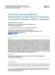
FIG. 2 Schematic of the Flash Method

4. Summary of Test Method 4.1 A small, thin disc specimen is subjected to a highintensity short duration radiant energy pulse (Fig. 2). The energy of the pulse is absorbed on the front surface of the specimen and the resulting rear face temperature rise (thermal curve) is recorded. The thermal diffusivity value is calculated from the specimen thickness and the time required for the rear face temperature rise to reach a percentage of its maximum value (Fig. 3). When the thermal diffusivity of the specimen is to be determined over a temperature range, the measurement must be repeated at each temperature of interest. NOTE 1—This test method is described in detail in a number of publications (1, 2)3 and review articles (3, 4, 5). A summary of the theory can be found in Appendix X1.

5. Significance and Use 5.1 Thermal diffusivity is an important transient thermal property, required for such purposes such as design applications, determination of safe operating temperature, process control, and quality assurance.

3 The boldface numbers given in parentheses refer to a list of references at the end of the text.

FIG. 1 Laser Pulse Shape

FIG. 3 Characteristic Thermal Curve for the Flash Method

5.2 The flash method is used to measure values of thermal diffusivity, α, of a wide range of solid materials. It is particularly advantageous because of simple specimen geometry, small specimen size requirements, rapidity of measurement and ease of handling. 5.3 Under certain strict conditions, specific heat capacity of a homogeneous isotropic opaque solid specimen can be determined when the method is used in a quantitative fashion (see Appendix X2). 5.4 Thermal diffusivity results, together with related values of specific heat capacity (Cp) and density (ρ) values, can be used in many cases to derive thermal conductivity (λ), according to the relationship: λ 5 α Cp ρ

(1)

6. Interferences 6.1 In principle, the thermal diffusivity is obtained from the thickness of the specimen and from a characteristic time function describing the propagation of heat from the front surface of the specimen to its back surface. The sources of uncertainties in the measurement are associated with the specimen itself, the temperature measurements, the performance of the detector and of the data acquisition system, the data analysis and more specifically the finite pulse time effect, the nonuniform heating of the specimen and the heat losses (radiative and conductive). These sources of uncertainty can be considered systematic, and should be carefully considered for each experiment. Errors random in nature (noise, for example) can be best estimated by performing a large number of repeat

Copyright by ASTM Int'l (all rights reserved); Mon Apr 4 05:10:23 EDT 2016 2 Downloaded/printed by Huazhong Uni of Science (Huazhong Uni of Science ) pursuant to License Agreement. No further reproductions authorized.

E1461 − 13 experiments. The relative standard deviation of the obtained results is a good representation of the random component of the uncertainty associated with the measurement. Guidelines in performing a rigorous evaluation of these factors are given in (6).

7.5 Data Recording: 7.5.1 The data acquisition system must be of an adequate speed to ensure that resolution in determining half-rise time on the thermal curve is no more than 1 % of the half-rise time, for the fastest thermal curve for which the system is qualified.

7. Apparatus The essential components of the apparatus are shown in Fig. 4. These are the flash source, specimen holder, environmental enclosure (optional), temperature detector and recording device.

7.6 Measurement of specimen’s temperature is performed using calibrated temperature sensors such as a thermocouple, optical pyrometer, platinum resistance temperature detector (RTD), etc. The temperature sensor shall be in intimate contact with or trained on the sample holder, in close proximity of the specimen.

7.1 The flash source may be a pulse laser, a flash lamp, or other device capable to generate a short duration pulse of substantial energy. The duration of the pulse should be less than 2 % of the time required for the rear face temperature rise to reach one half of its maximum value (see Fig. 3). NOTE 2—A pulse length correction may be applied (7, 8, 9) permitting use of pulse durations greater than 0.5 %.

7.1.1 The energy of the pulse hitting the specimen’s surface must be spatially uniform in intensity. 7.2 An environmental control chamber is required for measurements above and below room temperature. 7.3 The temperature detector can be a thermocouple, infrared detector, optical pyrometer, or any other sensor that can provide a linear electrical output proportional to a small temperature rise. It shall be capable of detecting 0.05 K change above the specimen’s initial temperature. The detector and its associated amplifier must have a response time not more than 2 % of the half-rise time value. 7.4 The signal conditioner includes the electronic circuit to bias out the ambient temperature reading, spike filters, amplifiers, and analog-to-digital converters.

NOTE 3—Touching the specimen with thermocouples is not recommended. Embedding thermocouples into the specimen is not acceptable.

7.7 The temperature controller and/or programmer are to bring the specimen to the temperatures of interest. 8. Test Specimen 8.1 The usual specimen is a thin circular disc with a front surface area less than that of the energy beam. Typically, specimens are 10 to 12.5 mm in diamete (in special cases, as small as 6 mm diameter and as large as 30 mm diameter have been reported as used successfully). The optimum thickness depends upon the magnitude of the estimated thermal diffusivity, and should be chosen so that the time to reach half of the maximum temperature falls within the 10 to 1000 ms range. Thinner specimens are desired at higher temperatures to minimize heat loss corrections; however, specimens should always be thick enough to be representative of the test material. Typically, thicknesses are in the 1 to 6 mm range. 8.2 Specimens must be prepared with faces flat and parallel within 0.5 % of their thickness, in order to keep the error in thermal diffusivity due to the measured average thickness, to less than 1 %. Non-uniformity of either surface (craters, scratches, markings) should be avoided 8.3 Specimen Surface Preparation—It is a good practice to apply a very thin, uniform graphite or other high emissivity coating on both faces of the specimen to be tested, prior to performing the measurements. The coating may be applied by spraying, painting, sputtering, etc. This will improve the capability of the specimen to absorb the energy applied, especially in case of highly reflective materials. For transparent materials, a layer of gold, silver, or other opaque materials must be deposited first, followed by graphite coating. For some opaque reflective materials, grit blasting of the surface can provide sufficient pulse absorption and emissivity, especially at higher temperatures, where coatings may not be stable or may react with the material. 9. Calibration and Verification

FIG. 4 Block Diagram of a Flash System

9.1 It is important to periodically verify the performance of a device and to establish the extent these errors may affect the data generated. This can be accomplished by testing one or several materials whose thermal diffusivity is well known (see Appendix X3). 9.1.1 The use of reference materials to establish validity of the data on unknown materials can lead to unwarranted statements on accuracy. The use of references is only valid

Copyright by ASTM Int'l (all rights reserved); Mon Apr 4 05:10:23 EDT 2016 3 Downloaded/printed by Huazhong Uni of Science (Huazhong Uni of Science ) pursuant to License Agreement. No further reproductions authorized.

E1461 − 13 when the properties of the reference (including half-rise times and thermal diffusivity values) are similar to those of the unknown and the temperature-rise curves are determined in an identical manner for the reference and unknown. 9.1.2 An important check of the validity of data (in addition to the comparison of the rise curve with the theoretical model), when corrections have been applied, is to vary the specimen thickness. Since the half times vary as L2, decreasing the specimen thickness by one-half should decrease the half time to one-fourth of its original value. Thus, if one obtains the same thermal diffusivity value (appropriate heat loss corrections being applied) with representative specimens from the same material of significantly different thicknesses, the results can be assumed valid. 10. Procedure 10.1 For commercially produced systems, follow manufacturer’s instructions. 10.2 The testing procedure must contain the following functions: 10.2.1 Determine and record the specimen thickness. 10.2.2 Mount the specimen in its holder. 10.2.3 Establish vacuum or inert gas environment in the chamber if necessary. 10.2.4 Determine specimen temperature unless the system will do it automatically. 10.2.5 Especially at low temperatures, use the lowest level of power for the energy pulse able to generate a measurable temperature rise, in order to ensure that the detector functions within its linear range. 10.2.6 After the pulse delivery, monitor the raw or processed thermal curve to establish in-range performance. In case of multiple specimen testing, it is advisable (for time economy) to sequentially test specimens at the same temperature (including replicate tests) before proceeding to the next test temperature. 10.2.7 The temperature stability (base line) prior and during a test shall be verified either manually or automatically to be less than 4 % of the maximum temperature rise. NOTE 4—Testing during the temperature program is not recommended as it results in lower precision.

10.2.8 Determine the specimen ambient temperature and collect the base line, transient-rise and cooling data, and analyze the results according to Section 11. 10.2.9 Change or program the specimen temperature as desired and repeat the data collection process to obtain measurements at each temperature. 10.2.10 If required, repeat the measurements at each temperature on the specimen’s cooling or on its re-heating over the same cycle. 11. Calculation 11.1 Determine the baseline and maximum rise to give the temperature difference, ∆Tmax. Determine the time required from the initiation of the pulse for the rear face temperature to reach half ∆Tmax. This is the half-rise time, t1/2. Calculate the thermal diffusivity, α, from the specimen thickness, L, and the half-rise time t1/2, as follows (1):

α 5 0.13879 L 2 /t ½

(2)

Check the validity of the experiment by calculating α at a minimum of two other points on the rise curve. The equation is as follows: α 5 k x L 2 /t x

(3)

where: tx = the time required for the temperature rise to reach x percent of ∆Tmax. Values of kx are given in Table 1. 11.1.1 Ideally, the calculated values of α for different values of x should all be the same. If the values at 25, 50 and 75 % ∆Tmax lie within 62 %, the overall accuracy is probably within 65 % at the half-rise time. If the α values lie outside of this range, the response curve should be analyzed further to see if thermal radiation heat loss, finite-pulse time or non-uniform heating effects are present. 11.1.2 Thermal radiation heat loss effects are most readily determined from the temperature of the specimen and the rear-face temperature response after 4t1/2 by plotting the experimental values of ∆T/∆Tmax versus t/t1/2 along with the values for the theoretical model. Some numbers for the theoretical model are given in Table 2. 11.1.3 Prepare a display of the normalized experimental data and the theoretical model using the tabulated values of ∆T/∆Tmax and t/t1/2 and the corresponding experimental data at several percent levels of the rise. All normalized experimental curves must pass through ∆T/∆Tmax = 0.5 and t/t1/2 = 1.0. Calculations including the 25 to 35 % and 65 to 80 % ranges are required to compare the experimental data with the theoretical curve. 11.1.4 Examples of the normalized plots for experiments that approximate the ideal case, in which both radiation heat losses and finite pulse time effect exist, are shown in Figs. 5 and 6, and Fig. 7. Various procedures for correcting for these effects are also given in Refs. (4, 7-13) and specific examples are given in 11.2 and 11.3. 11.1.5 The corrections can be minimized by the proper selection of specimen thickness. The finite pulse time effect decreases as the thickness is increased, while heat losses decrease as the thickness is reduced. 11.1.6 Non-uniform heating effects also cause deviations of the reduced experimental curve from the model because of two-dimensional heat flow. Since there are a variety of nonuniform heating cases, there are a variety of deviations. Hot center cases approximate the radiation heat loss example. Cold center cases result in the rear face temperature continuing to rise significantly after 4t1/2. Non-uniform heating may arise from the nature of the energy pulse or by non-uniform TABLE 1 Values of the Constant kx for Various Percent Rises x(%) 10 20 25 30 33.33 40 50

kx 0.066108 0.084251 0.092725 0.101213 0.106976 0.118960 ...

Copyright by ASTM Int'l (all rights reserved); Mon Apr 4 05:10:23 EDT 2016 4 Downloaded/printed by Huazhong Uni of Science (Huazhong Uni of Science ) pursuant to License Agreement. No further reproductions authorized.

x(%) 60 66.67 70 75 80 90 ...

kx 0.162236 0.181067 0.191874 0.210493 0.233200 0.303520 ...

E1461 − 13 TABLE 2 Values of Normalized Temperature Versus Time for Theoretical Model ∆ T/∆Tmax 0 0.0117 0.1248 0.1814 0.2409 0.3006 0.3587 0.4140 0.4660 0.5000 0.5587 0.5995 0.6369 0.6709 0.7019 0.7300

t/t

⁄

12

0 0.2920 0.5110 0.5840 0.6570 0.7300 0.8030 0.8760 0.9490 1.0000 1.0951 1.1681 1.2411 1.3141 1.3871 1.4601

∆ T/∆Tmax 0.7555 0.7787 0.7997 0.8187 0.8359 0.8515 0.8656 0.8900 0.9099 0.9262 0.9454 0.9669 0.9865 0.9950 0.9982 ...

t/t

⁄

12

1.5331 1.6061 1.6791 1.7521 1.8251 1.8981 1.9711 2.1171 2.2631 2.4091 2.6281 2.9931 3.6502 4.3802 5.1102 ...

FIG. 7 Normalized Rear Face Temperature Rise: Comparison of Mathematical Model (No Heat Loss) to Experimental Values with Radiation Heat Losses

For this to be valid, the evolution of the pulse intensity must be representable by a triangle of duration τ and time to maximum intensity of βτ as shown in Fig. 1. The pulse shape for the laser may be determined using an optical detector. From the pulse shape so determined, β and τ are obtained. Values of the two constants K1 and K2 for various values of β are given in Table 3 for correcting αx.

FIG. 5 Comparison of Non-dimensionalized Temperature Response Curve to Mathematical Model

11.3 Heat loss corrections can be performed using procedures proposed in a (12, 13), for example. Both of these corrections are affected by non-uniform heating effects. Corrections given in (12) by Cowan are affected by conduction heat losses to the holders in addition to the radiation heat losses from the specimen surfaces. Thus, the errors in the correction procedures are affected by different physical phenomena and a comparison of thermal diffusivity values corrected by the two procedures is useful in determining the presence or absence of these phenomena. 11.3.1 Determine the ratio of the net rise time values at times that are five and ten times the experimental half-rise time value to the net rise at the half-rise time value (12). These ratios are designated as ∆t5 and ∆t10. If there are no heat losses ∆t5 = ∆t10 = 2.0. The correction factors (KC ) for the five and ten half-rise time cases are calculated from the polynomial fits: K C 5 A1B ~ ∆t ! 1C ~ ∆t ! 2 1D ~ ∆t ! 3 1E ~ ∆t ! 4

(5)

1F ~ ∆t ! 5 1G ~ ∆t ! 6 1H ~ ∆t ! 7

FIG. 6 Normalized Rear Face Temperature Rise: Comparison of Mathematical Model (No Finite Pulse Time Effect) to Experimental Values with Finite Pulse Time

absorption on the front surface of the specimen. The former case must be eliminated by altering the energy source, while the latter may be eliminated by adding an absorbing layer and using two-layer mathematics (4, 14). 11.2 Finite pulse time effects usually can be corrected for using the equation: α 5 K 1 L 2/ ~ K 2 t x 2 τ !

where: values for the coefficients A through H are given in Table 4. Corrected values for thermal diffusivity are calculated from the following relation: α corrected 5 α

0.5

K C /0.13885

(6)

TABLE 3 Finite Pulse Time Factors β

K1

K2

0.15 0.28 0.29 0.30 0.50

0.34844 0.31550 0.31110 0.30648 0.27057

2.5106 2.2730 2.2454 2.2375 1.9496

(4)

Copyright by ASTM Int'l (all rights reserved); Mon Apr 4 05:10:23 EDT 2016 5 Downloaded/printed by Huazhong Uni of Science (Huazhong Uni of Science ) pursuant to License Agreement. No further reproductions authorized.

E1461 − 13 TABLE 4 Coefficients for Cowan Corrections Coefficients A B C D E F G H

Five Half Times

12.2.1 Statement that the response time of the detector, including the associated electronics was adequately checked, and the method used; 12.2.2 Energy pulse source; 12.2.3 Beam uniformity; 12.2.4 Type of temperature detector; 12.2.5 Manufacturer and model of the instrument used; 12.2.6 Dated version of this test method used.

Ten Half Times

−0.1037162 1.239040 −3.974433 6.888738 −6.804883 3.856663 −1.167799 0.1465332

0.054825246 0.16697761 −0.28603437 0.28356337 −0.13403286 0.024077586 0.0 0.0

where: α0.5 = the uncorrected thermal diffusivity value calculated using the experimental half-rise time. 11.3.2 Heat loss corrections based on the procedure given in Clark and Taylor (12) also use ratio techniques. For the t0.75/t0.25 ratio, that is, the time to reach 75 % of the maximum divided by the time to reach 25 % of the maximum, the ideal value is 2.272. Determine this ratio from the experimental data. Then calculate the correction factor (KR) from the following equation: K R 5 20.346146710.361578 ~ t 0.75/t 0.25! 20.06520543 ~ t

(7)

/t 0.25 ! 2

0.75

The corrected value for the thermal diffusivity at the half-rise time is αcorrected = α0.5 KR /0.13885. Corrections based on many other ratios can also be used. 11.4 If the measurements are performed at temperatures different from that where the specimen thickness has been determined, consider the presence of the linear thermal expansion effects. If these effects are not negligible, calculate the specimen thickness at each temperature and apply the usual procedure as described above. 11.5 Other parameter estimation methods may also be used, provided detailed reference to the source is reported with the data. 12. Report 12.1 The report shall contain: 12.1.1 Identification of the specimen (material) and previous history; 12.1.2 Specimen thickness, m; 12.1.3 Temperature, °C; 12.1.4 Calculated value of thermal diffusivity at x = 50 %, at the reported temperature; 12.1.5 Calculated values near x = 25 and 75 % as well as x = 50 %, or a comparison of the reduced experimental curve to the model, at each temperature; 12.1.6 Repeatability of results at each temperature; 12.1.7 Whether or not the data was corrected for thermal expansion. If this correction was made, the thermal expansion values used must be reported; 12.1.8 Description of any correction procedures for heat loss and finite pulse length effect. 12.1.9 Environmental surroundings of the specimen (gas type, pressure, etc.). 12.2 Additionally, it is beneficial to report:

13. Precision and Bias 13.1 The precision and bias information for this standard are obtained from literature meta-analysis performed in 2013. The results of study are on file at ASTM Headquarters.4 13.2 Precision: 13.2.1 Within laboratory variability may be described using the repeatability value (r) obtained by multiplying the repeatability standard deviation by 2.8. The repeatability value estimates the 95 % confidence limit. That is, two results from the same laboratory should be considered suspect (at the 95 % confidence level) if they differ by more than the repeatability value. 13.2.1.1 The within laboratory repeatability relative standard deviation from results obtained at 673 and 870 K is 2.0 %. 13.2.1.2 The within laboratory repeatability relative standard deviation is reported in the literature to be temperature dependent and to decrease with increasing temperature (15). 13.2.2 Between laboratory variability may be described using the reproducibility value (R) obtained by multiplying the reproducibility standard deviation by 2.8. The reproducibility value estimates the 95 % confidence limit. That is, results obtained in two different laboratories should be considered suspect (at the 95 % confidence level) if they differ by more than the reproducibility value. 13.2.2.1 The between laboratory reproducibility standard deviation from results obtained at 673 K is 13 % and at 870 K is 8.1 %. 13.2.2.2 The between laboratory reproducibility standard deviation is observed to be temperature dependent and to decrease with increasing temperature (15). 13.3 Bias: 13.3.1 Bias is the difference between the mean value obtained and an accepteble reference value for the same material. 13.3.2 The mean value for the thermal diffusivity for AXM-5Q graphite was found to be 0.259 cm2/s at 673 K and 0.208 cm2/s at 870 K. The best estimate literature value for AXM-5Q graphite at these temperatures are 0.279 and 0.208 cm2/s, respectively representing -7.7 % and 0 % bias at these temperatures. 13.3.3 Bias is observed to be temperature dependent and to decrease with increasing temperature (15).

4 Supporting data have been filed at ASTM International Headquarters and may be obtained by requesting Research Report RR:E37-1043. Contact ASTM Customer Service at [email protected].

Copyright by ASTM Int'l (all rights reserved); Mon Apr 4 05:10:23 EDT 2016 6 Downloaded/printed by Huazhong Uni of Science (Huazhong Uni of Science ) pursuant to License Agreement. No further reproductions authorized.

E1461 − 13 14. Keywords 14.1 flash method; infrared detectors; intrinsic thermocouples; specific heat capacity; thermal conductivity; thermal diffusivity; transient temperature measurements

APPENDIXES X1. THEORY

X1.1 The Ideal Case—The physical model of the pulse method is founded on the thermal behavior of an adiabatic (insulated) slab of material, initially at constant temperature, whose one side has been subjected to a short pulse of energy. The model assumes: • one dimensional heat flow; • no heat losses from the slab’s surfaces; • uniform pulse absorption at the front surface; • infinitesimally short pulse duration; • absorption of the pulse energy in a very thin layer; • homogeneity and isotropy of the slab material; • property invariance with temperature within experimental conditions. In deriving the mathematical expression from which the thermal diffusivity is calculated, Parker (1) starts from the equation of the temperature distribution within a thermally insulated solid of uniform thickness L, as given by Carslaw and Jaeger (16): 1 T ~ x,t ! 5 L 1

At the rear surface, where x = L, the temperature history can be expressed by: T ~ L,t ! 5

F

S

` Q 2n 2 π 2 112 ~ 21 ! n ·exp αt ρCL L n51

(

V ~ L,t ! 5 ω5

T ~ L,t ! TM

π 2 αt L2

( ~ 21 ! ·exp~ 2n n

D

* T ~ x,0 ! cos n Lπx dx L

0

(X1.1)

where α is the thermal diffusivity of the material. If a pulse of radiant energy Q is instantaneously and uniformly absorbed in the small depth g at the front surface x = 0, the temperature distribution at that instant is given by Q ρ·C·g

(X1.2)

for 0 < x < g and T ~ x,0 ! 5 0 (X1.3) for g < x < L. With this initial condition, Eq X1.1 can be written as:

(

n πg 2n 2 π 2 L αt ·exp n πg L2 L

sin

S

D

4

(X1.4)

where ρ is the density and C is the specific heat capacity of the material. In this application only a few terms will be needed, and since g is a very small number for opaque materials, sin

ω!

(X1.9)

When V = 0.5, ω = 1.38, and therefore: α5

1.38·L 2 π 2t 1

(X1.10)

2

or: L2 t1

(X1.11)

2

n πx 2n 2 π 2 αt 2 ` exp · cos L n51 L2 L

3

2

n51

α 5 0.1388

` n πx Q 112 cos T ~ x,0 ! 5 ρCL L n51

(X1.8)

`

V 5 112

0

T ~ x,0 ! 5

(X1.7)

TM represents the maximum temperature at the rear surface. The combination of Eq X1.6-X1.8 yields:

* T ~ x,0 ! dx

S

(X1.6)

Two dimensionless parameters, V and ω can be defined:

L

(

DG

n πg n πg ' L L

(X1.5)

where t ⁄ is the time required for the back surface to reach half of the maximum temperature rise. A pulse experiment is schematicallyis represented in Fig. 2. As a result, a characteristic thermal curve of the rear face is created (Fig. 3). 12

X1.2 The Non-Ideal Case—The inadequacy of the Parker solution became obvious almost immediately after its introduction, as nearly every one of these assumptions is violated to some extent during an experiment. So, gradually, investigators introduced various theories to describe the real process, and solutions describing corrections to counter the violation of each of the boundary conditions. The ideal correction would encompass all factors present, but to date, no such general correction has been developed. Instead, individual or paired corrections accounting for deviations were introduced. The result is that one may end up with an array of numbers that vary substantially after using these corrections. This is understandable, as historically, each investigator has focused on one or another deviation from the ideal model, while assuming ideality and constancy of the others. This by itself is a substantial violation of principles, as in reality all parameters vary concurrently, in an extent dictated by the particular conditions of the experiment. Some situations may aggravate one condition, for example having a long pulse, others may introduce other deviations, such as excessive heat losses from the front face due to using very powerful pulses,

Copyright by ASTM Int'l (all rights reserved); Mon Apr 4 05:10:23 EDT 2016 7 Downloaded/printed by Huazhong Uni of Science (Huazhong Uni of Science ) pursuant to License Agreement. No further reproductions authorized.

E1461 − 13 etc. It is therefore incumbent to choose the most proper correction in harmony with the conditions of the experiment analyzed. The finite pulse width effect, for example, occurs strongly when thin specimens of high thermal diffusivity are tested (2, 8, 9, 17, 18), while the radiative heat losses become dominant at high temperatures (12), when testing thick specimens. In contrast, nonuniform heating can occur during any thermal diffusivity experiment (19). This can occur when a circular surface smaller than the specimen itself is irradiated, or the flux density of the pulse varies from point-to-point over the specimen’s surface. For the same amount of absorbed energy, the dimensionless half-max time of the resulting thermal curve at the center of the rear face of the specimen differs consider-

ably from the one obtained with uniform irradiation. This effect can be reduced by increasing the ratio between the specimen’s thickness and its radius. The same result can be achieved by using a temperature measurement system, which automatically integrates the signal obtained from the rear face of the specimen. It is a very difficult task to choose the best correction, and often not enough information is known about the equipment and the testing parameters to do it prudently. In principle, one must return to the original premise: the accuracy of the data depends on the agreement between the mathematical and experimental models. The purpose of applying corrections to the experimental data is to bring it to closer agreement with the ideal solution by accounting for the aberrations.

X2. MEASUREMENT OF SPECIFIC HEAT CAPACITY AND CALCULATION OF THERMAL CONDUCTIVITY

X2.1 The fundamental relationship between thermal diffusivity (α), thermal conductivity (λ), specific heat capacity (Cp), and density (ρ), α5

λ C p ·ρ

(X2.1)

allows the calculation of thermal conductivity, a much sought after property, with the knowledge of the other properties. A method was developed (1) where the specific heat capacity of a specimen is determined when the thermal diffusivity test is performed in a quantitative fashion. Caution shall be used in performing this extenstion as errors abounds. In the course of an ordinary thermal diffusivity test, the amount of energy is important only to the extent that it will generate a sufficient rear face signal. For operating in a calorimetric mode, the energy level must be known closely, controllable and repeatable. Approximating adiabatic conditions, the laser pulse and the detector can be calibrated in unison when a specimen of known specific heat capacity is tested. The measurement will yield thermal diffusivity, and also a relative measure of energy expressed in terms of the absolute value of the maximum attained temperature. By testing an unknown specimen after this “calibration”, the specific heat capacity can be calculated from its maximum attained temperature, relative to the one obtained for the standard. There are several conditions that must be satisfied in order for this process to be valid: X2.1.1 The energy source must be able to reproduce within 5 % the energy of a pulse based on the power defining parameter (charge voltage for lasers, for example) over a period of time. X2.1.2 The detector must maintain its sensitivity over a period of time without drift, gain change, and within a linear response range. X2.1.3 The reference specimen and the unknown specimen must be very similar in size, proportions, emissivity, and opacity, to approximate adiabatic behavior to the same extent. Both the reference and the unknown specimen should be coated with a thin uniform graphite layer, to ensure that the emissivity of the two materials is the same.

X2.1.4 Both reference and unknown specimen must be homogeneous and isotropic, as Eq X2.1 only applies for those materials. Heterogeneous and anisotropic materials will frequently produce erroneous data. The process is not purely calorimetric, since the maximum temperature rise is derived from the signal provided largely by the components with the highest thermal diffusivity, while the internal equilibration may take place after that point in time. For this reason, this method tends to give erroneous results for specific heat capacity for materials with large anisotropy (typically composites with an ordered directional structure) and for mixtures of components with greatly differing thermal diffusivities. X2.1.5 The reference and the unknown must be tested very close to each other, both temporally (preferably only minutes apart) and thermally (strictly at the same temperature, in the same environment). X2.1.6 This being a differential measurement, it is highly desirable to have both reference and unknown tested side-byside and with very small time intervals in between. It is also desirable to test standard/specimen/standard, to minimize errors from pulse energy variations. X2.2 The specimen’s density may be calculated from results of weight measurements and computed volume. It is appropriate to calculate the density at each temperature from the room temperature density, using thermal expansion data. Consult Test Method E228 for details. X2.3 Thermal conductivity may be calculated using Eq X2.1, from the measured values of thermal diffusivity, specific heat capacity and density. X2.3.1 When measured values of specific heat capacity are used, the constrains listed under X2.1.1 – X2.1.6 also apply to the resultant thermal conductivity. X2.3.2 It is permissible to use specific heat capacity and density data from other sources than the measurements above. X2.4 Reporting specific heat capacity or thermal conductivity obtained in this manner must be accompanied by:

Copyright by ASTM Int'l (all rights reserved); Mon Apr 4 05:10:23 EDT 2016 8 Downloaded/printed by Huazhong Uni of Science (Huazhong Uni of Science ) pursuant to License Agreement. No further reproductions authorized.

E1461 − 13 X2.4.1 An accuracy statement determined; X2.4.2 The time elapsed between reference and test pulses;

X2.4.3 Reference material used.

X3. REFERENCE MATERIALS

X3.1 Only a few Standard Reference Materials (SRM) are available from the National Metrology Institutes for thermal diffusivity. However, a large amount of data is available in the literature on a number of industry-accepted reference materials that have been used for verification purposes. X3.1.1 A valuable summary and data bank of thermal diffusivity values found in the literature that also provides recommended values for a wide range of materials, is also available (20).

298 to 1025 K. Its certificate lists an uncertainty of 6 6 %. The thermal diffusivity value is determined from the equation: α ~~ mm! 2 s 21 !

54.406 2 1.35 31022 T12.133 31025 T 2 2 1.541 31028 T 3 14.147 310212T 4

(X3.1)

where T is in K.

X3.2 A glass-ceramic thermal diffusivity standard reference material, BCR-724,5 is available for the temperature range of 5 The sole source of supply of BCR-724 known to the committee at this time is theInstitute for Reference Materials and Measurements, Retiesweg 11, B-2440 Geel, Belgium, [email protected]. If you are aware of alternative suppliers, please provide this information to ASTM International Headquarters. Your comments will receive careful consideration at a meeting of the responsible technical committee,1 which you may attend.

REFERENCES (1) Parker, W. J., Jenkins, R. J., Butler, C. P., and Abbott, G. L., “Flash Method of Determining Thermal Diffusivity Heat Capacity and Thermal Conductivity,” Journal of Applied Physics, Vol 32, 1961, pp. 1679–1984. (2) Watt, D. A., “Theory of Thermal Diffusivity of Pulse Technique,” British Journal of Applied Physics, Vol 17, 1966, pp. 231–240. (3) Righini, F., and Cezairliyan, A., “Pulse Method of Thermal Diffusivity Measurements, A Review,” High Temperatures—High Pressures, Vol 5, 1973, pp. 481–501. (4) Taylor, R. E., “Heat Pulse Diffusivity Measurements,” High Temperatures—High Pressures, Vol 11, 1979, pp. 43–58. (5) Taylor, R. E., “Critical Evaluation of Flash Method for Measuring Thermal Diffusivity,” Revue Internationale des Hautes Temperatures et des Refractaires, Vol 12, 1975, pp. 141–145. (6) Taylor, B. N., Kuyatt, C. E., “Guidelines for Evaluating and Expressing the Uncertainty of NIST Measurements Results,” NIST Technical Note 1297, Gaithersburg, MD, 1994. (7) Cape, J. A., and Lehman, G. W., “Temperature and Finite Pulse-Time Effects in the Flash Method for Measuring Thermal Diffusivity,” Journal of Applied Physics, Vol 34, 1963, pp. 1909–1913. (8) Taylor, R. E., and Clark, III, L. M., “Finite Pulse Time Effects in Flash Diffusivity Method,” High Temperatures—High Pressures, Vol 6, 1974, pp. 65–72. (9) Larson, K. B., and Koyama, K., “Correction for Finite Pulse-Time Effects in Very Thin Samples Using the Flash Method of Measuring Thermal Diffusivity,” Journal of Applied Physics, Vol 38, 1967, pp. 465–474. (10) Heckman, R. C., “Error Analysis of the Flash Thermal Diffusivity Technique,” Thermal Conductivity 14, Klemens, P. G., and Chu, T. K., eds. Plenum Publishing Corp., NY, 1974, pp. 491–498. (11) Sweet, J. N., “Effect of Experimental Variables on Flash Thermal Diffusivity Data Analysis,” Thermal Conductivity 20, Hasselman, D.

(12)

(13)

(14)

(15)

(16) (17)

(18)

(19)

P. H., ed., Plenum Publishing Corp., NY, 1974, p. 287. See also Sweet, J. N., “Data Analysis Methods for Flash Diffusivity Experiments,” Sandia National Laboratory Report SAND 89-0260, (Available from NTIS), February, 1989. Clark, L. M., III, and Taylor, R. E., “Radiation Loss in the Flash Method for Thermal Diffusivity,” Journal of Applied Physics, Vol 46, 1975, pp. 714–719. Cowan, R. D., “Pulse Method of Measuring Thermal Diffusivity at High Temperatures,” Journal of Applied Physics, Vol 34, 1963, pp. 926–927. Larson, K. B., and Koyama, K., “Measurement of Thermal Diffusivity, Heat Capacity and Thermal Conductivity in Two-Layer Composite Samples by the Flash Method,” in Proceedings 5th Thermal Conductivity Conference, University of Denver, Denver, CO, 1965, pp. 1-B-1 to 1-B-24. Fitzer, “Thermal Properties of Solid Materials, Project Section II – Cooperative Measurements of Heat Transport Phenomena of Solid Materials at High Temperatures,” Advisory Group for Aerospace Research and Development (AGARD), North Atlantic Treaty Organization, AGARD Report No. 606, 1973. Carslaw H. S., and Jeager, J. C., Conduction of Heat in Solids, 2nd ed., Oxford University Press, London, 1959. Taylor, R. E., and Cape, J. A., “Finite Pulse-Time Effects in the Flash Diffusivity Technique,” Applied Physics Letters, Vol 5, 1964, pp. 210–212. Azumi, T., and Takahashi, Y., “Novel Finite Pulse-Width Correction in Flash Thermal Diffusivity Measurement,” Review of Scientific Instruments, 1981, pp. 1411–1413. Mackay, J. A., and Schriempf, J. T., “Corrections for Nonuniform Surface Heating Errors in Flash-Method Thermal Diffusivity Measurements,” Journal of Applied Physics, Vol 47, 1976, pp. 1668–1671.

Copyright by ASTM Int'l (all rights reserved); Mon Apr 4 05:10:23 EDT 2016 9 Downloaded/printed by Huazhong Uni of Science (Huazhong Uni of Science ) pursuant to License Agreement. No further reproductions authorized.

E1461 − 13 (20) Touloukian, Y. S., Powell, R. W., Ho, C. Y., and Nicolaou, M., “Thermal Diffusivity,” Thermophysical Properties of Matter, Vol 10, IFI/Plenum, NY, 1973.

BIBLIOGRAPHY (1) Baba, T., Cezairliyan, A., “Thermal Diffusivity of POCO AXM-5Q1 Graphite in the Range 1500 to 2500 K Measured by a Laser-Pulse Technique,” International Journal of Thermophysics, Vol 15, No. 2, 1994, p. 343–364. (2) Beck, J. V., and Dinwiddie, R. B., “Parameter Estimation Method for Flash Thermal Diffusivity with Two Different Heat Transfer Coefficients,” in Thermal Conductivity 23, Dinwiddie, R., Graves, R., and Wilkes, K., eds., Technomic Publishing Co., Lancaster, 1996, pp. 107–116. (3) Begej, S., Garnier, J. E., Desjarlais, A. O., and Tye, R. P.,“ Ex-Reactor Determination of Thermal Contact Conductance Between Uranium Dioxide Zircaloy-4 Interfaces,” Thermal Conductivity 16, Larsen, D. C., ed., Plenum Press, NY, 1983, pp. 221–232. (4) Begej, S., Garnier, J. E., Desjarlais, A. O., and Tye, R. P., “Determination of Thermal Gap Conductance Between Uranium Dioxide; Zicaloy-4 Interfaces,” Thermal Conductivity 16, Larsen, D. C., ed., Plenum Press, NY, 1983, pp. 211–219. (5) Cezairliyan, A., Baba, T., and Taylor, R., “A High-Temperature Laser-Pulse Thermal Diffusivity Apparatus,” International Journal of Thermophysics, Vol 15, 1994, pp. 317–364. (6) Chistyakov, V. I., “Pulse Method of Determining the Thermal Conductivity of Coatings,” Teplofiz. Vys. Tempe., Vol 11, 1976, p. 832; English Translation: High Temperatures—High Pressures, Vol 11, 1973, pp. 744–748. (7) Degiovanni, A., Gery, A., Laurent, M., and Sinicki, G., “Attaque impulsionnelle appliquee a la mesure des resistances de contact et de la diffusivite termique,” Entropie, Vol 64, 1975, p. 35. (8) Degiovanni, A., “Correction de longueur d’impulsion pour la measure de la diffusivity thermique par la methode flash,” International Journal of Heat and Mass Transfer , Vol 30, 1988 , pp. 2199–2200. (9) European Cooperation for Accreditation EA-4/02, “Expression of the Uncertainty of Measurement in Calibration,” Edition 1, April 1997. (10) Goldner, F., Thesis, “A Microtransient Technique for the Determination of Fluid Thermal Diffusivities,” The Catholic University of America, Washington, DC, No. 70-22, p. 142. (11) Hasselman, D. P. H., and Donaldson, K. Y., “Effects of Detector Nonlinearity and Specimen Size on the Apparent Thermal Diffusivity of NIST 8425 Graphite,” International Journal of Thermophysics, Vol 11, 1990, pp. 573–585. (12) Heckman, R. C., “Intrinsic Thermocouples in Thermal Diffusivity Experiments,” Proceedings Seventh Symposium on Thermophysical Properties, Cezairliyan, A., ed., ASME, NY, 1977, pp. 155–159. (13) Heckman, R. C., “Error Analysis of the Flash Thermal Diffusivity Technique,” in Proceedings 14th International Thermal Conductivity Conference, Plenum Press, New York, 1976. (14) Henning, C. D., and Parker, R., “Transient Response of an Intrinsic Thermocouple,” Journal of Heat Transfer, Transactions of ASME, Vol 89, 1967, pp. 146–152. (15) ISO Guide to the Expression of Uncertainty in Measurement.

(16) Koski, J. A., “Improved Data Reduction Method for Laser Pulse Diffusivity Determination with the Use of Minicomputers,” in Proceedings of the 8th Symposium on Thermophysical Properties, 2, The American Society of Mechanical Engineers, p. 94, New York, 1981. (17) Lee, H. J., and Taylor, R. E., “Determination of Thermophysical Properties of Layered Composites by Flash Method,” Thermal Conductivity 14, Klemens, P. G., and Chu, T. K., eds. Plenum Publishing Corp., NY, 1974, pp. 423 –434. (18) Lee, T. Y. R., and Taylor, R. E., “Thermal Diffusivity of Dispersed Materials,” Journal of Heat Transfer, Vol 100, 1978 , pp. 720–724. (19) Minges, M., “Analysis of Thermal and Electrical Energy Transport in POCO AXM-5Q1 Graphite,” International Journal of Heat and Mass Transfer, Vol 20, 1977, pp. 1161–1172. (20) “Standard Reference Materials: A Fine-Grained, Isotropic Graphite for Use as NBS Thermophysical Property RM’s from 5 to 2500 K,” NBS Special Publication 260-89, Gaithersburg, 1984. (21) Stroe, D. E., Gaal, P. S., Thermitus, M. A., and Apostolescu, A. M., “A Comparison of Measurement Uncertainities for Xenon Discharge Lamp and Laser Flash Thermal Diffusivity Instruments:, in Proceedings of the 27th International Thermal Conductivity Conference, Wang, H., and Porter, W., eds., DE Stech Publications, Inc., Lancaster, 2005, pp. 473–483. (22) Suliyanti, M. M., Baba, T., and Ono, A., “Thermal Diffusivity Measurements of Pyroceram 9606 by Laser Flash Method,” in Thermal Conductivity 22, Tong, T. W., eds., Plenum Publishing Corp., NY, 1974, pp. 80–90. (23) Taylor, R. E., “Critical Evaluation of Flash Method for Measuring Thermal Diffusivity,” Report PRF-6764. Available from National Science Technical Information Service, Springfield, VA 22151, 1973. (24) Taylor, R. E., Lee, T. Y. R., and Donaldson, A. B., “Thermal Diffusivity of Layered Composites,” Thermal Conductivity 15, Mirkovich, V. V., ed., Plenum Publishing Corp., NY, 1978 , pp. 135–148. (25) Taylor, R. E., “Heat Pulse Diffusivity Measurements,” High Temperatures – High Pressures, Vol 11, 1979, pp. 43–58. (26) Taylor, R. E., and Groot, H., “Thermophysical Properties of POCO Graphite,” High Temperatures—High Pressures, Vol 12, 1980 , pp. 147–160. (27) Taylor, R. E., “Thermal Diffusivity of Composites,” High Temperatures – High Pressures, Vol 15, 1983, p. 299. (28) Taylor, R. E. and Maglic, K. D., “Pulse Method for Thermal Diffusivity Measurement,” in Compendium of Thermophysical Property Measurement Methods, Vol 1, Survey of Measurement Techniques, Plenum Press, New York and London, 1984. (29) Thermitus, M. A., and Gaal, P. S., “Specific Heat Measurement in a Multisample Environment with the Laser Flash Method,” in Proceedings of the 24th International Thermal Conductivity Conference, Gaal, P. S., and Apostolescu, D. E., eds., Technomic Publishing Co., Lancaster, 1999.

Copyright by ASTM Int'l (all rights reserved); Mon Apr 4 05:10:23 EDT 2016 10 Downloaded/printed by Huazhong Uni of Science (Huazhong Uni of Science ) pursuant to License Agreement. No further reproductions authorized.

E1461 − 13 (30) Thermitus , M. A., and Gaal, P. S., “Specific Heat Capacity of Some Selected Materials with the Laser Flash Method,” in Proceedings of the 25th International Thermal Conductivity Conference, Uher, C., and Morelli, D., eds., Technomic Publishing Co., Lancaster, 2000, p. 340. (31) Tye, R. P., ed., Thermal Conductivity 1, Academic Press, London and New York, 1969.

(32) Wang, H., Dinwiddie R. B., and Gaal, P. S., “Multiple Station Thermal Diffusivity Instrument,” in Thermal Conductivity 23, Dinwiddie, R., Graves, R., and Wilkes, K., eds., Technomic Publishing Co., Lancaster, 1996, pp. 119–123.

ASTM International takes no position respecting the validity of any patent rights asserted in connection with any item mentioned in this standard. Users of this standard are expressly advised that determination of the validity of any such patent rights, and the risk of infringement of such rights, are entirely their own responsibility. This standard is subject to revision at any time by the responsible technical committee and must be reviewed every five years and if not revised, either reapproved or withdrawn. Your comments are invited either for revision of this standard or for additional standards and should be addressed to ASTM International Headquarters. Your comments will receive careful consideration at a meeting of the responsible technical committee, which you may attend. If you feel that your comments have not received a fair hearing you should make your views known to the ASTM Committee on Standards, at the address shown below. This standard is copyrighted by ASTM International, 100 Barr Harbor Drive, PO Box C700, West Conshohocken, PA 19428-2959, United States. Individual reprints (single or multiple copies) of this standard may be obtained by contacting ASTM at the above address or at 610-832-9585 (phone), 610-832-9555 (fax), or [email protected] (e-mail); or through the ASTM website (www.astm.org). Permission rights to photocopy the standard may also be secured from the Copyright Clearance Center, 222 Rosewood Drive, Danvers, MA 01923, Tel: (978) 646-2600; http://www.copyright.com/

Copyright by ASTM Int'l (all rights reserved); Mon Apr 4 05:10:23 EDT 2016 11 Downloaded/printed by Huazhong Uni of Science (Huazhong Uni of Science ) pursuant to License Agreement. No further reproductions authorized.