Feb 15, 2013 - Université Pierre et Marie Curie - Paris 6, Laboratoire de Physique Théorique de la Mati`ere Condensée,. 4, Place Jussieu, Tour 12, 5`eme ...
Thermal phase transitions in Artificial Spin-Ice Demian Levis,1 Leticia F. Cugliandolo,1 Laura Foini,1 and Marco Tarzia2 1
arXiv:1302.3725v1 [cond-mat.stat-mech] 15 Feb 2013
Universit´e Pierre et Marie Curie - Paris 6, Laboratoire de Physique Th´eorique et Hautes Energies, 4, Place Jussieu, Tour 13, 5`eme e´ tage, 75252 Paris Cedex 05, France 2 Universit´e Pierre et Marie Curie - Paris 6, Laboratoire de Physique Th´eorique de la Mati`ere Condens´ee, 4, Place Jussieu, Tour 12, 5`eme e´ tage, 75252 Paris Cedex 05, France We use the sixteen vertex model to describe bi-dimensional artificial spin ice (ASI). We find excellent agreement between vertex densities in fifteen differently grown samples and the predictions of the model. Our results demonstrate that the samples are in usual thermal equilibrium away from a critical point separating a disordered and an anti-ferromagnetic phase in the model. The second-order phase transition that we predict suggests that the spatial arrangement of vertices in near-critical ASI should be studied in more detail in order to verify whether they show the expected space and time long-range correlations. PACS numbers: 75.50.Lk, 75.10.Hk, 05.70.Jk, 05.70.Ln
Hard local constraints produce a rich variety of collective behavior such as the splitting of phase space into different topological sectors and the existence of “topological phases” that cannot be described with conventional order parameters [1]. In geometrically constrained magnets, the local minimization of the interaction energy on a frustrated unit gives rise to a macroscopic degeneracy of the ground state [2], unconventional phase transitions [3, 4], the emergence of a “Coulomb” phase with long-range correlations [5, 6] and slow dynamics [7, 8] in both 2D and 3D systems. In this work we focus on a paradigm with these features: spin-ice, a class of magnets frustrated by the ice-rules [9–11]. In natural spin-ice the ice rules are due to two facts: the pyrochlore lattice structure, in which rare earth magnetic ions sit on the vertices of corner sharing tetrahedra, and the ferromagnetic interaction between the Ising-like moments that are forced to lie on the edges joining the centers of neighboring tetrahedra by crystal fields. The energy of each unit cell is thus minimized by configurations with two spins pointing in and two out of the center of the cell. All configurations satisfying the local constraint are degenerate ground states if the ice-rule preserving vertices are equally probable. This is the same mechanism whereby water ice has a non-vanishing zeropoint entropy that is, indeed, remarkably close to the one of the Dy2 Ti2 O7 spin-ice compound [12]. These materials received a renewed interest in recent years when a formal mapping to magnetostatics suggested to interpret the local configurations violating the spin-ice rule as magnetic charges [13]. However, the detailed study of such defects in 3D remains a hard experimental task. Bi-dimensional Ising-like ice-models had no experimental counterpart until recently when it became possible to manufacture artificial samples made of arrays of elongated singledomain ferromagnetic nano-islands frustrated by dipolar interactions. The beauty of artificial spin-ice (ASI) is that the interaction parameters can be precisely engineered—by tuning the distance between islands, i.e. the lattice constant, or by applying external fields—and the microstates can be directly imaged with magnetic force microscopy (MFM) [14]. These systems should set into different phases depending on the ex-
� �
��
a=ω1 =ω2
�
�
��
b=ω3 =ω4
�
� ��
��
c=ω5 =ω6
e=ω9 =ω10 =...=ω16
�
�
��
d=ω7 =ω8
� �
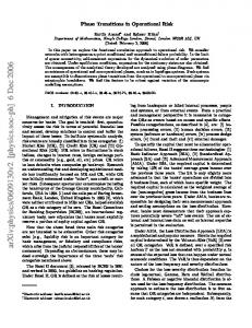
Figure 1. Sixteen vertex configurations and their statistical weights ωi ∝ exp (−β�i ). The first six-vertices, v1 , . . . v6 , verify the icerule and have vanishing magnetic charge. Vertices v1 , . . . , v4 carry a dipolar moment while v5 and v6 do not. The last ten vertices are “defects”: v7 and v8 have magnetic charge ±4 and no dipole moment while v9 , . . . , v16 have magnetic charge ±2 and a net dipole moment.
perimental conditions [15]. However, the lack of thermal fluctuations due to the high energy barriers for single spin-flips, had prevented the observation of the expected two-fold degenerate antiferromagnetic (AF) ground state. Recently, these problems have been partially overcome via (i) the gradual magneto-fluidization of an initially polarized state [16] and (ii) the thermalization of the system during the slow growth of the samples [17]. Although with de-magnetization the actual AF state of square ASI was never reached, the statistical study of a large number of frozen configurations of samples with up to 106 vertices at interaction-dominated low energies became possible [16]. With the procedure proposed in (ii) large regions with AF order were formed in a few samples when suf1 ficiently small lattice constant and weak disorder were used. Whether the sampling of a conventional thermal equilibrium ensemble is achieved in this way is a question that was raised in [17, 18] and that we will address here. The purpose of this letter is to interpret and explain very recent experimental observations on ASI [16–18]. With this aim we consider a simple schematic model for 2D dipolar spinice, the sixteen-vertex model (see Fig. 1) [4, 8], where dipolar interactions beyond nearest-neighbor vertices are neglected. We compare the equilibrium and out-of-equilibrium properties of the model with the experimental results and we match the behavior of several observables (such as the densities of
2 1
(a)
(b)
(c)
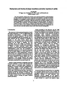
Figure 2. (Color online.) Characteristic configurations of the ground state (d = e = 0) of three different phases of the sixteen-vertex model on the square lattice. (a) Antiferromagnetic (c-AF) order. Reversing the central (red) loop yields an elementary excitation. (b) Collective spin liquid (SL) phase. (c) Frozen ferromagnetic (FM) order. The reversed vertical string (red line) is an extended excitation.
different vertex types hni i) with data on ASI samples [17, 18]. This approach is at face value similar but actually very different from the one used in previous studies [16, 18], where data were fitted in terms of single independent vertices (with no topological interactions), as hni i ∝ exp(−βeff �i ), with the effective temperature βeff introduced as a fitting parameter. On the contrary, in our approach frustrated interactions are fully taken into account. This analysis allows us to address the issue of thermalization of ASI samples and to make several predictions that could be tested in the lab. The samples and the model. In their simplest setting ASI are 2D arrays of elongated single-domain permalloy islands whose shape anisotropy defines Ising-like spins arranged along the edges of a regular square lattice. Spins interact through dipolar exchanges and the dominant contributions are the ones between neighboring islands across a given vertex. The sample is frustrated since no configuration of the surrounding spins can minimize all pair-wise dipole-dipole interactions on a vertex. In samples with no height offset (h = 0) 2D square symmetry defines four relevant vertex types of increasing energy, where the c vertices (see Fig. 1) take the lowest value, leading to a ground state with staggered c-AF order [see Fig. 2(a)]. Note that the relative energies of the different vertex configurations could be tuned by h in such a way that the ground state displayed FM order [see Fig. 2(c)] [15]. We mimic the experimental samples with the sixteen-vertex model defined as follows: Ising spins sit along the edges of an L × L square lattice. Long-range interactions beyond next nearest neighbor spins are neglected and the energies of the sixteen vertex configurations are attributed as explained above. The total energy is given terms of populations, ni , Pin 16 of distinct vertex types, E = i=1 ni �i , each with a given magnetostatic energy �i . Note that, despite the simple form of E, nontrivial frustrated topological interactions between vertices are present, due to the fact that each pair of neighboring vertices shares the spin sitting along the edge joining them. The model is coupled to a thermal bath at inverse temperature β. We introduce the statistical weights ωi ∝ exp(−β�i ), that in the literature of vertex models are usually referred as a = ω1 = ω2 , b = ω3 = ω4 , c = ω5 = ω6 , d = ω7 = ω8 and e = ω9 = . . . = ω16 [4] (see Fig. 1). The equilibrium
< ni >
0.8 nc na,b ne nd
0.6 0.4 0.2 0 0
0.5
1
1.5
2
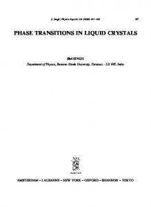
βǫ0 Figure 3. (Color online.) Average densities of different vertex types as a function of β�0 . Full symbols with error bars are experimental data [18], hni iexp . Empty symbols with dotted lines correspond to the equilibrium CTMC data, hni isim . The CVBP analytic solution, hni iM F , of the sixteen-vertex model is shown in solid lines.
properties of the model can thus be described in terms of four different statistical weights satisfying c > (a = b) > e > d. We study the equilibrium and out-of-equilibrium properties of the sixteen-vertex model in two ways. We perform numerical simulations of the 2D model with a Monte-Carlo algorithm with single-spin updates improved with the rejectionfree Continuous Time set-up (CTMC). We also employ an analytic approach put forward in [19], based on a sophisticated version of a cluster variational mean-field Bethe-Peierls (CVBP) formalism, by defining the model on a coordinationfour tree made of square plaquettes (an extension over the tree of single vertices is necessary to correctly describe an AF phase populated by finite loop fluctuations, see Fig. 2). Details of the calculations have already been extensively reported in [19], where the phase diagram was derived for generic values of the ratios a/c, b/c, d/c, e/c, showing that the CVBP technique describes with extremely good accuracy the equilibrium properties as compared to MC simulations. Density of vertices. In the experiments in [17, 18] the thickness of the magnetic islands grows by deposition (at constant temperature and all other external parameters within experimental accuracy) on fifteen lattices with five different lattice constants and using three material underlayers (Si, Ti, Cr) in each of them. (We refer to the supplementary material in [18] for more details on the parameters and materials used.) The Ising spins flip by thermal fluctuations during the growth process. However, as the energy barrier for single spin flips increases with the size of the islands, once a certain thickness is reached the barrier crosses over the thermal fluctuations of the bath, kB T , and the spins freeze. At the end of the growth process, the spin configurations are imaged with MFM and the number of vertices of each kind are counted on five independent square areas with, roughly, 27 × 27 vertices each. Average values (and statistical errors) are also estimated. Our analysis is as follows. For each set of vertex concentrations measured in [18] at a given lattice constant, we de-
3 1
5
(a)
4 L = 30 40 50 60
2 (a)
(b) 1
0
0 -1
-0.5
0 (β − βc )/βc
0.5
1
-1
-0.5
0
0.5
t = 102 t = 3.102 t = 103 t = 3.103 t = 104
10−1
1
(β − βc )/βc
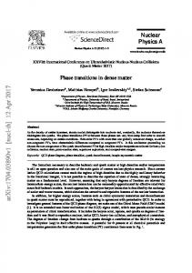
Figure 4. (Color online.) Staggered magnetization M− (a) and specific heat C (b) as a function of the distance to the inverse critical temperature βc for system sizes L = 30, 40, 50, 60. The (red) solid lines are the results of the CVBP analytic calculation.
termine the statistical weights c, a, e, and d—and thus β�c , β�a , β�e , and β�d — that better match the data, by solving the sixteen-vertex model with the CVBP approximation and imposing: P ni e−H(a,c,d,e) (1) hni iexp = hni iM F = PC −H(a,c,d,e) , Ce
where the sum runs over all possible vertex configurations C. Surprisingly enough, it turns out that the energy ratios are approximatively constant within the statistical errors for almost all the lattice spacings of the as-grown samples, and coincide with the values used by Nisoli et al. [16]. Such energy ratios can be rationalized in term of magnetostatic exchanges due to dipolar interactions between the islands of the sample associated to each vertex configuration. More precisely, each dipole is considered as a pair of oppositely charged monopoles sitting on the vertices, and only Coulomb interactions between monopoles around a single √ vertex are taken into ac2)/`, �a = −2/`, �e = 0, count, yielding: � = 2(1 − 2 c √ �d = 2(2 2 + 1)/` (` being the lattice constant). As a consequence, the statistical weights of the sixteen-vertex model can be expressed in term of a single energy scale �0 as c = 1, a = d �0 e−β�0 , e = e−βre �0 , and d = e−βr , with √ the energy ratios √ re and rd being equal to r = (2 2 − 1)/(2 2 − 2) ' 2.207 e √ √ and rd = 2 2/( 2 − 1) ' 6.828. Remarkably, no fitting parameter nor effective temperature needs to be introduced to describe the data: β is the true inverse temperature at which experiments are performed and �0 is an energy scale that only depends on the lattice constant and the underlayer, and which could be in principle determined from a microscopic calculation. In Fig. 3 we plot the thermal averages of the vertex densities as a function of the energy scale β�0 . The CTMC results (hni isim , empty symbols) and CVBP calculations (hni iM F , solid lines) are in excellent agreement. They show a second order phase transition from a paramagnetic (PM) phase at low β to an AF phase dominated by type-c vertices at high β, where both translational invariance and spin reversal symmetry are spontaneously broken. We also include data from [18] (full symbols) that are in remarkable good agreement with the sixteen vertex model curves. (Except for a few points that turn out to be quite close to the critical temperature.) Such a good agreement confirms that dipolar interactions
10−2 1
10
100 r
1 C(r, t)
0.2
C(r, t)
0.4
∼ r−(2−d+η)
3
1
0.5 0 0
C(r, t)
0.6
C
M−
0.8
100
1
r/t1/2
(b)
3
t = 100 t = 300 t = 1100 t = 2600 t = 4400 t = 7100 eq.
0.5
0 0
20
40
60 r
Figure 5. (Color online.) Space-time correlations C(r, t) after a quench from β = 0 to βc ≈ 1.2 (a) and β = 1.36 (b), in a system with L = 60. The colored lines-points are data taken at different times. The dotted black lines are the t → ∞ equilibrium functions, C(r, t → ∞) ∼ r−2+d−η with η = 1/4, and C(r, t → ∞) ∼ 2 2 A exp(−r/ξ) + M− , with M− ≈ 0.73, ξ ≈ 3. The inset shows the data in panel (b) where the r-axis has been rescaled by t1/2 .
beyond nearest neighbor vertices do not play a prominent role and that the sixteen-vertex model mimics ASI samples. It also points out that the simple picture put forward in [16] provides a good estimate of the energy ratios between different vertex types. Finally, and most importantly, these results strongly suggest that the gradual growth of magnetic islands [17, 18] seems to sample the conventional thermal equilibrium ensemble for most of the experimental points. Phases and phase transition. In the following we focus on the PM/AF phase transition. In Fig. 4 we present equilibrium CTMC data for: (a) the order parameter describing c-AF ordering, M− = 21 (h|mx− |i + h|my− |i) where mx,y − are the staggered magnetizations along the horizontal and vertical directions; (b) the heat capacity C = L−2 (hE 2 i − hEi2 ) as a function of the distance to the critical inverse temperature, (β − βc )/βc . The data clearly show the presence of a secondorder phase transition from a conventional PM phase to a staggered AF phase as β is increased above βc �0 . The panels display the analytic results with solid red lines that yield a systematic shift of the critical point by about 10% towards higher temperature, as expected for mean-field calculations. We find βcM F = 1.05 and βcsim = 1.2, where here and in the following we measure β in units of �0 . We determine βc = 1.204 ± 0.008 independently with a non-equilibrium relaxation method [20], by identifying βc as the inverse temperature at which the staggered magnetization
4 1
20
40
60
80
100
1
1 1
20
40
60
80
100
1
1 1
20
40
60
80
100
1
1
20
20
20
20
20
20
40
40
40
40
40
40
60
60
60
60
60
60
80
80
80
80
80
80
101
101
101
101
101
1
20
40
60
80
100
1
20
40
1
20
40
60
80
100
1
20
40
60
80
100
60
80
100
101 1
20
40
60
80
100
1
20
40
60
80
100
(a) 1
1
1
1
1
1
20
20
20
20
20
20
40
40
40
40
40
40
60
60
60
60
60
60
80
80
80
80
80
80
101
101
101
101
101 1
20
40
60
80
100
1
20
40
60
80
100
101 1
20
40
60
80
100
(b) Figure 6. (Color online.) Snapshots of L = 102 samples at t ' 102 , 103 , 104 MCs after a quench from β = 0 to the critical point, βc = 1.2 (a) and into the AF phase, β = 1.36 (b). Pink regions are c-AF ordered, green points correspond to a, b-FM vertices, red and blue points correspond to oppositely charged defects of type e.
has an algebraic decay, M− (t) ∼ t−β/(νzc ) as a function of time, where β and ν are the equilibrium critical exponents associated to the order parameter and the correlation length, respectively, and zc is the dynamical exponent. Away from this temperature an exponential decay is instead observed. This confirms that the criticality of the SL phase [4, 21] is broken by the presence of defects at finite temperature. Correlation functions. Stochastic thermal evolution and canonical equilibration not only yield the vertex densities but also the correlation functions. Figure 5(a) shows the space-dependence of the two-point function C(r, t) = P L−2 h i,j Si,j (t)Si+r,j+r (t)i at different times after a quench from β = 0 to βc = 1.2 (log-log scale). Si,j denote the spins sitting along the edges of the L × L square lattice, with Si,j = +1 if the spin points right √ or up and Si,j = −1 otherwise. r is measured in units of `/ 2. These data have been averaged over 103 independent runs of a system with L = 60. At large times the curves approach the equilibrium asymptotic law characterized by C(r, t → ∞) ∼ r−η at the critical point, with an exponential cut-off. As shown in the figure (black dotted line), the exponent η remains equal to 1/4 in the sixteen-vertex model as it was argued in [19]. This value coincides with the exact result of the eight-vertex [4, 21] and 2D Ising models. Note that the numerical data show clear signs of finite size effects when r ≈ L. In Fig. 5(b) we show the behavior of C(r, t) after a quench into the c-AF phase (β = 1.36). As shown in [8, 22], the approach to equilibrium is fast if the initial state is a T = 0 ground state whereas it is very slow and occurs via a coarsening process if the initial condition is a disordered high temperature one, as for the curves shown in the figure. In equilibrium correlations decay exponentially as C(r, t → ∞) ∼ 2 A exp(−r/ξ)+M− (dotted black line). The asymptotic value 2 M− ≈ 0.73 is consistent with the equilibrium staggered
magnetization shown in Fig. 4, and the correlation length is ξ(β = 1.36) ≈ 3. On the other hand, out-of-equilibrium spatial correlations decay to zero at large distances. The data for C(r, t) at different times shown in Fig. 5(b) collapse onto a single curve when the length variable r is rescaled by t1/2 (see the inset). This scaling is accurate in a certain time window (i.e. the coarsening regime): it fails at times larger than ≈ 2600 MCs (as shown in the inset) and smaller than ≈ 100 MCs. The snapshots in Fig. 6 and the t1/2 scaling strongly suggests that the system follows a curvature driven type of dynamics during the coarsening regime [23]. These results imply that the samples obtained by using the rotating field protocol [16], where no correlations beyond first-neighbors were observed, have not achieved equilibrium. On the contrary, the as-grown samples in [17, 18] are likely to be near equilibrium. However, as also shown by our numerical results, close to the phase transition critical slowing down sets in, and in the whole AF phase slow coarsening dynamics emerge. It remains therefore to be understood whether critical and subcritical samples have fully equilibrated. To settle this issue one should grow samples with a slower deposition rate and measure, if possible, time-dependent observables during growth (such as the staggered magnetization and twotimes correlation functions). Another possibility is to analyze the spatial correlations. Indeed, the facility of imaging the microstates both numerically and experimentally makes such study very appealing. As an example, in Fig. 6 we show snapshots of microscopic configurations of L = 102 systems after quenches from β = 0 to βc = 1.2 (a) and β = 1.36 (b). The first two panels in each row are out-of-equilibrium while the last ones show typical equilibrium configurations at the critical point and inside the AF phase respectively, cfr. Fig. 5. Large domains of ground state AF order form, separated by domain walls made by a and b vertices. The size of the AF domains increases with time as equilibrium is approached. These snapshots could be compared with MFM images of ASI configurations of [17, 18] at the corresponding values of β (the experimental points closest to βc = 1.2 and β = 1.36 correspond to the samples produced using a Ti underlayer with lattice constants ` = 466 nm and ` = 433 nm, respectively). Conclusion. In this letter we studied the equilibrium and out-of-equilibrium properties of the 2D sixteen-vertex model using MC simulations and a sophisticate cluster variational Bethe-Peierls approach, and we compared our results to the recent experimental data on ASI [16–18]. We showed that the model describes with very good accuracy the behavior of the densities of the different vertex types of the ASI samples obtained by gradual deposition of magnetic material on a square pattern as the lattice constant and the underlayer disorder are changed, resulting in a change of the statistical weights of the different vertex types. This implies that the experimental samples of [17, 18] are at—or at least very close to—thermal equilibrium. It is important to point out that our interpretation does not require any fitting parameter as the effective temperature introduced in [16, 18]. We reveal the presence of a second order phase transition from a conventional high tem-
5 perature (large lattice constant, strong disorder) PM phase to a low temperature (small lattice constant, weak disorder) staggered AF phase. Such a phase transition could have a major impact on thermalization and full equilibration, and could be unveiled by measuring long-range spatial correlations in the experiments. We close by insisting upon the fact that, although vertex models avoid all the complications of (long-range) dipolar interactions, they provide a very good schematic framework to study ASI from a theoretic perspective. The excitement around these samples as well as the intriguing excitation properties of spin-ice (emergence of magnetic monopoles and attached Dirac strings [13]) should encourage their study from a novel and more phenomenological perspective. Acknowledgments: We thank T. Blanchard, C. Castelnovo, C. Nisoli for very useful discussion and G. Brunell, J. Morgan and C. Morrows for lending their experimental data to us. We acknowledge financial support from ANR-BLAN0346 (FAMOUS).
[1] L. Balents, Nature 464, 199 (2010), ISSN 1476-4687.
[2] R. Moessner and A. P. Ram´ırez, Phys. Today 59, 24 (2006). [3] L. D. C. Jaubert el al., Phys. Rev. Lett. 100, 1 (2008). [4] E. H. Lieb and F. Y. Wu, in Phase transitions and critical phenomena Vol. 1, edited by C. Domb and J. L. Lebowitz (Academic Press, 1972), chap. 8, p. 331. [5] R. Youngblood et al., Phys. Rev. B 21, 5212 (1980). [6] C. Henley, Ann. Rev. Cond. Matt. Phys. 1, 179 (2010). [7] T. Fennell et al., Phys. Rev. B 72, 1 (2005). [8] D. Levis and L. F. Cugliandolo, EPL 97, 30002 (2012). [9] M. J. Harris et al., Phys. Rev. Lett. 79, 2554 (1997). [10] S. T. Bramwell and M. J. Gingras, Science 294, 1495 (2001). [11] S. T. Bramwell et al., in Frustrated spin systems, edited by H. T. Diep (World Scientific, 2004), chap. 7. [12] A. Ramirez et al., Nature 399, 333 (1999). [13] C. Castelnovo et al., Nature 451, 42 (2008). [14] R. F. Wang et al., Nature 439, 303 (2006). [15] G. M¨oller and R. Moessner, Phys. Rev. Lett. 96, 1 (2006). [16] C. Nisoli et al., Phys. Rev. Lett. 105, 1 (2010). [17] J. P. Morgan et al., Nature Phys. 7, 75 (2010). [18] J. P. Morgan et al., Phys. Rev. B 87, 024405 (2013). [19] L. Foini et al, J. Stat. Mech. p. P02026 (2013). [20] E. V. Albano et al., Rep. Prog. Phys. 74, 026501 (2011). [21] R. J. Baxter, Exactly solved models in statistical mechanics, vol. 9 (Dover, 1982). [22] Z. Budrikis et al., J. App. Phys. 111, 07E109 (2012). [23] A. J. Bray, Advances in Physics 43, 357 (1994).