Nov 9, 2006 - arXiv:cond-mat/0606211v2 [cond-mat.stat-mech] 9 Nov 2006. Thermodynamic formalism for systems with Markov dynamics. V. Lecomte1,2, C.
arXiv:cond-mat/0606211v2 [cond-mat.stat-mech] 9 Nov 2006
Thermodynamic formalism for systems with Markov dynamics
V. Lecomte1,2, C. Appert-Rolland1,3 and F. van Wijland1,2 1
Laboratoire de Physique Théorique (CNRS UMR 8627), Bât. 210, Université de Paris-Sud, 91405 Orsay cedex, France. 2
Laboratoire Matière et Systèmes Complexes (CNRS UMR 7057), Université de Paris VII – Denis Diderot, 10 rue Alice Domon et Léonie Duquet, 75025 Paris cedex 13, France 3
Laboratoire de Physique Statistique (CNRS UMR 8550), École Normale Supérieure, 24 rue Lhomond 75005 Paris, France.
Abstract The thermodynamic formalism allows one to access the chaotic properties of equilibrium and out-of-equilibrium systems, by deriving those from a dynamical partition function. The definition that has been given for this partition function within the framework of discrete time Markov chains was not suitable for continuous time Markov dynamics. Here we propose another interpretation of the definition that allows us to apply the thermodynamic formalism to continuous time. We also generalize the formalism –a dynamical Gibbs ensemble construction– to a whole family of observables and their associated large deviation functions. This allows us to make the connection between the thermodynamic formalism and the observable involved in the much-studied fluctuation theorem. We illustrate our approach on various physical systems: random walks, exclusion processes, an Ising model and the contact process. In the latter cases, we identify a signature of the occurrence of dynamical phase transitions. We show that this signature can already be unraveled using the simplest dynamical ensemble one could define, based on the number of configuration changes a system has undergone over an asymptotically large time window. 1
1 Introduction 1.1 Motivations and outline In trying to bridge the microscopics of a dynamical system to its macroscopic properties, amenable to a statistical physics treatment, the main road is the study of its chaotic properties. These revolve around such concepts as Lyapunov exponents, Kolmogorov-Sinai entropy, and perhaps more refined still, that of dynamical partition function. The latter was introduced by Ruelle (it is also called Ruelle pressure), and can be seen [1] as a dynamical analog to the well-known equilibrium partition functions of statistical mechanics, except that it involves counting trajectories in phase space rather than microscopic states. This so-called pressure, in information theoretic language, is not but the Rényi entropy associated with the measure over the set of possible trajectories in configuration space [23]. It can then be connected to the dynamical entropies, like the Kolmogorov-Sinai entropy, also viewed as the Shannon entropy over the set of trajectories, or the topological entropy, which measures the growth rate of the number of allowed trajectories. Back in the seventies, the dynamical partition function also appeared as a convenient tool for characterizing, under prescribed mathematical conditions, NonEquilibrium Steady-State (NESS) measures, now called Sinai-Ruelle-Bowen (SRB) measures [2], by means of a variational principle. The general framework behind is that of temporal large deviations. A vast body of mathematical physics literature has been devoted to SRB measures and large deviations, with however relatively few direct spinoffs for theoretical physics, let alone experimental physics. Actually, though these notions were mathematically well established in various frames (Hamiltonian dynamical systems, maps, Markov chains...), physically relevant explicit results for the Kolmogorov-Sinai entropy are scarce, with a few exceptions for the Lorentz gas and hard-spheres [20, 25, 26]. There are also numerical studies [27] of simple fluids attempting to relate the Kolmogorov-Sinai entropy to the equilibrium excess entropy, or to the self-diffusion constant. When it comes to determining the full topological pressure, existing results are confined to simple maps [19] or to simple Markov processes in discrete time such as the Lattice Lorentz Gas [21]. However, recent years have witnessed the revival of large deviations, both at the experimental and theoretical level. On the theoretical side, they appeared as the natural language in which the fluctuation theorem of Gallavotti and Cohen [3] was expressed. The latter can be seen as a symmetry property of the large deviation function of the entropy current resulting from driving a system into a NESS. Variations around that fluctuation relation, such as the earlier 2
Evans-Searles [4], or the Jarzynski nonequilibrium work relation [5], also rely on the concept of large deviations. The experimental motivation lies in the belief that global –i.e. space averaged– quantities, rather than local probes, are a better way to approach and above all compare between themselves systems out of equilibrium. However, since the peculiarities of a NESS also result from its microscopic dynamics, it was suggested to measure time averaged (over a large time interval) quantities, and to build up the corresponding distribution functions. More recent experiments on electric circuits have been used to probe the hypotheses underlying the mathematics of those relations (for a nonexhaustive list of experimental references, see [6]). While the above deals with actual dynamical systems, there also exist Markov dynamics counterparts to many of the results mentioned above, as far as fluctuation theorems are concerned (see [7] or [8] for the fluctuation relation, and see [9] for the nonequilibrium work relation). The motivations for addressing systems with Markov dynamics (with continuous time) are to be found both in the greater ease in performing numerical simulations (as cleverly proposed in [10]) and in the analytical insight that can be gained through exact [11, 12, 13, 14, 15] or approximate calculations [16]. To the best of our knowledge, these explicit calculations have been attempted only for systems with Markov dynamics. Given the successes of the Markov approach in understanding the various versions of the fluctuation and work theorems, it seemed natural to turn to the more general dynamical partition function. As briefly sketched in [17], by contrast with the existing treatment of Markov chains [18, 19, 20, 21] there had hitherto been no satisfactory attempt to force the thermodynamic formalism of Ruelle into the framework of systems endowed with continuous-time Markov dynamics. As this was already noticed by Gaspard [22], passing from discrete to continuous time raises specific difficulties. Therefore, our primary purpose in the present paper is to introduce the dynamical partition function and the related topological (or Ruelle) pressure for systems with Markov dynamics. Note however that our motivation for determining this dynamical partition function is not rooted in our quest for the Markov analog of an SRB measure. For finite systems with Markov dynamics this is a dull endeavor since the stationary measure is known to be the unique solution to the stationary master equation [24]. Instead, we have in mind gaining physical insight into the topological pressure. It is often presented as a measure of dynamical complexity, an interpretation which will appear quite clearly in systems with ergodicity breaking transitions. Beyond, our general goal is to be able to relate its properties (convexity, singularities, etc) to those of the system at hand, the latter display3
ing nontrivial dynamics, and possibly featuring strong interactions. Ideally, we would like to build up a picture gallery [28] for physically acceptable topological pressures, but in practice we will have to be more modest and we will focus on a restricted number of systems that we shall soon describe. Further investigations aiming at pursuing this goal, most notably for systems with glassy dynamics and for systems with quenched disorder, will be mentioned in our conclusion. It will turn out that the dynamical partition function can be seen as the generating function of a physical observable. This will allow us to cast our findings into the more general framework of temporal large deviations. In setting up our mathematical approach, we will see that the latter observable is connected to – but very different from– the one considered by Lebowitz and Spohn [8]. They both are members of a rather general family of observables of which we shall further single out yet another one that we now describe. Over a given trajectory in configuration space, the simplest quantity of all to consider is the number of configuration changes that the system undergoes over a given time interval. While this is a seemingly trivial observable to consider, we will illustrate on specific examples that much of the difficulties that pave the way to the full determination of, say, the topological pressure, can already be read off the study of the statistics of this event-counting observable. More important, we find that “dynamical phase transitions”, as defined for example in [23], can already be observed on this simple observable, and not only on the topological pressure. We propose a new tool to study how the structure of the trajectory space is affected by the dynamical phase transition. We now describe the various systems that we have chosen to illustrate our approach. We begin with examining the simple lattice random walk case. We continue with an interacting lattice gas, namely the one dimensional exclusion process with periodic boundary conditions, for which our analytic results are somewhat less extensive, but that has in the recent past [11, 12, 8, 29] served as a testbench for many of the ideas discussed in this introduction. In the case of the symmetric exclusion process we found that, though there is no first order dynamical phase transition, the event-counting observable mentioned above shows signs of a second order dynamical phase transition. Then we turn to two mean-field models of interacting degrees of freedom. The first one is the well-known equilibrium Ising model, with a second order symmetry breaking phase transition to an ordered state at low temperatures. We have shown that the thermodynamic phase transition induces a first order dynamical phase transition, a signature of which 4
can already be found on the event-counting observable. Besides, we were able to give a picture of the structure of the trajectory space through the transition. The second one is the contact process, for which a supplementary difficulty arises, as in the thermodynamic limit two stationary states –an active and an absorbing one– exist. But before embarking into the study of these physical systems, we devote Sec. II to a reminder of the definitions of Lyapunov exponents, Kolmogorov-Sinai entropy, and also of the state of the art [18] concerning systems with discrete-time Markov dynamics. Sec. III contains our construction of the dynamical partition function for systems with continuous-time Markov dynamics, and connects to the existing literature. Secs. IV, V and VI are concerned with our physical examples. Conclusions and a number of future research directions are gathered in Sec. VII.
2 Kolmogorov-Sinai entropy in the theory of dynamical systems 2.1 Dynamical systems = Let Γ(t) be the coordinate of a dynamical system evolving according to dΓ dt F (Γ). Consider now two infinitesimally close initial points Γ(0) and Γ(0)+δΓ(0) and follow the evolution of the difference δΓ(t) between the two. This will evolve according to dδΓ = ∂F δΓ. The eigenvalues of the linearized evolution operator dt ∂Γ ∂F , once averaged with respect to the stationary measure, make up the Lyapunov ∂Γ spectrum {λi } of the dynamical system. There are as many Lyapunov exponents as phase space dimensions. Each of them characterizes the dynamical instability of the system along an individual direction. A system with at least one positive Lyapunov exponent is termed chaotic. In order to characterize global, rather than individual, chaoticity, the Kolmogorov-Sinai entropy was defined. Given a partition of phase space, within this coarse grained description, the dynamics becomes probabilistic, and this allows one to construct a measure over the set of physically realizable trajectories of the system over some time interval [0, t] (which we also call histories). We define the Kolmogorov-Sinai (KS) entropy as the Shannon entropy corresponding to the measure over the set of histories: P histories Prob{history} ln Prob{history} 1 from 0→t P hKS = − lim (1) t→∞ t histories Prob{history} from 0→t
5
where the supremum is taken over all possible partitions and the average is taken over the initial configuration. The denominator is equal to 1 for a close system. From its definition, it is clear that hKS measures the dynamical randomness of the system at hand. It is also connected in a simple way to the Lyapunov spectrum, by means of Pesin’s theorem, which states that X λi (2) hKS = −γ + λi >0
where γ, defined for an open system, is its escape rate (and is otherwise zero). Note that the KS entropy is defined for a system in a stationary state, in or out of equilibrium. Even if one would like to relate hKS , at least in equilibrium situations, to the standard Boltzmann entropy, there is no direct connection between both, the latter being an intrinsically static object while the former is dynamical in essence. However, Boltzmann’s entropy variations are related to hKS . Finally, we turn to a definition [1] of the dynamical partition function Z(s, t) X �1−s Prob{history} (3) Z(s, t) = histories from 0→t
In practice the so-called thermodynamic limit t very large is understood. We have also substituted 1 − s for the canonical notation β which we keep for denoting an inverse temperature (the reason for introducing s in this way will become obvious when we shall express Z as a generating function). There is an alternative formulation for the dynamical partition function, which involves the local stretching factors (see e.g. [30] for a physical example). The intensive potential ψ+ (s) associated to this partition function is the topological pressure (or Ruelle pressure), 1 ψ+ (s) = lim ln Z(s, t) (4) t→∞ t which can also be interpreted [23], in information theoretic language, as the Rényi entropy over the set of histories. It is possible to recover hKS from the topological ′ ′ pressure, hKS = ψ+ (0) (or hKS = ψ+ (0) − γ for an open system, with γ = −ψ+ (0)), along with other quantities such as the topological entropy htop , which measures the grows rate of the number of possible histories as time is increased, and is given by htop = ψ+ (1).
2.2 Markov chains Given the definitions above, there is a natural way, as explained by Gaspard [18, 31], to extend the definitions of the dynamical partition function and of the KS 6
entropy to discrete time Markov processes. Consider a Markov process governed by the discrete-time master equation for the probability P (C, t) to be in state C after n steps: X� � P (C, t + τ ) − P (C, t) = w(C ′ → C)P (C ′ , t) − w(C → C ′ )P (C, t) (5) C ′ 6=C
where τ is the time step (and t = nτ is the elapsed time). We have denoted by w(C → C ′ ) the transition probability from configuration C to another configuration C ′ . The probability of a history C0 → . . . → Cn taking place between 0 and t = nτ reads P (C0 → . . . → Cn ) = P (C0 , 0)w(C0 → C1 ) . . . w(Cn−1 → Cn )
(6)
Note that successive configurations Ck , Ck+1 can be equal in the previous relation. The corresponding probability of remaining in the same configuration C during a time step is X w(C → C) = 1 − w(C → C ′ ) (7) C ′ 6=C
By definition of the KS entropy we may directly write that 1 X hKS = − lim P (C0 → . . . → Cn ) ln P (C0 → . . . → Cn ) n→∞ nτ C ,..C 0
(8)
n
It is easy to see [22] that the above expression reduces to 1X hKS = − Pst (C) w(C → C ′ ) ln w(C → C ′ ) τ C,C ′ 1 X =− h w(C → C ′ ) ln w(C → C ′ )ist τ ′
(9)
C
where we have introduced the stationary measure Pst (C). Several explicit calculations of this quantity can be found in Dorfman [19] or in Gaspard [18].
2.3 Taking the continuous-time limit We now wish to take the continuous-time limit of (9). We scale the transition probabilities between different configurations with the time step τ : w(C → C ′ ) = τ W (C → C ′ ) 7
(10)
in such a way that the master equation (5) yields its continuous time analog when the limit τ → 0 is taken, namely X� � ∂t P (C, t) = W (C ′ → C)P (C ′ , t) − W (C → C ′ )P (C, t) (11) C ′ 6=C
As done in [22, 32], the KS entropy defined in (9) can be expressed in terms of the transition rates W : X hKS = − Pst (C) W (C → C ′ ) ln (τ W (C → C ′ )) (12) C,C ′
It is now clear that the limit τ → 0 in (12) does not exist, since the latter exhibits a ln τ divergence as τ → 0. Given that the transition rates W are dimensionful quantities, and given that apparently the only available time scale is τ , we cannot expect to get rid of τ without further thoughts. This means that even if we were tempted to retain in (12) only the finite contribution as τ → 0 as the meaningful KS entropy, we would need to find an appropriate time scale to render this piece well-defined (the argument of the logarithm must be dimensionless). The one-dimensional lattice random walk perhaps constitutes the simplest example of a Markov chain: let p (resp. q, r) denote the probability of hopping to the right (resp. to the left, not hopping), then we have that 1 (13) hKS = − [p ln p + q ln q + r ln r] τ It appears clearly that in the continuous-time limit, p and q become infinitesimally small, which produces an indefinite hKS . Since we have in mind describing as closely as possible dynamical systems, which evolve in continuous time, the goal we set ourselves is to find a consistent approach, intrinsically viable for Markov systems in continuous time.
3 Systems with continuous-time Markov dynamics 3.1 Histories and dynamical partition function We now consider a system with Markov dynamics, with transition rate W (C → C ′ ) from configuration C to configuration C ′ , in which the probability P (C, t) to be in state C evolves according to the following master equation, ∂t P = WP 8
(14)
where the evolution operator has the matrix elements W(C, C ′ ) = W (C ′ → C) − r(C)δC,C ′ and r(C) =
X
C ′ 6=C
W (C → C ′ )
(15)
(16)
is the rate of escape from configuration C. In order to overcome the difficulties encountered in the previous section, an alternative is to consider histories C0 → . . . → CK in configuration space, in the spirit of the study by van Beijeren, Dorfman and collaborators [30, 33] of the Lorentz gas and the Sinai billiard. To give (1) or (3) a consistent meaning for continuous time dynamics, we first interpret Prob[history] as the probability in the enumerable set of histories in configuration space. A history in configuration space is a sequence C0 → . . . → CK of successive configurations. An important difference between discrete and continuous time dynamics is that in the latter, the system stays in each state C for a random time lapse drawn from an exponential distribution of parameter r(C) as defined in (16), which is interpreted as the rate of escape from configuration C to any other configuration. Then the system hops to its next state C ′ with probability W (C→C ′ ) . Given the initial state C0 , the probability of the history C0 → . . . → CK r(C) is the product of each jump probability Prob{history} =
K−1 Y n=0
W (Cn → Cn+1 ) r(Cn )
(17)
where K is the number of changes in configuration space. We argue that in the same way as (1) and (3) are averaged over the initial configuration when dealing with deterministic dynamical systems, we similarly have to average over all possible stochastic time sequences t0 , . . . , tK at which configuration changes occur (K is a fluctuating number). We know from general properties of Markovian system [24] that the duration ∆t = tn+1 − tn between configurations Cn and Cn+1 is distributed according to the probability density π(Cn , ∆t) = r(Cn )e−∆t r(Cn )
(18)
Accordingly, if we take into account every possible history C0 → . . . → CK
9
0
t1
t2
C0
C1
C2
waiting probability: e−(t−tK )r(CK )
...
tK
t
CK
CK
Figure 1: One particular realization in time of a history C0 → . . . → CK of successive configurations. Between tk and tk+1 , the system stays in configuration Ck . between t0 and t, the dynamical partition function writes Z t +∞ X Z t X dt1 π(C0 , t1 − t0 ) . . . dtK π(CK−1 , tK − tK−1) Z(s, t|C0 , t0 ) = K=0 C1 ,...,CK
t0
tK−1
e−(t−tK )r(CK )
"
K Y W (Cn−1 → Cn ) r(Cn−1 ) n=1
#1−s
(19)
where the last exponential factor e−(t−tK )r(CK ) is the probability not to leave state CK in the remaining interval between tK and t. We have assumed (Fig. 1) without loss of generality that the system starts from a fixed initial configuration C0 (we restrict our study for simplicity to systems which can take a finite number of energy states).
3.2 Kolmogorov-Sinai entropy In the same spirit as for the dynamical partition function, we interpret the definition (1) for the Kolmogorov-Sinai entropy as Z t Z t +∞ 1X X dt1 π(C0 , t1 − t0 ) . . . dtK π(CK−1 , tK − tK−1 ) hKS = − lim t→∞ t t0 tK−1 K=0 C ,...,C 1
K
e−(t−tK )r(CK ) [Prob{history}] ln [Prob{history}]
(20) where we assume that the definition does not depend on the initial configuration C0 . For simplicity, we consider only close systems (except otherwise stated). Then we do recover the usual relation between hKS and Z(s, t), i.e. 1 ∂ ln Z(s, t) (21) hKS = lim t→∞ t ∂s s=0
10
An a posteriori justification of (19) and (20) is that it yields a finite result, which does not depend on any external time scale nor on a particular choice of time units. In fact there is a natural –yet fluctuating– time-scale 1/r(C) for each state C which is occupied. Furthermore, as detailed below (see Sec. 3.7), the KS entropy which results from (19) is intimately related to the entropy flow [8] of continuous time Markov processes, exactly in the same way as was noted by Gaspard for discrete time stochastic dynamics [22]. We should emphasize that the definitions that we put forward in our approach differ from those classically employed within the dynamical systems framework. The original Kolmogorov-Sinai entropy corresponding to the measure over histories in time and in configuration space is infinite [18], as the information needed to describe the continuously distributed time intervals between configuration changes is itself infinite [34]. As such, this point of view cannot be used to compare different Markov processes in continuous time. As explained above (Sec. 3.1), we instead preferred to focus on the information contained solely in the sequence of configurations, handling separately the averaging over time intervals. We exemplify below in several examples that, in doing so, the original spirit and physical content of the Ruelle thermodynamic formalism is preserved.
3.3 Expressions in terms of an observable It is possible to express both the dynamical partition function and the KolmogorovSinai entropy in terms of a history dependent observable Q+ defined as Q+ =
K−1 X
ln
n=0
W (Cn → Cn+1 ) r(Cn )
(22)
We see that in the configuration space, Prob{history} = eQ+
(23)
Hence, from (19), Z(s, t) can be identified as the generating function of Q+ : Z(s, t) = he−sQ+ i
(24)
where h·i stands for an average in both configuration and time sequences spaces. Further using the result (24) we also remark that 1 hQ+ i t→∞ t
hKS = − lim 11
(25)
3.4 Topological pressure The moment generating function of the physical observable Q+ defined in (22) is precisely Z(s, t). The function ψ+ (s) defined by 1 ln Z(s, t) t→∞ t
ψ+ (s) = lim
(26)
is called the topological – or Ruelle – pressure in analogy with (4). This is also the generating function for the cumulants of Q+ : n hQn+ ic n d ψ+ (27) lim = (−1) t→∞ t dsn s=0
The dynamical partition function is expected to grow exponentially with time as etψ+ (s) , and the growth rate ψ+ (s) is the topological pressure. One immediately recognizes that the KS entropy can be obtained from ψ+ through dψ+ hKS = (28) ds s=0
In order not only to mathematically justify the existence of ψ+ (s), but also to relate it directly to the rates of the Markov process, we write an evolution equation for the probability P (C, Q+ , t) that the system is in state C at time t with the value Q+ : � � X� W (C ′ → C) ′ ′ ,t ∂t P (C, Q+ , t) = W (C → C)P C , Q+ − ln r(C ′ ) C ′ 6=C (29) � − W (C → C ′ )P (C, Q+ , t)
NoticingP that the average hQ+ i over the configuration and time sequences is the same as C,Q+ Q+ P (C, Q+ , t), we have ∂t hQ+ i =
X
C,C ′ 6=C
P (C, t)W (C → C ′ ) ln
W (C → C ′ ) r(C)
(30)
Taking the long time limit, we find that hKS can be expressed as the mean value in the stationary state * + ′ X W (C → C ) hKS = − W (C → C ′ ) ln (31) r(C) ′ C
st
12
of (the opposite of) an instantaneous observable J+ (C) =
X C′
W (C → C ′ ) ln
W (C → C ′ ) r(C)
(32)
Compared with the definition (9) for discrete time, the division by r allows to get rid of the time scale inside the logarithm. The master equation (29) also enables to have an insight on ψ+ (s). We can first point out that the Laplace transform of the joint probability distribution function P (C, Q+ , t) X e−sQ+ P (C, Q+ , t) (33) Pˆ (C, s, t) = Q+
obeys the master-equation-like evolution equation X� ˆ W (C ′ → C)1−s r(C ′ )s Pˆ (C ′ , s, t) ∂t P (C, s, t) = C ′ 6=C
− W (C → C )Pˆ (C, s, t) ′
which can be written as
�
∂t Pˆ = W+ Pˆ
(34)
(35)
where the evolution operator has the following matrix elements W+ (C, C ′ ) = W (C ′ → C)1−s r(C ′ )s − r(C)δC,C ′ . Then, as Z(s, t) =
X
e−sQ+ P (C, Q+ , t) =
X
Pˆ (C, s, t)
(36)
(37)
C
C,Q+
we conclude that the topological pressure ψ+ (s) is well defined by (26) and appears as the largest eigenvalue of the operator W+ . Likewise, in the context of deterministic dynamical system theory, the topological pressure ψ+ (s) appears as the maximum eigenvalue of the Perron-Frobenius operator [18, section 4.5]. The operator (36) is the stochastic counterpart to the Perron-Frobenius operator.
13
3.5 Ruelle Zeta function The Ruelle Zeta function Z(s, z), as reviewed by Gaspard [18], is defined as the Laplace transform of the dynamical partition function Z(s, t) with respect to time Z ∞ Z(s, z) = dt e−zt Z(s, t) (38) 0
The Ruelle Zeta function is analytic in the complex variable z except on some poles. The topological pressure ψ+ (s) is the pole which is the closest to 0, and there are systems for which ψ+ is easier to access using that property. From the explicit definition (19) of Z(s, t) we remark that the temporal integrals are just interwoven convolutions which factorize after Laplace transform to yield Z(s, z) =
+∞ X X
K=0 C1 ,...,CK
K Y 1 r s (Cn−1 ) W 1−s (Cn−1 → Cn ) z + r(CK ) n=1 z + r(Cn−1 )
(39)
3.6 Topological pressure in special cases 3.6.1 Constant rate of escape r From last section we remark that one situation is especially simple when determining the topological pressure ψ+ (s): if the jump rates W (C → C ′ ) are uniform in configuration space (we shall assume for definiteness that W (C → C ′ ) takes only two values, 0 or W ), the local rate of escape from the configurations visited by the system r(C) = r becomes independent of C and the topological pressure is Poissonian h� r �s i ψ+ (s) = r −1 (40) W This result can be seen by directly finding the largest eigenvalue of the PerronFrobenius operator (36) or by the following line of reasoning. In the definition (19) for the dynamical partition function Z(s, t), the probability of configurational histories Prob[hist] = eQ+ depends on the history C0 → . . . → CK only �K through the number K of configuration changes: eQ+ = Wr . Thus, eQ+ decouples from the average over time sequences t0 , . . . , tK . One can thus compute separately the probability of this time sequence which is a convolution of exponential laws of common parameter r, which all combine to yield a Poisson law: Z t Z t r K tK −r (t1 −t0 ) dt1 r e ... dtK r e−r (tK −tK−1 ) e−r (t−tK ) = e−rt (41) K! t0 tK−1 14
Then Z(s, t) takes the simple form (independently of the initial configuration): +∞ � X r �K −rt r K tK Z(s, t) = e W {zK! } K=0 | {z } | number of histories
probability of K jumps
"� |
W r
�1−s #K
{z
Prob[hist]1−s
s
= e t r [( W ) r
−1]
(42)
}
It could also have been possible to obtain this result by determining the Ruelle Zeta function (39) �K +∞ � 1 1 1 X W ( Wr )1+s = = (43) Z(s, z) = r s z + r K=0 z+r z − r (( W ) − 1) z − ψ+ (s) The computation was greatly simplified because all jumps of the history are identical and independent. 3.6.2 Random walk with reflecting boundary conditions To see what happens when jumps are not identical, we can consider a particle jumping on a chain of three sites with reflecting boundary conditions. All jumps occur a the same rate 1 except for one, whose rate is w. The corresponding Markov matrix and the Perron-Frobenius operator read −1 1 0 −1 (w + 1)s 0 W = w −w − 1 1 , W+ = w 1−s −w − 1 1 (44) 0 1 −1 0 (w + 1)s −1
The topological pressure follows ψ+ (s) =
o sp 1n −2 − w + w − 2 w s+2 + 4(1 + w)s (w s + w) 2
(45)
and it does not correspond to Q+ being Poissonian.
3.7 Large deviation formalism, time-reversed KS entropy, and entropy flow As explained in Gaspard [18, section 4.2], a variety of dynamical ensembles can be constructed following a similar procedure as the one we followed with the 15
variable Q+ . In fact, any time integrated observable A(t) constructed with an arbitrary function α according to A(t) =
K−1 X n=0
α(Cn , Cn+1 )
(46)
with K the number of configuration changes undergone by the process over the time interval [0, t], can be exploited in the same vein. Admittedly, a limited number of choices will be physically relevant. Due to the specific form of A, a masterPequation can be written for P (C, A, t), and the Laplace transform PˆA (C, s, t) = A e−sA P (C, A, t) will then evolve according to ∂t PˆA = WA PˆA , where ′
WA (C, C ′ ) = W (C ′ → C)e−sα(C ,C) − r(C)δC,C ′
(47)
The largest eigenvalue ψA (s) of WA , with eigenvector P˜A (C, s), is the generating function of the cumulants of A, ψA (s) = limt→∞ 1t lnhe−sA i. This is a convex function of s. One can also access the first moment of A in the P long time limit, limt→∞ hAi/t = hJA (C)ist , with the related current JA (C) = C ′ W (C → C ′ )α(C, C ′ ), relying on the sole knowledge of the stationary state distribution. Besides, given that there exists a master equation governing the evolution of P (C, A, t), its positivity is conserved, which means that also PˆA (C, s, t) ≥ 0 at all times, and consequently lim e−ψA (s)t PˆA (C, s, t) = P˜A (C, s)
t→∞
(48)
is also positive. This allows, after appropriate normalization, to interpret the eigenvector P˜A as a probability distribution. Direct numerical access to ψA (s) but also to P˜A (C, s), as recently proposed in [10], can be achieved by constructing an auxiliary Markov process (based on WA ) whose stationary distribution is precisely the normalized P˜A . Much physical insight can be gained from P˜A , as we shall see throughout the study of the Ising model and the contact process. An interesting A variable that we will spend quite some time on is the one obtained by setting in (46) α = 1: this is K(t), the number of configuration changes that have occurred over [0, t]. This is certainly the simplest one to consider, which does not make its properties any trivial at all (at first sight one would be tempted to see K as Poisson distributed, which is wrong in most cases). It will further be shown to be intimately connected to Q+ . We postpone our discussion to the 16
treatment of our physical examples. Another prominent variable is the action functional introduced by Lebowitz and Spohn [8], endowed with the meaning of an integrated entropy flow, defined by K−1 X W (Cn → Cn+1 ) (49) QS = ln W (Cn+1 → Cn ) n=0
This is the observable whose cumulant generating function ψS (s) = limt→∞ 1t lnhe−sQS i verifies the symmetry property ψS (s) = ψS (1 − s), which is one of the possible formulations of the well-known fluctuation theorem [35, 36, 3, 18, 7, 8, 37]. In boundary or field driven systems [8, 13, 38, 39, 40, 14], for instance, this entropy flow is simply proportional to the particle current flowing through the system, the proportionality constant being the force driving the system out of equilibrium (a chemical potential or a temperature gradient, an applied field, etc.). It is characterized by a nontrivial large deviation function only for nonequilibrium systems (more precisely those breaking detailed balance but for which W (C → C ′ ) 6= 0 only if W (C ′ → C) 6= 0). In general, this entropy flow is a linear combination of the various currents (charge, particles, energy, momentum) forced by an external drive, weighted with the conjugate forces (or affinities). The interpretation of QS as an integrated entropy flow Pfollows from the remark [8, 32, 37] that the time-dependent entropy S(t) = − C P (C, t) ln P (C, t) evolves according to dS = σirr + σf dt
(50)
where σirr is defined by 1X P (C, t)W (C → C ′ ) [W (C → C ′ )P (C, t) − W (C ′ → C)P (C ′ , t)] ln 2 C,C ′ P (C ′, t)W (C ′ → C) (51) and verifies σirr ≥ 0, with equality iff the system reaches equilibrium (with detailed balance Peq (C ′ )W (C ′ → C) = Peq (C)W (C → C ′ )). The second term σf is the entropy flow: it arises from the external forces that drive the system into a nonequilibrium steady-state, for which σf = −σirr ≤ 0 and σirr =
hQS i t→∞ t
σf = −hJS (C)ist = − lim where JS (C) =
P
C′
′
(C→C ) . W (C → C ′ ) ln W W (C ′ →C)
17
(52)
It is of course desirable to make contact between entropy and the entropy variation rates σirr or σf and the dynamical entropies. In order to achieve that goal, we dwell into the presentation of Gaspard [22] (carried out for discrete time evolution) by introducing an additional observable Q− describing time-reversed trajectories, K−1 X W (Cn+1 → Cn ) r(CK ) + ln (53) Q− (t) = ln r(Cn+1 ) r(C0 ) n=0 K) appearing in (53) stands for aesthetic reasons: it is The additional piece ln r(C r(C0 ) non-extensive in time and could have been dropped without any physical consequence. There exists a corresponding cumulant generating function ψ− (s) and related time-reverse KS entropy hR KS : dψ− hQ− i R hKS = = − lim = −hJ− (C)ist (54) t→∞ ds s=0 t
with J− (C) = notices that
P
′
C′
→C) W (C → C ′ ) ln W (C . By construction one immediately r(C)
(i) QS = Q+ − Q− ,
(ii) JS = J+ − J−
(55)
and, in the steady state, (iii) σf = hKS − hR KS
(56)
Equality (iii) in (56) also appears in the dynamical system literature: hKS (resp. −hR KS ) is the sum of the positive (resp. negative) Lyapunov exponents and therefore σf is indeed the phase-space contraction rate (the sum of all Lyapunov exponents). We have of course no such a microscopic interpretation within the Markovian framework. Note that equalities (i) and (ii) in (55) hold for fluctuating variables.
3.8 Analyticity breaking of the large deviation functions In general, for small s, ψA (s) comes as the eigenvalue of a perturbation of the (unique) stationary state. The uniqueness implies in particular that this function is analytic in the vicinity of 0. However, it can happen that for s larger than some threshold value sc , it has to be obtained from the perturbation of a state which is not the stationary state anymore (we notice that since WA (s) is not a stochastic matrix anymore for s 6= 0, the Perron-Frobenius theorem does not apply and the maximal eigenvalue of WA (s) can cross another eigenvalue while varying s). In 18
that case, we may have to examine the whole spectrum to determine ψA (s) for s > sc . Then, ψA (s) need not be analytic on the whole real line. Such “dynamical phase transitions” have already abundantly been studied in the case of ψ+ (s) [23]. But such “dynamical phase transition” can also be observed for other observables. An example in the case of ψK (s) is given in Sec. 6. In some cases the situation is even worse: it happens that systems present two stationary states in the thermodynamic limit, an absorbing state and a nontrivial one (when the number of degrees of freedom becomes infinite, the PerronFrobenius theorem does not apply either). In that case, the change of perturbed state can occur precisely at s = 0, and ψA (s) may not be analytic at s = 0. An example of such a situation is studied in Sec. 7.
3.9 State-dependent dynamical entropies hKS [P ], hR KS [P ] The Kolmogorov-Sinai entropy is intended to represent the dynamical randomness of a system when following its evolution in phase space. When a system evolves in time starting from an initial state P which is not the stationary solution to the master equation, we expect the dynamical randomness to evolve in time, or in other words, to depend on the state of the system. Expression (31) strongly suggests to introduce the state-dependent dynamical entropies hKS [P ], hR KS [P ] through hKS [P ] = −h
X C′
W (C → C ′ ) ln
W (C → C ′ ) iP r(C)
(57)
=−
X
P (C)W (C → C ′ ) ln
W (C → C ′ ) r(C)
(58)
hR KS [P ] = −
X
P (C)W (C → C ′ ) ln
W (C ′ → C) r(C)
(59)
C,C ′
and similarly
C,C ′
We study the example of an infinite range Ising spin system in Sec. 6.3
19
4 Physical example 1: Random walks This simple example provides an interesting illustration of the difference between discrete and continuous time dynamics (Sec. 4.1). When the particle moves on a lattice with open boundaries, it also constitutes an example of a system with escape (Sec. 4.2).
4.1 Single random walk on a lattice 4.1.1 Discrete time random walk We consider a particle moving on an infinite d-dimensional square lattice. It hops with probability Dτ from one site to its 2d neighbors at each time step of duration τ of its evolution. The probability of not moving at each time step is 1 − 2dDτ . The stationary state is uniform. The probability of a history of n = t/τ steps with m particle jumps is equal to (Dτ )m (1 − 2dDτ )n−m . The dynamical partition function writes n � � X � �1−s n (2d)m (Dτ )m (1 − 2dDτ )n−m (60) Z(s, nτ ) = m �m=0 �n = 2d(Dτ )1−s + (1 − 2dDτ )1−s (61) The topological pressure is ψ+ (s) = and the KS entropy
� 1 � ln 2d(Dτ )1−s + (1 − 2dDτ )1−s τ
(62)
1 hKS = −2dD ln Dτ − (1 − 2dDτ ) ln(1 − 2dDτ ) (63) τ When the time step τ is adjusted so that the particle moves at each time step (2dDτ = 1), we simply find ψ+ (s) = 2dDs ln 2d
and
′ hKS = ψ+ (0) = 2dD ln 2d
(64)
When sending the time step τ to zero, we have ψ+ (s) = −2dD(1 − s) + 2dD1−s τ −s + O(τ )
(65)
hKS = 2dD(1 − ln Dτ ) + O(τ )
(66)
and As seen in the general case, the limit τ = 0 is not well defined. 20
4.1.2 Continuous time random walk We consider the continuous time version of the random walk considered in the previous section: the particle now jumps with rate W (C → C ′ ) = D to one of its neighboring sites. The topological pressure can be obtained directly from the expressions (40)-(42) for a constant rate of escape Z(s, t) = e t 2dD [(2d)
s
−1]
ψ+ (s) = 2dD ((2d)s − 1)
;
(67)
and ′ hKS = ψ+ (0) = 2dD ln 2d htop = ψ+ (1) = 2dD (2d − 1)
(68) (69)
We remark from (64) that even if the KS entropy is the same as in the discrete time random walk with time step τ = 1/(2dD), the two topological pressures differ. The fact that both KS entropies have the same expression is a simple consequence of the relations (9) and (31) and from the observation that in the continuous time RW, the rates of escape r(C) do not depend on the position of the particle. Then, the discrete and continuous time dynamics are simply related by choosing the discrete time step τ to be equal to the inverse of the configuration-independent rate of escape r(C) = r. On the contrary, we can interpret relation (31) by saying that in the continuous time approach, the relevant time step τ differs upon each jump and is equal to the inverse of the configuration-dependent rate of escape r(C). In any case, one should keep in mind that, though (66) and (68) give the same expressions, they were obtained for different definitions of hKS . It can also be noted that, if one defines a Lyapunov exponent for the random walk through an equivalent one-dimensional map, as described in [41, 19, 17], we recover Pesin’s theorem (2).
4.2 Random walk with open boundaries: an example of system with escape Consider now a d-dimensional lattice, infinite in d − 1 directions and finite of width ℓ in the remaining direction, embedded with absorbing boundaries. The Perron-Frobenius operator W+ splits in a direct sum of d one-dimensional operators corresponding to the d independent directions of the lattice (ℓ)
(∞)
(∞)
W+ = W+ ⊕ W+ ⊕ . . . ⊕ W+ 21
(70)
with (ℓ) W+
−2D D(2d)s (0) D(2d)s −2D D(2d)s .. .. .. = . . . s D(2d) −2D D(2d)s (0) D(2d)s −2D | {z ℓ elements
(∞)
(ℓ)
(71)
}
and W+ is the infinite version of W+ . The topological pressure ψ+ (s) is the maximum eigenvalue of W+ . We find � � � � � π s s − 1 + d (2d) − 1 (72) ψ+ (s) = 2D (2d) cos ℓ+1 from which we get the escape rate
� γ = −ψ+ (0) = 2D 1 − cos
π ℓ+1
�
(73)
expanding for large ℓ to
π2 (74) ℓ2 Gaspard and Nicolis [42] have shown that such relation holds in the discrete time approach. Our continuous-time approach preserves the link (74) between transport properties and escape rate in open systems. γ=D
4.3 Many particle random walk: different points of view for hKS We now consider N independent random walkers on a lattice of L sites with periodic boundary conditions. Each one still hops with rate D, so that r(C) = 2dND. Then, with the same calculation as in Sec. 4.1.2, we find ψ+ (s) = 2dND [(2dN)s − 1]
(75)
′ The topological pressure, and the KS entropy hKS = ψ+ (0) = 2dND ln(2dN), are not extensive in N anymore. It could have been tempting, as the particles are independent, to rather write ZN (s, t) = (Z1 (s, t))N , and then the topological pressure 2dDN [(2d)s − 1] would have been extensive. The difference comes from the
22
fact that in the first case, the order in which particles jump has been considered as part of the configurational trajectory, and not in the last case. The first approach seems the correct one, as it can be generalized to interacting particles. Besides, as we shall see in the next section, the non-extensivity of hKS was already present in discrete time with sequential update and is thus not specific to the continuous time limit.
5 Physical example 2: Exclusion processes We now consider interacting particles, more precisely, a simple exclusion process, i.e. a gas of N mutually excluding particles diffusing on a one-dimensional periodic lattice of L sites. We denote a generic configuration of the system by n = (n1 , . . . , nL ), with ni = 1 when site i is occupied by a particle or ni = 0 otherwise.
5.1 Totally Asymmetric Simple Exclusion Process (TASEP) We first consider the Totally Asymmetric Simple Exclusion Process (TASEP) where particles can only jump to the site on their right. Though the full calculation of the topological pressure is quite intricate, hKS is much simpler to obtain via its expressions (9) or (31). We calculate it now for various types of dynamics. 5.1.1 TASEP: parallel updating At each time step τ = 1, each particle may go forward with probability p if the site in front is empty. � Let nc be the number of clusters in a configuration C. There are nkc configurations C ′ which are obtained from C by moving k particles. The corresponding transition probability is w(C → C ′ ) = pk (1 − p)(nc −k) . Then hKS = −hnc ist [p ln p + (1 − p) ln(1 − p)] ≃ −Lρ(1−ρ) [p ln p + (1 − p) ln(1 − p)] (76) for large systems. 5.1.2 TASEP: random sequential updating At each time step τ = 1/L, one bond (i, i + 1) is chosen randomly. If ni (1 − ni+1 ) = 1, the particle jumps forward with probability p. 23
If a configuration C ′ can be obtained from C by moving exactly 1 particle, the corresponding transition probability w(C → C ′ ) = Lp . There are nc such configurations C ′ . The probability to stay in the same configuration is w(C → C) = 1 − nc Lp . To leading order in L we find hKS = pρ(1 − ρ)L ln L + 0(L)
(77)
Thus hKS is non extensive though the dynamics is still discrete in time (and thus though hKS is still defined using (9)). 5.1.3 TASEP: continuous time dynamics For the continuous time dynamics, the transition rate between configuration n and n′ = (. . . , 1 − ni , 1 − ni+1 , . . .) is W (n → n′) = Dni (1 − ni+1 ). In order to find a finite value for hKS , we P are now using the definition (31). We note that, at fixed number of particles N = i ni , the� stationary state is uniform and each configuration has probability Pst (n) = 1/ NL . Besides, W ln W is equal to W ln D. Thus the KS entropy can be written
r(n) � r(n) ln (78) D st P where the instantaneous rate of escape r(n) = D i ni (1 − ni+1 ). As the steady state is perfectly random, we see [43] that all k-point correlation functions Ck have simple expressions: hKS =
C1 ≡ hn1 ist =
N L
(79)
N(N − 1) L(L − 1) N(N − 1) · · · (N − M + 1) ≡ hn1 n2 · · · nM ist = L(L − 1) · · · (L − M + 1)
C2 ≡ hn1 n2 ist = CM
(80) (81)
st → In the thermodynamic limit N → ∞, L → ∞ with N/L = ρ, we get hr(n)i L Dρ(1 − ρ). For finite systems, the mean value of the instantaneous rate of escape r(n) is, taking finite size corrections into account, � � N N(N − 1) hr(n)ist = DL (82) − L L(L − 1)
24
Then r(n) can be split into two parts, its mean value, of order L, and a fluctuating part defined as √ r(n) = hr(n)ist (1+ξ/ L)
from which we get
ξ=
√ r(n) − hr(n)ist L hr(n)ist (83)
By definition, to all orders in L, we have hξist = 0. Moreover, hr(n)2 ist − hr(n)i2st hξ ist = L (84) hr(n)i2st h �i Once the expression for hr(n)2 ist = 4L C1 − C2 + (L − 3) C2 − 2C3 + C4 is obtained, we get the exact expression 2
hξ 2ist =
L(N − 1)(L − N − 1) N(L − N)(L − 2)
(85)
which expands in powers of L as hξ 2 ist = 1 + O(1/L). This allows us to expand i through hKS = hr(n) ln r(n) D st hKS = hr(n)ist lnh
r(n) 1 hξ 2 ist ist + hr(n)ist + O(1/L) D 2 L
(86)
Denoting σ = Dρ(1 − ρ) and collecting all terms, we find 3 σ hKS = Lσ ln(Lσ) + σ ln(Lσ) + σ + ln L + O(1/L) 2 L
(87)
We could also have developed r around its thermodynamic limit hr(n)ist /L → Dρ(1 − ρ). Then hξist 6= 0 but hξ 2 ist = 1 + O(1/L). For the TASEP model, the number of configuration changes K is equal to the total distance covered by all the particles within a certain time interval. The large deviation function associated to this quantity has already been calculated both for in the large system size limit and for finite systems in [11, 12].
5.2 Symmetric Exclusion Process (SEP) We now consider the Symmetric Exclusion Process (SEP) where each particle hops with equal probability per unit time D to its right or left – if the target sites are empty. 25
In this case we have calculated not only the KS entropy but also the large deviation function associated with the observable K(t). Though this is a simpler observable than Q+ , the complexity of the calculations is already present. It gives a cruder physical picture of the level of activity undergone by the system’s dynamics than Q+ . 5.2.1 The Kolmogorov-Sinai entropy The same expression (87) as for TASEP holds, but now with σ = 2Dρ(1 − ρ). For the SEP, the compressibility and the strength of the equilibrium current fluctuations, as defined by Bodineau and Derrida [13], are closely intertwined1 [16]. Thus one may speculate whether for another equilibrium model of interacting particles, and beyond, for a realistic interacting gas, hKS can be expressed solely in terms of the thermodynamic compressibility. This issue, which is reminiscent of earlier discussions [27] certainly deserves further investigation. 5.2.2 Number of hops Let K(t) be the number of hops performed by the Markov process on [0, t] and let P (K, t) be the probability distribution function of K(t). We also introduce the moment generating function PˆK (s, t) defined by PˆK (s, t) = he−sK i
(88)
and the related cumulant generating function ln PˆK (s, t) t→∞ t
ψK (s) = lim
(89)
which turns out to be the largest eigenvalue of the operator WK (s) defined by (see (47)). (90) WK (s; C, C ′ ) = e−s W (C ′ → C) − r(C)δC,C ′
There are a number of ways to obtain ψK (s) in the regimes of interest s → 0± and s → ±∞. The results are summarized here, while technical details will be published elsewhere. All these results are valid in the limit of large systems.
The coefficients D(ρ) and σ(ρ) appearing in [13] verify σ(ρ)/D(ρ) = 2ρ2 kB T χ(ρ), where χ is the thermodynamic isothermal compressibility and T is the equilibrium temperature. For the SEP one has D(ρ) = D and σ(ρ) = 2Dρ(1 − ρ). 1
26
• In the limit s → −∞ lim ψK (s)/(DL) = 2e−s
L→∞
sin πρ sin2 (πρ) − 2ρ(1 − ρ) − 2 + O(es ) π π2
(91)
This result relies on a mapping to weakly interacting fermions, by means of a Jordan-Wigner transformation. • In the limit s → 0− , lim ψK (s)/(DL) = −2ρ(1 − ρ)s +
L→∞
27/2 [ρ(1 − ρ)]3/2 |s|3/2 + O(s2 ) 3π
(92)
The method that was used in this case – relying on a Bethe ansatz – could not be applied to the s → 0+ case. It is not so surprising to find a non-analytic behavior for ψK , as the symmetric exclusion process has already revealed non-analytic behavior for the particle current distribution function [8, 44]. As the first derivative of ψK (s) is still continuous in s = 0, one could speak of a dynamical phase transition of order higher than one. • In the limit s → +∞ lim ψK (z)/D = −2 + z 2 + O(z 3 )
L→∞
(93)
This z → 0 behavior is quite distinct from that found by Derrida and Lebowitz [11] studying the TASEP, who found ψK (z) = −1 + z N (for N < L/2). This is due to the strong irreversibility of the TASEP that prohibits backward jumps to take place (if N < L/2, N jumps, instead of 2 for the SEP, are necessary to return to a single cluster configuration).
6 Physical example 3: Infinite range Ising model We now turn to our next example, namely a system of N Ising spins (N ≫ 1) σi = ±1 interacting with infinite range forces and equilibrated at the inverse temperature β. The Hamiltonian of this infinite range Ising model reads H(σ = {σi }) = −
1 X M2 σi σj = − 2N i,j 2N
(94)
P where M = i σi is the magnetization. The equilibrium probability Peq (σ) of a spin configuration σ = {σi } is given by the Boltzmann-Gibbs factor P (σ) ∝ 27
exp[−βH(σ)]. In order to describe its time dependent and chaotic properties we endow the system with a continuous time Glauber-like dynamics in which each spin σi flips with a rate M
W (σi → −σi ) = e−βσi N
(95)
This is precisely the evolution rule considered by Ruijgrok and Tjon [45] who first studied the dynamics of this system. The rate of escape from a configuration with magnetization M depends only on M and is equal to r(M) = N cosh
βM βM − M sinh N N
(96)
The master equation P can be cast in the form of an evolution equation for the state vector |Ψi = σ P (σ, t)|σi, d|Ψi = W|Ψi dt
(97)
where W =
X� � z Mz σjx − 1 e−βσj N
(98)
j
= (M x − N) cosh
βM z βM z + (M z + iM y ) sinh N N
(99)
Here, the evolution operator W is expressed in terms N operators M α , Pof spin P α α2 α α = x, y, z ( α M = N(N + 2)), with M = j σj (tensor products are α implied for the Pauli matrices σj acting on site j). Note that this expression is obtained under the assumption that the probability P (σ, t) depends only on the magnetization, which is the case in particular for the stationary state. An alternative way to describe the system would be to follow another Markov variable than the full configuration σ, such as the global magnetization M. That M is a Markov variable is of course an artifact of our mean-field model. One is now interested in the evolution equation for the magnetization state vector P |Ψ(M ) i = P (M, t)|Mi. It should be noted that (99) gives the evolution M operator for the state vector |Ψ(M ) i (with the M α taken as operators acting on magnetization states), only if the states |Mi are defined by " # X X � N �−1 δ M− σi |σi. (100) |Mi = N +M σ
2
i
28
For the somewhat more intuitive definition " # X X |Mi = δ M− σi |σi,
(101)
i
σ
the evolution operator would rather be M x − iM y N + M z −β M z e N 2 N − Mz + 2 M x + iM y N − M z +β M z e N − r(M z ) + 2 N + Mz + 2
W =
(102)
as the escape rate from a given state |Mi is still r(M). In the following, we shall always refer to the description by the full spin-state |Ψi, except when stated otherwise. We now turn to the topological pressure.
6.1 Topological pressure – paramagnetic state The topological pressure is the largest eigenvalue of the operator W+ whose expression reads β(1 − s)M z (1 − s)βM z z s y r(M ) + iM sinh r(M z )s − r(M z ). W+ = M cosh N N (103) In the high temperature phase, it suffices to resort to the same Holstein-Primakoff representation of the spin operator as that used in [45], √ √ M x = N − 2a† a, M y = −i N (a† − a), M z = N (a† + a) (104) x
in order to write W+ as a free boson operator whose ground-state energy yields the following topological pressure p ψ+ (s) = N(N s −1)+N s (1−(1−s)β)−N s/2 N s (1 + sβ(2 − β)) − β(2 − β) (105) It is also possible to compute the large deviation function associated with the observable K−1 X W (Mn → Mn+1 ) (106) QM = ln r(M ) n n=0 29
and we find 1 lnhe−sQM i t→∞ t =(2s − 1)N + 2s (1 − s)(1 − β) p − 2s/2 2s (1 − s(1 − β)2 ) − β(2 − β)
ψM (s) = lim
(107)
We remark that in (105) (resp. (107)), to leading order, the distribution of Q+ (resp. QM ) is a Poisson law of parameter ln N (resp. ln 2), which reflects the completely randomized nature of the paramagnetic state. These results are valid in the high temperature β < 1 phase. We now address the ordered state.
6.2 Topological pressure – ferromagnetic state It appears that below the critical temperature, the topological pressure shows much more complex features. The most notable of them is that the Q+ observable ceases to be Poisson distributed even to leading order in the system size. This is at variance with what has been observed for the paramagnetic state. In order to gain some insight into the difference between the high and low temperature behaviors, we decompose the fluctuating magnetization M(t) into √ M(t) = Nm + ξ(t) N (108) This defines the noise strength ξ(t), which we expect to remain of order unity. The fluctuating escape rate from a configuration with magnetization M given by (96) is, for N large, given by � � √ √ √ 1 2 2 m 2 r(M) = N 1 − m − ξ √ + O(1/ N+ ξ β β− N) 2 1 − m2 1 − m2 (109) where the mean-field equation of state tanh(βm) = m was used. From (109) we see that r(M) shows only √ O(1) fluctuations at β < 1 (m = 0), rather than the generically expected O( N ) fluctuations. Fluctuations in the high temperature regime are thus much lower than in the ordered state. This will lead to more tedious mathematics in the ordered phase. Before tackling these, an interesting way to pinpoint the different nature of the high and low temperature phases is to inspect first a simpler quantity, namely the number K(t) of magnetization changes that have occurred over a time interval [0, t]. It should be noticed that the value of K is the same, whether we describe the system by its full configuration σ or only by its global magnetization M. 30
As explained in Sec. 3.7, the large deviation function for K, ψK (s) = limt→∞ 1t lnhe−sK i is the largest eigenvalue of WK , which has matrix elements WK (M ∓ 2, M) = z
N ± M ∓βM/N e − r(M)δM,M ∓2 , z = e−s 2N
(110)
We find, again using (104), above the critical temperature, that p ψK (z) = (z − 1)N + z(1 − β) − z(z − β(2 − β)) (111) p Note that at the critical point, ψK (z) = N(z − 1) − z(z − 1). The singularity has moved from s = − ln β(2 − β) to s = 0 (z = e−s ). Below the critical temperature, expressing WK in terms of a and a† as defined in (104) does not yield a free boson operator. We first quote our results and then sketch the route that has led to them. Retaining the leading terms in N, we find that ψK has the following implicit expression: � q � 2 ψK (z) =N z 1 − mK − cosh βmK + mK sinh βmK (112) 1 − (1 − m2K )β p p +z + φK (z) 1 − m2K where
� z2 � 2 2 2 2 3 − 6(1 − m )β + 4(1 − m ) β K K 1 − m2K q � �� � +βz 1 − m2K (2 − β) cosh βmK + βmK sinh βmK 1 − 2(1 − m2K )β (113)
φK (z) =
and mK (β, z) is the solution of mK z mK β cosh βmK + (1 − β) sinh βmK = p 1 − m2K
(114)
such that ψK (z) is the largest. When z = 1, equation (114) is of course solved by (0) the solution mK (β) of the mean-field equation (0)
(0)
mK = tanh(βmK )
31
(115)
From that remark, it is possible to expand ψK around s = 0 in powers of s by (0) (1) searching solutions of (114) in the form mK = mK + mK s + . . .. Defining (0) c0 (β) = cosh mK (β), we find 1 hKi = Nt 1 hK 2 ic = Nt 1 hK 3 ic = Nt
1 β c20 (2 − 3β) + β 2 + + O(1/N 2 ) (116) c0 N 2c0 (c20 − β)2 1 c20 − 1 + c0 2 + O(1/N) (117) c0 (c0 − β)2 � 1 c2 − 1 � 6 4 2 3 + 3c0 20 c − (1 + β)c − β(1 − 3β)c − β + O(1/N) 0 0 0 c0 (c0 − β)5 (118)
An interesting spinoff of this s → 0 expansion is that it shows that in the low temperature phase (c0 > 1), the number of steps K is not distributed according to a Poisson distribution, even to leading order N (if it were so, only the 1/c0 term in the right hand sides of (116,117,118) would be present in the above cumulants). The way the parameter mK (β, s) came out from the formalism is the following. In the high temperature phase, the Holstein-Primakoff representation (104) – with no rotation – allows directly to write W+ as a free boson operator. In the low temperature phase, it is necessary to rotate the spin operators M x , M y , M z by an angle θ around the y axis, in order that WK becomes a free boson operator, with sin θ = mK (β, s) (after a suitable additional θ-dependent rotation around the z axis). It is intriguing that by expressing the escape rate r(M p = NmK ) = N(cosh(βmK )− mK sinh β)mK as a function of p through mK (p) = 1 − p2 , one can see, by exploiting (114), that to leading order N1 ψK (z) = maxp {zp − N1 r(p)} (a property holding in the β < 1 phase as well). The physical meaning of this mK (β, s) is interesting in itself: in order to arrive at an expression for the evolution operator involving free bosons, one must be describing its low lying excitations, which requires knowing its ground-state eigenfunction (the state P˜K (M, s) appearing in (48) that has the eigenvalue ψK (s)). In the high temperature phase, the average magnetization restricted to histories with a prescribed value of K is zero, because forcing a given value of K does not force the system into the broken phase. However, in the broken phase, the nonzero magnetization is itself a weighted average of average magnetizations corresponding to various values of K, and there is no reason for each value of K to contribute 32
(0)
equally to mK (β). Instead we have that 1 X ˜ (0) M PK (M, s) 6= mK (β). N →∞ N M
mK (s, β) = lim
(119)
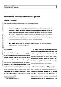
After all, it is reasonable that histories with K far from its typical value are characterized by different magnetizations. In other words, the ground state is highly nontrivial, as opposed to the high-temperature phase. In order to further illustrate our point, we have plotted s 7→ mK (s, β = 1.4) in Fig. (2). There it can be seen that mK (s, β) jumps from a nonzero value at s > 0 to zero at s < 0. On the one hand, at s > 0 one is probing the regime in which K/t is typically smaller than its average value hr(M)i, which we expect to be more frozen than typical configurations, that is, more ordered: this accounts for mK (s, β) growing with s. On the other hand, at s < 0, one is selecting histories that have a typical K/t larger than average, so that the corresponding states should be less ordered. There is in fact a dynamical first order phase transition as s varies from 0+ to 0− , where mK (β, s) jumps from a nonzero value to 0, which corresponds to a paramagnetic state. The jump discontinuity of mK (β, s) yields a discontinuity in the deriva-
mK (s, β)
s Figure 2: Plot of the rotation parameter mK (s, β) as a function of s at β = 1.4. The jump discontinuity at s = 0, in finite size N, is smoothened into a continuous but steep drop centered around a critical value sc = O(N −1 ) < 0. tive of ψK (which itself, being convex, must be continuous) as shown in Fig. (3),
33
which reads � � � � q d ψK (s) ψK (s) d (0) 2 lim lim − = 1 − m K + − ds N →∞ N ds N →∞ N 0 0 (0)
(0)
(120)
(0)
where mK = mK (β, 0)qis the solution to mK = tanh βmK . For finite N, both
derivatives are equal to
(0) 2
1 − mK . 1 ψ (z) N K 0.05
0.9
0.95
1.05
1.1
1.15
1.2
z
-0.05
-0.1
-0.15
-0.2
Figure 3: Plot of z 7→ limN →∞ ψK (z)/N at β = 1.4, with z = e−s . The first derivative is discontinuous at z = 1. Returning now to the topological pressure, we parallel the reasoning carried out previously for K in terms of Q+ : we write the corresponding operator W+ and perform a rotation of the magnetization operators M α (the angle θ involved is such that sin θ = m+ (β, s)) in order that it can be expressed in terms of free bosons, and we find that below the critical temperature ψ+ (s) = Nψ (N ) (s) + ψ (0) (s)
(121)
where the order N 1 and order N 0 coefficients are given by q (N ) (122) ψ+ (s) = p2−s q s − 2 s � �2s � �s � −(1+s) q q (0) s 2 ∆1 + ∆2 ψ+ (s) = q (1 − s) 1 − p β p − ∆0 + p p (123) 34
where we used the notation q p = 1 − m2+
(124)
q = 2 cosh βm+ − m+ sinh βm+
�
�
q = 2 sinh βm+ − m+ cosh βm+ � �2 ∆0 = − βm+ cosh βm+ + (1 − β) sinh βm+ � � ∆1 = −pβ (2 − β) cosh βm+ + m+ β sinh βm+ � 2 4s � ∆2 = 2 − 1 + 2 2 21 m+ qq − p2 (1 − p2 β)2 p pq
(125) (126) (127) (128) (129)
and the rotation parameter m+ (s, β) is the solution of � � � � p1+s βm+ cosh βm+ + (1 − β) sinh βm+ = q s−1 m+ q + sq(1 − p2 β) (130) such that ψ+ (s) is the largest. Again the quantity m+ (s, β) has the meaning of an average magnetization biased, for s 6= 0, over histories that are more (resp. less) random than the typical history for s > 0 (resp. s < 0). For that reason we expect m+ (s, β) to be a decreasing function of s, as is confirmed by plotting m+ (s, β) obtained from (130) as a function of s for β > 1, see Fig. (4). Trajectories split into two classes, ordered and disordered ones. This splitting is not present in the unbroken phase (β < 1), for which m+ (β < 1, s) = 0 ∀s.
6.3 Kolmogorov Sinai entropy and chaoticity Here we focus on the KS entropy related to the process M(t) – and defined as before from the QM observable –, which is luckily extensive. In the stationary � � state, hKS (in magnetization space) depends on β through c = cosh β m(β) where m(β) is the solution of the mean field equation ln 2 if β < 1 1 lim (131) hKS = 1 N →∞ N ln 2 if β > 1 c
To follow how hKS depends on β in the high temperature phase (β < 1) one has to expand up to order 0. We find hKS − N ln 2 = −
1 + (ln 2 − 1)β(2 − β) 2(1 − β) 35
(132)
m+(s, β)
s Figure 4: Plot of s 7→ m+ (s, β) at β = 1.4 in the limit of large systems.
hKS − N log 2 0 -1 -2 -3 -4
1 N hKS
0.8
0.6
disordered phase
0
0.2 0.4 0.6 0.8 β
0.4
0.2
ordered phase
0.5
1
1.5
2
2.5
3
β
Figure 5: Kolmogorov-Sinai entropy hKS in the stationary state, as a function of β. In the ordered phase (β > 1), the variations of hKS are of order N, while in the disordered phase, they are of order 1 (inset).
36
Results are shown in Fig. (5). In a state P of average magnetization m, hKS [P ] only depends, to leading order in N, on m. � � � � 1 1 + m −2β m 1 − m 2β m −βm 1 + m βm 1 − m +e hKS [P ] = e ln 1 + e ln 1 + e N 2 1−m 2 1+m (133) In a similar way � � � � 1 R 1 − m 2β m 1 + m −2β m −βm 1 + m βm 1 − m +e h [P ] = e ln 1 + e ln 1 + e N KS 2 1+m 2 1−m (134) 1 N hKS
0.8
hKS and chaoticity are decreasing
0.6
hKS and chaoticity are increasing
equilibrium magnetization
0.4
0.2
0.2
0.4
0.6
0.8
1
m
meq
Figure 6: Kolmogorov-Sinai entropy hKS [P ] in a state P of mean magnetization m at fixed β = 1.2.
6.4 On the extensivity of the KS entropy Though the hKS associated with the observable QM and calculated in the previous section was luckily extensive, in general the hKS defined by (20) is not extensive ′ in the number of degrees of freedom. Indeed, the dominant order for hKS = ψ+ (0) obtained from (105) reads hKS ∼ N ln N. By contrast, in a dynamical system, the Lyapunov spectrum, and the KS entropy, are extensive in the number of degrees of freedom. The nonextensivity of the hKS calculated in this paper was already briefly commented upon in Sec. 4.3. As this was pointed out in Sec. 5.1.2, it is not specific to continuous time. Still, we wish here to suggest some possible cures. In 37
1 N hKS 1 R N hKS
1 0.8 0.6 0.4 0.2
-1
-0.5
0.5
1
m
Figure 7: Direct and time-reversed Kolmogorov-Sinai entropies in a state of mean magnetization m, in the disordered phase (β = 0.8). Notice that, as expected, hKS ≤ hR KS . These two dynamical entropies are equal only at equilibrium magnetization meq = 0.
1 h N KS 1 R h N KS
1 0.8 0.6 0.4 0.2
-1
-0.5
0.5
1
m
Figure 8: Direct and time-reversed Kolmogorov-Sinai entropies in a state of mean magnetization m, in the disordered phase (β = 2). Notice that, as expected, hKS ≤ hR KS . These two dynamical entropies are equal only at equilibrium magnetization meq ≃ ±0.956 or at m = 0, which is unstable.
38
order to obtain an extensive topological pressure, we may scale the probability of a step from C → C ′ with the number of available degrees of freedom. In the case of our Ising system, we introduce the observable H=
K−1 X n=0
ln
NW (Cn → Cn+1 ) r(Cn )
(135)
Note that the associated large deviation function ψH (s) = limt→∞ 1t lnhe−sH i, in spite of remaining convex, will a priori no longer be a monotonously increasing function of s, which is a defining property of a Rényi entropy. Skipping technical details, we have found that in the high temperature phase ψH (s) = 1 − β(1 − s) −
p √ β=1 (1 − s)(1 − β)2 + s, ψH (s) = s − s
(136)
which has a trivial thermodynamic limit ψH /N → 0 as N → ∞. On the other hand, for β > 1, we obtain √ ψH (s) = (r(Nm)/N) − p(r(Nm)/N)s , p = 1 − m2 N
(137)
and with m solution to m(r(Nm)/N)s − mpβ cosh βm − p(1 − β) sinh βm = 0
(138)
Combining these results into a single plot, Fig. (9), shows that some features present in ψ+ (such as ψ+ (s > 0) = 0) are unaffected in ψH (s): both are monotonous (only to leading order in N for ψH (s)), and non-analytic in s = 0. We do not have further argument in favor of using ψH /N as a bona fide topological pressure but that it is simple and that it seems to be sharing similar properties as ′ the original ψ+ , at least for the model at hand (yet it can be shown that ψH (0) ≤ 0, i.e. opposite sign to hKS ).
6.5 One dimensional Ising model We consider an Ising chain of N spins in contact with a thermal bath at inverse temperature β. The energy writes X H=− σi σi+1 (139) i
39
1 ψ (s) N H
s Figure 9: Plot of s 7→ limN →∞ ψH (s)/N at β = 1.4. We endow the system with periodic boundary conditions and Glauber dynamics with spin flip rate Wi (σ) = 1 −
1 γ σi (σi−1 + σi+1 ) 2
where
The Kolmogorov-Sinai entropy is + * X Wi (σ) hKS = Wi (σ) ln r(σ) i
γ = tanh 2β
(140)
(141)
In the limit N → ∞ � � N ln N +N 2βγ tanh2 β −(1+γ 2 ) ln cosh 2β +2 sinh2 β +O(ln N/N) cosh 2β (142) r which is computed using that the correlations read hσi σi+r i = tanh β. It is, as expected, an increasing function of temperature.
hKS =
40
7 Physical example 4: Contact Process 7.1 Motivations We now turn our attention to the infinite-range contact process: each vertex i of a fully connected graph of N vertices is either empty (ni = 0) or occupied by a particle (ni = 1). The system is endowed with a Markov dynamics with rates ( � W ni = 1 → ni = 0 = 1 � (143) W ni = 0 → ni = 1 = λn/N P where n = i ni is the total number of occupied sites. This model has recently resurfaced in the literature: Dickman and Vidigal [46] studied in detail one of its defining properties, namely that it exhibits a nonequilibrium phase transition from an active to an absorbing state as the branching rate λ is decreased below a critical value λc = 1, with, in finite size, a single stable state, the absorbing one. Therefore, the stationary state distribution in the active state is only quasistationary. The lifetime of the active state, in finite size, was studied by Deroulers and Monasson [47], who also designed a systematic way to implement finite connectivity effects. Broadly speaking, the contact process phase transition belongs to the directed percolation universality class, and as such, is the paradigmatic model of nonequilibrium phase transitions. Our motivation for looking at the contact process with our own tools is precisely the existence of a phase transition, unlike any equilibrium one, that is encountered in many guises in the literature (see Hinrichsen for a review [48]). Interestingly, absorbing state transitions are now invoked within the framework of the glass transition [49, 50, 51]. At the moment we do not wish to address refined critical properties, and we shall be content with a mean-field version that will enable us to get the global picture of how phase space trajectories are affected by the presence, in the stationary state phase diagram, of an absorbing state transition. Much like the global magnetization in the infinite-range Ising model, the total P number of particles n(t) = i ni = 0, . . . , N is also a Markov process, with the following rates ( W (n → n − 1) = n (144) W (n → n + 1) = (N − n)λn/N As a reminder, we first sketch the main properties of the stationary state. For finite N, there is a single stationary state: this is the absorbing state where all sites are 41
empty. The time evolution of the mean number of particles reads � � dhni λn = (N − n) −n dt N
(145)
Given the infinite range of the interactions, the mean field hypothesis will be valid in the thermodynamic limit (n and N going to infinity, n/N → ρ). In the stationary state (145) simplifies into � � ρ λ(1 − ρ) − 1 = 0 (146)
We conclude that there exist two regimes according to the value of λ. For λ ≤ 1, the stationary state is the absorbing state, with all sites devoid of particles, and when λ > 1, the system reaches almost certainly a quasi-stationary state with mean density 1 ρ=1− , (147) λ else it is trapped in the empty state. From here on, we shall assume λ > 1 and use ρ as the only control parameter of the model. In order to circumvent the absorbing state in finite size, it is convenient to add to the original model an additional local injection process with rate h, ( � W ni = 1 → ni = 0 = 1 � (148) W ni = 0 → ni = 1 = h + λn/N or
(
W (n → n − 1) = n W (n → n + 1) = (N − n) [h + λn/N]
(149)
The stationary state becomes unique for N → ∞, and the steady-state density ρ is given by λρ + h = ρ/(1 − ρ) (150) For h > 0, explicit results will be expressed in terms of ρ and λ. We now want to determine the large deviation functions of K(t), the number of configuration changes that have occurred over a time interval [0, t], and of Q+ (t), which gives access to the topological pressure.
42
7.2 Special point λ =
2ρ−1 (1−ρ)2
Our first paragraph deals with a special point in parameter space that, to the best of our knowledge, has never been commented upon in the existing literature, but whose mathematical structure is extremely simple. We decompose the total number of particles into an average and a fluctuating part, √ (151) n = Nρ + ξ N and we express the fluctuating rate of escape from a configuration with n particles, in the stationary state. In the absence of particle injection (h = 0), and replacing λ by its expression (147) in terms of the stationary state density ρ, we arrive at r(n) = 2ρN + ξ
1 2 − 3ρ √ N − ξ2 1−ρ 1−ρ
(152)
hence the special point ρ = 2/3 (or equivalently λ = 3) at which this escape rate has relative fluctuations of order O(N −1 ) that are much weaker than the generically expected O(N −1/2 ). A similar phenomenon occurs for h > 0, using (150), √ r(n) = 2ρN + ξ(1 − ρ)(λ − Λ) N − λξ 2 (153) where Λ=
2ρ − 1 (1 − ρ)2
(154)
There the special point with low fluctuations is at λ = Λ. Under this constraint λ = Λ, the interval covered by the stationary state density when the value of h is varied is 12 < ρ < 32 . The λ = Λ behavior of r(n) bears much resemblance with that already noted for the high-temperature phase of Ising model in (109), with the formal correspondence β < 1 ↔ λ = Λ and β > 1 ↔ λ 6= Λ. As will now be seen, huge calculational simplifications occur at λ = Λ. The generating function for the cumulants of K(t), the number of configuration changes that have occurred over a time interval [0, t] is the largest eigenvalue of the following operator � � � � � � λˆ n 1 λˆ n x y x y WK (z) = −ˆ n+(N−ˆ n) + h + z (M + iM ) + h + (M − iM ) N 2 N (155) 43
where n ˆ = (N + M z )/2 is the particle number operator and z = e−s . Given that the detailed properties are being studied for the first time here, we shall provide the reader with a few more technical details than in the previous section on the Ising model. The spectrum of WK can be found perturbatively in N using the HolsteinPrimakoff representation of the magnetization operators M α . In general this consists in rewriting the M α ’s as a carefully chosen rotation of another set Lα of spin N operators for which we will use the following exact representation in terms of creation and annihilation operators Lx = N − 2a† a
(156)
�1 �1 iLy = a† N − a† a 2 − N − a† a 2 a �1 �1 Lz = a† N − a† a 2 + N − a† a 2 a
(157) (158)
The aforementioned rotation has to be chosen such that in the ground state, a† a remains small, so that an expansion can be performed. In the present case (λ = Λ), we shall assume that it is already the case without any rotation, and we shall use directly M α = Lα . We expand WK in powers of N anticipating that in the ground state a† a will remain of O(1) as N → ∞. And because, up to a constant contribution, WK is quadratic in terms of a and a† (with N-independent coefficients), this is indeed the case and we find that the largest eigenvalue ψK (s) of WK has the following expression Root of a third degree polynomial if z < zc 1/2 p ψK (z) = 2ρ (z − 1) N − z + z ρ(1 − 2ρ) + z(1 − 3ρ(1 − ρ)) if z > zc 1−ρ (159) 2ρ−1 provided the parameters verify λ = (1−ρ)2 . Note that for h = 0, that is at λ = 3, p zc = 1 and ψK (z ≤ 1) = 0, while ψK (z) = 43 (z − 1)N − z + z(3z − 2) if z > 1. Interestingly, to leading order in N, the distribution of K is a Poissonian, as was precisely the case for the Ising model in the high-temperature phase (111). For h 6= 0, we find that for z → 0 (that is for s → ∞) ψK (z) = ρ
2 − 3ρ 2 − 3ρ + z2 + O(z 4 ) 2 (1 − ρ) 2(1 − 2ρ)
(160)
which describes reduced-activity histories with values of K much smaller than 44
hKi. P In much a similar way, restricting our analysis to the Markov process n(t) = i ni (t), the topological pressure ψ+ (s) is the largest eigenvalue of the following operator −W+ (s) =ˆ n + (N − n ˆ)
λˆ n N
�1−s � �s � 1 λˆ n λˆ n x y − (M + iM ) h + n ˆ+h+ 2 N N �s � 1 λˆ n − (M x − iM y ) n ˆ+h+ 2 N
(161)
And again expanding the M α ’s in powers of N keeping a and a† of order 1, leads to W+ being quadratic in a and a† , with N-independent coefficients. Using the Bogoliubov-like transformation described in Appendix A, it is thus a simple matter to find the largest eigenvalue of W+ , which reads 2ρ (2s − 1)N + 2s (1 − s) s � � 1 − 3ρ(1 − ρ) ρ(1 − 2ρ) s ψ+ (s) = − 4s − s + 2 + O(1/N) if s ≥ sc (1 − ρ)2 (1 − ρ)2 − hN + O(1/N) if s ≤ sc (162) is given by where h = (2−3ρ)ρ . The critical value s that emerges in (162) c (1−ρ)2 � p λρ 1 1 � −2 + log2 λρ + λρ − log2 λρ + O(1/N 2 ) + 2 N 2ρ ln 2 (163) √ When s > 0, the expansion of the W+ is valid only when s ≪ N. When N is (large and) fixed, the asymptotics of ψ+ (s) is � �s √ hN 2 + 2λρN − λ as s → ∞ (164) ψ+ (s) ∼ hN N sc = log2
In Fig. (10) we have plotted ψ+ (s) as a function of s. The most remarkable feature is the presence of dynamical transition at the critical parameter s = sc . The nontrivial convex branch ceases to correspond to the largest eigenvalue of W+ at s < sc , and it is simply replaced by a plateau. This picture, which is customary 45
1 ψ (s) N +
1
0.5
-5
-4
-3
-1
-2
1
s
-0.5
-1
Figure 10: Topological pressure limN →∞ N1 ψ+ (s) on the special line (at ρ = 0.57). The dashed line is the continuation of the strictly convex branch for s < sc . in equilibrium phase transitions, reflects the existence of an underlying first order transition. As s is decreased from s = 0 (corresponding to typical histories) one is selecting histories with less and less dynamical disorder. This indicates a phaseseparation like mechanism occurring in the space of histories. We now attack the generic case for which the values of h and λ are unrestricted.
7.3 Generating function of the number of events for any λ The task remains that of finding the largest eigenvalue ψK (s) of WK as given in (155). When directly expanded in N, the choice M α = Lα leads to the following expression for the evolution operator WK �√ � √ (1) ˆ (0) + O( N ) N +H (165) − WK (z) = H (2) N + Ha(1) a + Ha† a† (1)
(1)
ˆ (0) is quadratic in a and a† . While where H (2) , Ha , Ha† are c-numbers and H (1) this seems a perfectly legitimate large N expansion, the presence of nonzero Ha (1) or Ha† terms in (165) signals that the ground state of −WK does not correspond to the zero boson state, but rather to an O(N) boson state (on the special parameter subspace Λ = λ these coefficients of the linear terms in a and a† somehow
46
miraculously vanish). Indeed, in order to compute that spectrum we need√ to trans2 late the creation and annihilation operators by a constant of magnitude N, but this mixes the whole expansion (165) of WK (z) in powers of N. In particular, (1) (1) unless Ha = Ha† = 0, the truncated expansion (165) is not sufficient to find the eigenvalues of WK (z), even to lowest order in N. Given that we wish to describe −WK ’s low lying excitations, with a† a ∼ O(1), we must now find a way to expand around the ground-state. By contrast to Ruijgrok and Tjon [45], we must now perform two successive rotations parametrized by α and m (around the y and the z axes) of the initial Holstein-Primakoff representation (156-158). The evolution operator WK (z) then reads � � λˆ n 1 n x y λˆ −1 x y − WK (z) = n ˆ + (N − n ˆ) − z α (M + iM ) + α (M − iM ) N 2 N (166) y y with M = L , ( � � x� � x� � √ −1 ≤ m ≤ 1 p −m L M , p = 1 − m2 and = z z L m p M α≥0 (167) (1) The parameters of the two rotations, α and m, will now be chosen so that Ha = (1) Ha† = 0 in the truncated expansion (165) of (166). When these equations in α and m have more than one solution, we have to choose the solution which gives the highest value of ψK .qExpanding WK (z) in powers of N and imposing (1)
(1)
1−ρ and yields an expression of the form (165) Ha = Ha† implies that α = 2 1+m with � q � 1 (2) 1 4pz 2 (1 + m)(1 − ρ) − (3 − 2ρ − m)(1 + m) H = (168) 4(1 − ρ) � � q 1 (1) (1) 1 Ha = Ha† = z(3m − 1) 2 (1 + m)(1 − ρ) + p(1 − ρ − m) 2(1 − ρ) (169) (1)
(1)
From (169) we see that solving Ha = Ha† = 0 in m leads to either m = −1 or m is one of the roots of third degree polynomial. If m = −1 is not the correct ˆ (0) to solution, this root must be inserted back into the expressions of H (2) and H get ψK (s). With a view to avoiding further technicalities, it is more convenient to 2
for instance, through similarity transformations such as eCa a† e−Ca = a† + C.
47
use algebraic elimination methods so as to find an equation on H (2) itself, and on ˆ (0) . Skipping details, one finds that when m 6= −1, H (2) is the coefficients of H one of the roots of the following polynomial P (X) = c3 X 3 + c2 X 2 + c1 X + c0 c3 = 16(1 − ρ)2
(170)
c2 = −27 z 4 (−1 + ρ)3 + 12 z 2 (−1 + ρ)2 (−4 + 3 ρ) − 8 −6 + 12 ρ − 7 ρ2 + ρ3 � c1 = −12 z 4 (−1 + ρ)2 (−4 + 3 ρ) − z 2 96 − 228 ρ + 184 ρ2 − 53 ρ3 + ρ4 � + (−2 + ρ)2 12 − 12 ρ + ρ2 � �2 c0 = (1 − z 2 ) 4z 2 (1 − ρ) − (2 − ρ)2
We first consider the case s ≥ 0. In that range of s, we see that by definition (1) (1) we must have ψK (s) ≤ 0. However, the solution m = −1 of Ha = Ha† = 0 yields ψK (s) = 0, which is the highest possible value of ψK (s). We thus have ψK (s) = 0 in the whole s ≥ 0 range. We now assume s < 0. And again by definition we must have ψK (s) ≥ 0. The solution m = −1 still yields ψK (s) = 0. We thus have to check whether P (X) has any negative solution. The discriminant of P (X) has the simple form ∆=−
228
�2 1 z 2 2 + z 2 (−1 + ρ) − ρ 5 (1 − ρ) n � o3 �2 3 24z 2 (1 − ρ) + ρ2 + 12ρ − 12 + (6 − ρ)3 (−2 + 3 ρ)
33
(171)
As ∆ < 0 in the range s < 0, P (X) has three real valued roots. Moreover, from the coefficients of (170) it is easy to see that the roots of P (X) have a positive sum and a negative product, which shows that P (X) has only one negative root, namely, H (2) . From Cardano’s formula, setting q = (9c1 c2 c3 − 27c0 c23 − 2c32 )/(54c33 ) we find3 that in the range s < 0 (2)
ψK (s) = −
� � � 13 � 13 √ √ c2 + e2iπ/3 q + i −∆ + e−2iπ/3 q − i −∆ 3 c3
(172)
As a remark, we notice that the two rotations of parameters α and m could also be understood as the result of suitable similarity transformations of the kind 3
The expression of ψK takes real values but can’t be written with algebraic operations involving only real quantities: this is the casus irreductibilis of Cardano’s formula.
48
�
z
z
eθM (. . .)e−θM performed on WK (z) before expanding in N. In other words, finding the roots of (170) enabled us to perform an appropriate resummation of (165) to all orders in order to obtain a series whose truncation to lowest order has well defined spectrum, which makes the large N expansion consistent. In order to be more explicit, we now provide the limiting behavior of ψK (s) = (2) (0) NψK (s) + ψK (s) + O(N −1 ) in two limits of interest, namely for s → 0− , h 2 s3 (−4 + ρ (4 + ρ)) (2) −s 2 s ψK (s) = 2ρ(e − 1) + (2ρ − 3) − ρ ρ3 s4 (432 + ρ (−1248 + ρ (1188 + ρ (−444 + 79 ρ)))) i + O(s5 ) 12 ρ5 and for s → −∞,
(2)
lim es ψK (s) = 1
s→−∞
The remaining O(1) piece in ψK is given by (0)
ψK (s) = C +
√
D
(173)
(174)
where C is a root from the polynomial P = z 2 (−2 + ρ)2 + 4 z 4 (−1 + ρ) − 2 X 3 (−1 + ρ)2
� − X z 2 (−1 + ρ) ρ + 4 X 2 (−1 + ρ) 3 z 2 (−1 + ρ) + 2 ρ
(175)
and D is a root from the polynomial
� P = 256 X 3 (−1 + ρ)5 + 16 X 2 (−1 + ρ)3 −27 z 4 (−1 + ρ)2 + 24 z 2 (−1 + ρ) ρ − 4 ρ2 � � − z 2 (−2 + ρ)2 + 4 z 2 (−1 + ρ) 108 z 4 (−1 + ρ)2 + 8 ρ3 − 9 z 2 (−1 + ρ) (−12 + ρ (12 + ρ)) + � 8 X z 2 (−1 + ρ)2 −108 z 4 (−1 + ρ)2 − 8 ρ3 + 9 z 2 (−1 + ρ) (−12 + ρ (12 + ρ)) (176) It is now time to summarize our findings, which we do in the following two plots Figs. (11) and (12), showing respectively the full plot of ψK (s) as a function of s and that of the density ρ(s) = (1 + m(s))/2 corresponding to the rotation parameter m(s) as a function of s. On Fig. (11) we notice that ψK (s) is not analytic at some critical point sc which corresponds to the phase-separation like mechanism depicted by the topological pressure ψ+ (s) (see Fig. 10), but now at the level of the number of events 49
1 ψ (s) N K
0.2
-0.6
-0.4
-0.2
0.2
0.4
0.6
s
-0.2 -0.4 -0.6 -0.8 -1
Figure 11: Plot of limN →∞ ψK (s) as a function of s at λ = 2 and h = 0.3. Note the presence of a jump in the first derivative at s = sc ≃ 0.16.
ρ(s) 0.6
0.5
0.4
0.3
0.2
0.1
-0.6
-0.4
-0.2
0.2
0.4
0.6
s
Figure 12: Plot of ρ(s) = 1+m(s) in the N → ∞ limit as a function of s at λ = 2 2 and h = 0.3. Note the presence of a jump at s = sc ≃ 0.16.
50
K. This result illustrates that this simple quantity – at least for infinite-range systems – already contains much of the information given by Q+ on the complexity of histories. This is fully confirmed by Fig. (12). In analogy to the Ising case (119), ρ(s) = 1+m(s) represents the mean density in the biased state P˜K (n, s): 2 ρ(s) =
1 X ˜ nPK (n, s) N n
(177)
As usual, at s = 0 we recover the density in the steady state. At s < 0 we probe the regime in which the mean “activity” K/t of histories is typically larger than in the steady state. They correspond to explored configurations where the density is larger than the steady state density ρ. On the other hand, at s > 0 histories with smaller K/t are favored. Increasing s leads to a sudden jump in the typical density, which corresponds to a dramatic change in the kind of configurations explored by histories with reduced activity K/t.
7.4 Topological pressure: h = 0 We begin by attacking the h = 0 case for which the phase diagram possesses two stationary states, the active and the absorbing one. The topological pressure ψ+ (s) is the largest eigenvalue of the operator W+ (s) written out in (161). By techniques similar to those mentioned above, we arrive at (N )
(0)
ψ+ (s) = Nψ+ (s) + ψ+ (s)
(178) s
!
2q s r (179) + 1−ρ (1 + m)(1 − ρ) s 1 + m 2q s (1 + m) (0) ψ+ (s) = (1 − s) (180) 4p 1−ρ v s u u � 2q s (1 + m) q s 1 + m p ∆0 + s∆1 + s2 ∆2 (181) + − t− 4(1 − ρ) 1−ρ 4 1−ρ (N )
ψ+ (s) =
1+m 4
−
51
where we used the notations √ p = 1 − m2 r = 3 − m − 2ρ r2 q= 2(1 − m)(1 − ρ) 3 1 ∆0 = + 2 1−m � 2s ∆1 = 2 p2 − 2r(1 + m − ρ) r (1 + m)(1 + m − 2ρ)2 ∆2 = − 2(1 − m)r 2
(182) (183) (184) (185) (186) (187)
The rotation parameter m is the solution of p 2pr(1 − m − ρ) = 2(1 − ρ)(1 + m)q s (s(1 + m)(1 + m − 2ρ) + (1 − 3m)r) (188) such that ψ (N ) (s) has the largest value. The first cumulants can be determined without toil, � � 1 ρ 1 1−ρ hQ+ i = 2ρ ln 2 − −8 ln 2 + O(1/N 2 ) (189) Nt 4N 1 − ρ ρ 1 (2 − 3ρ)2 hQ2+ ic = ρ(ln 2)2 + (ln 2)2 + O(1/N) (190) Nt ρ (191) Fig. (13) shows the topological pressure ψ(s) and the corresponding density ρ(s) is represented on Fig. (14).
7.5 Topological pressure (ii): h > 0 Finally we turn to h > 0 for which the explicit formulas read ψ(s) = Nψ (N ) (s) + ψ (0) (s) √ � 1 −r + 2p r q s ψ (N ) (s) = 4 r q � (1 − s)u qs (0) ψ (s) = − q s ∆0 + s∆1 + s2 ∆2 2p r 52
(192) (193) (194)
1 N ψ+ (s)
1 0.8 0.6 0.4 0.2
-0.2
0.2
0.4
0.6
s
Figure 13: Plot of the topological pressure limN →∞ N1 ψ+ (s) as a function of s at λ = 5 and h = 0. Note the presence of a jump in the first derivative at sc = 0.
ρ(s) 0.8
0.6
0.4
0.2
-0.2
0.2
0.4
0.6
s
as a function of s at λ = 5 and h = 0 in the large Figure 14: Plot of ρ(s) = 1+m(s) 2 system limit N → ∞. Note the presence of a jump at sc = 0.
53
where we used the notations √ p = 1 − m2 � r = 2 2h + λ(1 + m) r = 12 (1 − m)r + 2(1 + m) r q= 2 rp
(195) (196) (197) (198)
u = 4h + λ(1 + m)2 ∆0 =
(199)
h λ p2 + m λ 2 p2 + 2+ 4r p 2 1−m
(200)
� � ∆1 = 4 h (1 + m)2 λ −4 + (1 − m)2 λ + 4 h2 −8 + (1 − m)2 (1 + m) λ (201) 3 2 2� + (1 + m) λ −4 − 2 (1 + m) λ + (1 − m) λ (202) �2 2 r − 4(1 + m) u ∆2 = − (203) 4rp2 r2 and m is the solution of � � √ pr(h + λm − 1) r = su r − 4(1 + m) + r 4hm − λ(1 + m)(1 − 3m) (204) such that ψ (N ) (s) has the highest value. The values of the first two cumulants read " # 1 1 1 8λρ(1 − ρ)2 2 λ− hQ+ i = 2ρ ln 2 + − �2 ln 2 + O(1/N ) Nt 4N 1−ρ 1 − λ(1 − ρ) (205) � � 2 1 − 2ρ + λ(1 − ρ)2 1 hQ2+ ic = ρ(ln 2)2 + ρ (ln 2)2 + O(1/N) (206) Nt 1 − λ(1 − ρ)2 (207) The contact process also raises interest [47] in related computationally motivated problems where similar absorbing-state phase transitions have been identified. We believe that not only the KS entropy, but also the pieces of information contained in P˜+ or P˜K , could shed a new light, with quantitative tools, on dynamical complexity issues. 54
8 Outlook Before concluding, we would like to discuss [52] on a simple example, namely Brownian motion, the difference between the Markov approach we were dealing with in this paper, and another possible approach which also generated a lot of literature in the field of dynamical and chaotic properties of systems. Let us first adopt the Lorentz gas picture [19] in which a particle is scattered by randomly placed obstacles. Over large distances, the particle is seen to perform a diffusive motion. Furthermore, two infinitesimally close-by particles will quickly follow exponentially diverging routes. This is a chaotic system. A Lorentz gas is well approximated by a Markov process. The possibility of choosing a variety of infinitesimally close initial conditions, leading to very different trajectories, is replaced with the drawing of random numbers whose net effect is to account for the chaotic nature of the Lorentz gas. Within this approach, such local characterization of chaos like individual Lyapunov exponents cannot be accessed. An opposite approach to Brownian motion is the modeling in terms of a Langevin equation, say for the particle velocity, which evolves under the effect of an external position independent – yet random – force. Within this picture [53, 54, 55], the random force is viewed as an external field. Two close-by initial conditions will be subjected to the same realization of the random force. Within this picture, a simple Brownian motion is not a chaotic system. What can possibly make it chaotic lies in space-dependent forces due to interactions or to an external field. The difference in the two pictures lies in the observation scale compared with the intrinsic correlation length of the surrounding medium. In the first approach, the noise source is very short range correlated in space, but with long range time correlations. In the second approach, this is the exact opposite situation. When computing a Lyapunov exponent, before deciding which picture applies, one must compare the typical physical scales of the medium giving birth to a chaotic behavior. For times short with respect to the correlation time scale and distances large with respect to the correlation length, the first approach – the Markov one – applies. If this is the case, we have shown that the thermodynamic formalism can successfully be applied to Markov dynamics with continuous time, provided that the proper interpretation is used for the definition of the dynamical partition function. In particular, a finite KS-entropy can be defined. This opens the door to explicit expressions for realistic systems. Besides, we have embedded this formalism into a more general picture. Indeed, the dynamical partition function can be expressed as the generating func55
tion of an observable. By noticing that other observables could be used as well, we are able to relate the quantities used in the thermodynamic formalism with those involved in the much studied Lebowitz-Spohn [8] fluctuation theorem. We also show on specific examples that the simplest observable one could think of, namely the number K of transitions occurring in a given time, is not as trivial as one could think and contains already some relevant information on the system. For example, for the infinite range Ising model, the cumulant generating function of K already indicates that a dynamical phase transition occurs in the low temperature phase. This is confirmed by the calculation of the more sophisticated topological pressure. We found also that one can gain some insight into these dynamical phase transitions by looking at a new object: the aforementioned cumulant generating function was obtained as the largest eigenvalue of a certain operator. If one also computes the associated eigenvector, one can build a quantity that weights the trajectories depending on the value the observable takes along them. In the example of the infinite range Ising model, this allows to show that the dynamical phase transition which occurs below the critical temperature gives rise to a splitting of the trajectories into two families, respectively typical of a disordered and of an ordered phase. The general unifying picture behind all this is that of a Gibbs ensemble construction carried out over the space of dynamical trajectories, rather than over microscopic states. We have illustrated our approach on several physical examples (an interacting lattice gas, a system exhibiting an equilibrium second order phase transition and one with a nonequilibrium phase transition). Our setup has allowed us to provide an intrinsically dynamical picture to phenomena that are always interpreted in static terms. This constitutes a powerful tool that longs to be applied to systems for which no static phenomena has ever been identified, like those possessing glassy dynamics. It is tempting to speculate that ageing and other dynamical features of glasses will be identified with a sharp signature on some appropriately chosen dynamical potentials like those considered throughout this work. Some of these ideas can already be found in [56, 57]. But before addressing these challenging issues, many questions remain to be answered for more conventional systems. As far as lattice gases are concerned, the general dependence of the KS entropy on the diffusion constant and the compressibility is one such question. Driving a lattice gas into a nonequilibrium steady-state (with a bulk or boundary field) leads to distinct dynamical features. How do these reflect on the dynamical partition 56
function? In the vicinity of a second-order transition, the dynamics possesses universal features, so that the dynamical potentials ψA (s) introduced in this paper will obey universal scaling laws. Which are these? May be some universal scaling functions as the one found in [12] could emerge. The influence of quenched disorder, generically known to slow the dynamics down is one more open research route. Acknowledgments: The authors wish to thank T. Delattre for his participation in the early stage of this work, along with J. Tailleur, J. Kurchan and H. van Beijeren for their many helpful critical comments.
A Non-hermitian quadratic operators and Bogoliubovlike transformation Holstein-Primakoff expansions of our evolution operators WA for infinite-range ˆ that is quadratic in creation and annihimodels often lead to a “Hamiltonian” H † lation operators a and a ˆ = Xa2 + 2Za† a + Y (a† )2 H
(208)
ˆ In order that the latter exists we We are interested in the lowest energy level of H. shall have to assume that ∆2 = Z 2 − XY > 0 and Y ≤ 0. Performing the similarity transformation P1−1 (. . .)P1 with P1 = e
Z−∆ 2 a 2Y
(209)
does not alter a while it shifts a† according to P1−1 a† P1 = a† −
Z −∆ a Y
(210)
ˆ Its purpose is to remove the a2 term in H: ˆ 1 = P −1 HP ˆ 1 = Y (a† )2 + 2∆a† a + ∆ − Z H 1
(211)
We now introduce the operator Y
† )2
P2 = e− 4∆ (a 57
(212)
It commutes with a† and shifts a according to P2−1 aP2 = a −
Y † a 2∆
(213)
ˆ 1 , it yields Acting on H ˆ 2 = P −1 HP ˆ 2 = 2∆a† a + ∆ − Z H 2
(214)
As the similarity transformations (210) and (213) do not modify the spectrum ˆ ˆ of H(s), we see that the lowest energy level of H(s) is ∆ − Z. When H is Hermitian (X = Y ), the Bogoliubov transformation leads to exactly the same result. However, when H is not Hermitian, the Bogoliubov transformation cannot be implemented: contrary to (210) and (213), it does not transform a and a† independently, which was required here to obtain (214).
58
References [1] D. Ruelle, Thermodynamic Formalism, 1978, Addison-Wesley, Reading (Mass.). [2] Ya. G. Sinai, Russian Mathematical Surveys 27, 21 (1972), Gibbs measures in ergodic theory; D. Ruelle, Am. J. Math. 98, 619 (1976), A measure associated with axiom-A attractors; R. Bowen and D. Ruelle, Inventiones Mathematicae 29, 181 (1975), The ergodic theory of axiom-A flows. [3] G. Gallavotti and E.G.D. Cohen, Phys. Rev. Lett. 74, 2694 (1995) [chao-dyn/9410007], Dynamical ensembles in nonequilibrium statistical mechanics. [4] D. J. Evans and D. J. Searles, Phys. Rev. E 50, 1645 (1994), Equilibrium microstates which generate second law violating steady states. [5] C. Jarzynski, Phys. Rev. Lett. 78, 2690 (1997) [cond-mat/9610209], Nonequilibrium equality for free energy differences. [6] C. Bustamante, J. Liphardt and F. Ritort, Physics Today 58, 43 (2005), The non-equilibrium thermodynamics of small systems; F. Ritort, in Poincaré Seminar 2, 195-229 (Birkhäuser Verlag, Basel, 2003) [cond-mat/0401311], Work fluctuations, transient violations of the second law and free-energy recovery methods: Perspectives in Theory and Experiments; G. M. Wang, E. M. Sevick, E. Mittag, D. J. Searles, and D. J. Evans, Phys. Rev. Lett. 89, 050601 (2002), Experimental Demonstration of Violations of the Second Law of Thermodynamics for Small Systems and Short Time Scales; G. M. Wang, J. C. Reid, D. M. Carberry, D. R. M. Williams, E. M. Sevick, and D. J. Evans, Phys. Rev. E 71, 046142 (2005), Experimental study of the fluctuation theorem in a nonequilibrium steady state; G. M. Wang, D. M. Carberry, J. C. Reid, E. M. Sevick and D. J. Evans, J. Phys. Condens. Matter 17, S3239 (2005), Demonstration of the steady-state fluctuation theorem from a single trajectory; K. Feitosa and N. Menon, Phys. Rev. Lett. 92, 164301 (2004), Fluidized Granular Medium as an Instance of the Fluctuation Theorem; S. Ciliberto, N. Garnier, J. F. Pinton and R. Ruiz-Chavarria, Physica A 340, 240 (2004), Experimental test of the Gallavotti-Cohen fluctuation theorem in turbulent flows; S. Ciliberto and C. Laroche, J. Physique IV 8 , Pr6-215 (1998), An experimental test of the Gallavotti-Cohen fluctuation theorem; N. Garnier and 59
S. Ciliberto, Phys. Rev. E 71, 060101 (2005), Nonequilibrium fluctuations in a resistor. [7] J. Kurchan, J. Phys. A 31, 3719 (1998) [cond-mat/9709304], Fluctuation theorem for stochastic dynamics. [8] J.L. Lebowitz and H. Spohn, J. Stat. Phys. 95, 333 (1999) [cond-mat/9811220], A Gallavotti-Cohen Type Symmetry in the Large Deviation Functional for Stochastic Dynamics. [9] G. E. Crooks, J. Stat. Phys. 90, 1481 (1998), Nonequilibrium Measurements of Free Energy Differences for Microscopically Reversible Markovian Systems; Phys. Rev. E 60, 2721 (1999) [cond-mat/9901352], Entropy production fluctuation theorem and the nonequilibrium work relation for free energy differences. [10] C. Giardinà, J. Kurchan and L. Peliti, Phys. Rev. Lett. 96, 120603 (2006), Direct evaluation of large-deviation functions. [11] B. Derrida and J. L. Lebowitz, Phys. Rev. Lett. 80, 209 (1998) [cond-mat/9809044], Exact large deviation function in the asymmetric exclusion process. [12] B. Derrida and C. Appert, J. Stat. Phys., 94, 1-30 (1999) Universal large deviation function of the Kardar-Parisi-Zhang equation in one dimension. [13] T. Bodineau and B. Derrida, Phys. Rev. Lett., 92, 180601 (2004) [cond-mat/0402305], Current fluctuations in nonequilibrium diffusive systems: an additivity principle. [14] V. Lecomte, Z. Rácz and F. van Wijland, J. Stat. Mech., P02008 (2005) [cond-mat/0412547], Energy flux distribution in a two-temperature Ising model. [15] J. Farago, J. Stat. Phys. 107, 781 (2002) [cond-mat/0106191], Injected Power Fluctuations in Langevin Equation. [16] F. van Wijland and Z. Rácz, J. Stat. Phys. 118, 27 (2005) [cond-mat/0404358], Large deviations in weakly interacting driven lattice gases.
60
[17] V. Lecomte, C. Appert-Rolland and F. van Wijland, Phys. Rev. Lett. 95, 010601 (2005) [cond-mat/0505483], Chaotic properties of systems with Markov dynamics. [18] P. Gaspard, Chaos, scattering and statistical mechanics, Cambridge Nonlinear Science Series vol. 9 (Cambridge UP, 1998). [19] J.R. Dorfman, An introduction to chaos in nonequilibrium statistical mechanics, Cambridge University Press, Cambridge, 1999. [20] J.R. Dorfman, M.H. Ernst and D. Jacobs, J. Stat. Phys. 81, 497 (1995), Dynamical chaos in the Lorentz lattice gas. [21] C. Appert, H. van Beijeren, M.H. Ernst and J.R. Dorfman, Phys. Rev. E 54, R1013 (1996) [chao-dyn/9607019], Thermodynamic formalism in the thermodynamic limit: Diffusive systems with static disorder; C. Appert, H. van Beijeren, M.H. Ernst and J.R. Dorfman, J. Stat. Phys. 87, 1253 (1997) Thermodynamic formalism and localization in Lorentz gases and hopping models [22] P. Gaspard, J. Stat. Phys. 117, 599, (2004), Time-Reversed Dynamical Entropy and Irreversibility in Markovian Random Processes. [23] C. Beck and F. Schlögl, Thermodynamics of Chaotic Systems: An Introduction, Cambridge Nonlinear Science Series vol. 4 (Cambridge UP, 1993). [24] N. van Kampen, Stochastic processes in physics and chemistry (NorthHolland, 1992). [25] H. van Beijeren and J. R. Dorfman, Phys. Rev. Lett. 74, 4412 (1995), Lyapunov Exponents and Kolmogorov-Sinai Entropy for the Lorentz Gas at Low Densities. [26] H. van Beijeren, J. R. Dorfman, H. A. Posch and Ch. Dellago, Phys. Rev. E 5 6, 5272 (1997) [chao-dyn/9706019], Kolmogorov-Sinai entropy for dilute gases in equilibrium. [27] M. Dzugutov, E. Aurell, and A. Vulpiani, Phys. Rev. Lett. 81, 1762 (1998), Universal Relation between the Kolmogorov-Sinai Entropy and the Thermodynamical Entropy in Simple Liquids; E. G. D. Cohen L. Rondoni , Phys. Rev. Lett. 84, 394 (2000), Comment on Universal Relation between the 61
Kolmogorov-Sinai Entropy and the Thermodynamical Entropy in Simple Liquids; A. Samanta, Sk. M. Ali and S. K. Ghosh, Phys. Rev. Lett. 92, 145901 (2004), New Universal Scaling Laws of Diffusion and Kolmogorov-Sinai Entropy in Simple Liquids; D. Ihm, Y.-H Shin, J.-W. Lee and E.K. Lee , Phys. Rev. E 67, 027205 (2003), Correlation between Kolmogorov-Sinai entropy and self-diffusion coefficient in simple fluids. [28] Z. Rácz, SPIE Proceedings 5112, 248 (2003) [cond-mat/0307490], Scaling functions for nonequilibrium fluctuations: A picture gallery. [29] B. Derrida, B, Douçot and P.-E. Roche, J. Stat. Phys. 115, 713 (2004), [cond-mat/0310453], Current fluctuations in the one dimensional symmetric exclusion process with open boundaries. [30] H. van Beijeren and J. R. Dorfman, J. Stat. Phys. 108, 767 (2002), [nlin.CD/0112031], A note on the Ruelle pressure for a dilute disordered Sinai billiard. [31] P. Gaspard and X.-J. Wang, Phys. Rep. 235, 291, (1993), Noise, chaos, and (ǫ, τ )-entropy per unit time. [32] P. Gaspard, J. Stat. Phys. 88, 1215, (1997) Entropy production in open volume-preserving systems. [33] A. Latz, H. van Beijeren and J. R. Dorfman, Phys. Rev. Lett. 78, 207 (1997), Lyapunov spectrum and the conjugate pairing rule for a thermostatted random Lorentz gas: kinetic theory. [34] P. Grassberger, private discussion. [35] D. J. Evans, E. G. D. Cohen, and G. P. Morriss, Phys. Rev. Lett. 71, 2401 (1993), Probability of second law violations in shearing steady states. [36] D.J. Evans and D.J. Searles, Adv. Phys. 51, 1529 (2002), The Fluctuation Theorem. [37] C. Maes, J. Stat. Phys. 95, 367 (1999) [math-ph/9812015], The fluctuation theorem as a Gibbs property. [38] L. Bertini, A. De Sole, D. Gabrielli, G. Jona-Lasinio and C. Landim, [cond-mat/0407161], Macroscopic current fluctuations in stochastic lattice gases. 62
[39] L. Bertini, A. De Sole, D. Gabrielli, G. Jona-Lasinio and C. Landim, [cond-mat/0506664], Non equilibrium current fluctuations in stochastic lattice gases. [40] L. Bertini, A. De Sole, D. Gabrielli, G. Jona-Lasinio and C. Landim, [math.PR/0512394], Large deviations of the empirical current in interacting particle systems. [41] M.H. Ernst and J.R. Dorfman, Chaos in Lorentz Lattice Gases, in 25 Years of Non-Equilibrium Statistical Mechanics, p. 199-210, J.J. Brey, J. Marro, J. M. Rubi and M. San Miguel Eds., (Springer Verlag, Berlin, 1995). [42] P. Gaspard and G. Nicolis, Phys. Rev. Lett. 65, 1693 (1990), Transport properties, Lyapunov exponents, and entropy per unit time. [43] B. Derrida, Phys. Rep. 301, 65 (1998), An exactly soluble non-equilibrium system: the asymmetric simple exclusion process. [44] D. Kim, Phys. Rev. E 52, 3512 (1995) Bethe ansatz solution for crossover scaling functions of the asymmetric XXZ chain and the Kardar-Parisi-Zhangtype growth model. [45] Th.W. Ruijgrok and J.A. Tjon, Physica 65, 539 (1973), Critical slowing down and nonlinear response in an exactly solvable stochastic model. [46] R. Dickman and R. Vidigal, J. Phys. A 35, 1147 (2002), Quasi-stationary distributions for stochastic processes with an absorbing state. [47] C. Deroulers and R. Monasson, Phys. Rev. E 69, 016126 (2004) [cond-mat/0309637], Field theoretic approach to metastability in the contact process. [48] H. Hinrichsen, Adv. Phys. 49, 815 (2000) [cond-mat/0001070], Nonequilibrium Critical Phenomena and Phase Transitions into Absorbing States. [49] R.H. Schonmann, J. Stat. Phys. 58, 1239 (1990), Critical points of twodimensional bootstrap percolation-like cellular automata. [50] J. Reiter, F. Mauch and J. Jäckle, Physica A 184, 493 (1992), Blocking transitions in lattice spin models with directed kinetic constraints. 63
[51] C. Toninelli, G. Biroli and D.S. Fisher, Phys. Rev. Lett. 96, 035702 (2006) [cond-mat/0509661], Jamming Percolation and Glass Transitions in Lattice Models. [52] Julien Tailleur, private discussion. [53] R. Graham, Europhys. Lett. 5, 101 (1988), Lyapunov exponents and supersymmetry of stochastic dynamical systems. [54] E. Gozzi and M. Reuter, Chaos, Solitons & Fractals 4, 1117 (1994), Lyapunov exponents, path-integrals and forms. [55] S. T˘anase-Nicola and J. Kurchan, J. Phys. A 36, 10299-10324 (2003) [cond-mat/0210380], Statistical-mechanical formulation of Lyapunov exponents. [56] M. Merolle, J.P. Garrahan and D. Chandler, Proc. Nat. Acad. Sc. 102, 10837 (2005), Space-time thermodynampics of the glass transition. [57] R.L. Jack, J.P. Garrahan and D. Chandler, [cond-mat/0604068], Spacetime thermodynamics and subsystem observables in a kinetically constrained model of glassy systems.
64
1 N hKS
0.8
0.6
0.4
0.2
-1
-0.5
0.5
1
m