procedures for the collection of data on salience, to propose a tool ââthe fenceâ â for estimating the effects of changes in salience on voting shares and finally to ...
Early Draft, All Comments Welcome
Thinking About Salience Macartan Humphreys and John Garry March 2000 ABSTRACT Political scientists agree that salience matters. What they don’t agree about is what exactly salience is, how it relates to preferences, and how to measure it. Nor do they have analytic tools for understanding how system-wide changes in salience affect social choice. In this paper we begin by discussing three rival concepts of relative salience. We note that for all three interpretations preferences are a function of salience. But note that these three –often confused– interpretations have different implications for data collection. We then turn to questions of social choice. We develop a set of propositions that identify the conditions under which rankings over pairs or triples of alternatives will be invariant to changes in salience and when rankings depend uniquely on salience parameters. We examine the types of changes in salience that are required to reverse an individual’s or a group’s ranking. Finally we consider voting. For situations where social choices are not invariant to relative salience we demonstrate how we can map from changes in salience to changes in vote shares for any two policy options. It turns out that even for two alternatives in only two dimensions such mappings are not monotonic. To help demonstrate the relevance of the results we consider the election of John Major to the head of the British conservative party in the early 1990s and formally examine the role that salience played in that election. The paper aims to shed light on a foggy debate, to urge for more theoretically informed procedures for the collection of data on salience, to propose a tool –“the fence” – for estimating the effects of changes in salience on voting shares and finally to provide some theoretical foundations for Riker’s notion of heresthetics. 1 2
Introduction .................................................................................................................. 2 Ideas of Salience ........................................................................................................... 3 2.1 The Classical Interpretation: Separability of Salience and Ideals............................. 3 2.2 The Valence Interpretation: Identity of Salience and Ideals .................................... 7 2.3 The Price Interpretation: Ideals as a Component of Salience................................. 11 2.4 When Interpretations Meet Data .......................................................................... 15 3 Theoretical Issues: When and How Salience Matters for Social Choice and Voting ...... 21 3.1 Invariance to Changes in Salience........................................................................ 21 3.2 Salience Cycles ................................................................................................... 26 3.3 Introducing the Fence and its Rotations................................................................ 35 3.4 Non-Linear Fences .............................................................................................. 39 4 Applications ............................................................................................................... 42 4.1 Application to the 2-dimensional Case ................................................................. 42 4.2 Examples with Simulated Data ............................................................................ 43 4.3 Empirical Application: Choosing a Leader for the British Conservative Party....... 47 5 Conclusion.................................................................................................................. 52
1
1
Introduction “Would you tell me please which way I ought to go from here?” “That depends a good deal on where you want to get to,” said the Cat. “I don’t much care where ” said Alice. “Then it doesn’t matter which way you go,” said the Cat. “ so long as I get somewhere, ” added Alice as an explanation.
Salience – the relative importance of different policy areas – is one of the primitives of political modeling. Any study that aims to understand the wheeling and dealing that takes place within and between political coalitions in any institutional environment has to take account not just of what people think about different issue areas but how much they care about them. Any study that tries to understand how political actors get their way in elections or in committees has to take account of where those actors stand. But they also have to take account of what issues have been made into important issues, and what issues have been marginalized or avoided outright. The importance of salience has been recognized by political scientists in some form or another for a long time. Theories that try to model “political manipulation” or “heresthetics,” for example, claim that politicians may do well by attempting to change the relative salience of different issues.1 From a theoretical point of view, however, the study of salience has been all but ignored. Two research agendas need to be addressed by political scientists. The first agenda should set about understanding when and how salience and changes in salience matter for political action. The second should endogenize changes in salience, it should examine the ability of political actors to change the relative importance of different issue areas2. This paper falls within the remit of the first agenda. In this study we aim to examine from a formal theoretical point of view when and how changes in salience really make a difference to policy choice and when politicians may have an incentive to try to overplay or underplay the relative salience of different issue areas. In the first part of this paper we consider three related interpretations of salience. The first, which we call the “classical interpretation”, derives from early work in spatial modeling. It is a concept of salience that is independent of players’ ideal policies and the location of the status quo. The second notion, which we call the William Riker (1986), The Art of Political Manipulation, New Haven: New Haven University Press. Understanding why different issues are on or off the political agenda has indeed been central to many positive studies of politics without being couched in the language of salience or spatial modeling. An important focus of Horowitz’s work on ethnicity, for example, is his study of the institutions that make intra-ethnic issues more salient relative to inter-ethnic issues: Donald Horowitz, (1985), Ethnic Groups in Conflict, London: University of California Press. Understanding the sources of relative salience is also of considerable normative importance, see for example Drèze and Sen’s frustration at the failure of famines to be high on the political agenda: Jean Drèze and Amartya Sen (1989) Hunger and Public Action, Oxford: Clarendon Press, Chapter 13.7.
1
2
2
“valence interpretation,” formalizes the notion that for some issues salience is position. More precisely, we show that for some types of issues over which there is general consensus regarding ideals, the salience of issues in an unconstrained game uniquely determines the policy position in a constrained game. The third interpretation, which we call the “price” interpretation, lies somewhere between the first two. It formalizes the notion that salience refers to an agent’s willingness to trade off policy across a number of dimensions. Under this interpretation salience can not be considered independently of ideal points, but salience and ideals are not identical either. We end this section by considering how these rival interpretations affect data collection and interpretation. We criticize methods that have been used to collect data on salience and the ways that such data has been related to theory. We link different procedures to collect salience data with interpretations of salience and suggest ways to collect salience data. The rest of the paper concentrates on concepts developed during our discussion of the first interpretation. It considers the effects of changes in salience. We will see that focusing on changes allows us to produce results that are consistent with both the classical and price interpretations of salience. Since in the classical conception salience is not globally separable from preferences, we begin by inquiring into the conditions under which knowledge of relative salience is required in order to determine an individual’s ranking of policy alternatives. We then turn to examine the types of changes in salience that are required to reverse an individual’s ranking. Next we examine majority rule, and under very general conditions we determine the conditions under which knowledge of salience is necessary to rank social alternatives. For situations where social choices are not invariant to relative salience we demonstrate how we can map from changes in salience to changes in vote shares for any two-policy options. Interestingly, it turns out that such mappings may not be monotonic. In other words, as a policy dimension increases in salience a policy or candidate may initially benefit in terms of increased support but as salience continues to increase, support may then start to decrease. In the final section we try to bring some of the results to life. We give a mathematically simpler analogue of the general results for the two dimensional case. We then provide some examples of the propositions in action, two with simulated data and one with data from the British Conservative Party. The paper aims to shed light on a foggy debate, to urge for more theoretically informed procedures for the collection of data on salience, to propose a tool –“the fence” – for estimating the effects of changes in salience on voting shares and finally to provide some theoretical foundations for Riker’s notion of heresthetics.
2 2.1
Ideas of Salience The Classical Interpretation: Separability of Salience and Ideals
In spatial models of policy choice we typically assume players think of some set of policies as being ideal. We will treat this set of policies as a point, p, in n-dimensional policy space. For economists, p is a point of global satiation. A player’s feelings regarding any existing or proposed policy vector, say x, are given in a general manner by the distance between p and x. The measure of distance, however, may depend on how
3
the player weights different dimensions or upon the way her preferences on one dimension depend on the location of policy on another dimension. Davis et al3 propose a general utility function of the form ui = vi((x-p)TA(x-p)), where vi(.) is any player-specific function, that is monotonically decreasing in (x-p)TA(x-p). The function reports only ordinal utility information. A is a symmetric n×n positive definite matrix with typical element aij, and with aii ≥ 0, it carries information regarding the weights that players attach to different dimensions. It will be useful for what follows to define a symmetric matrix Σ = [σ σij] such that ΣΣ = A. We shall refer to utility functions of this form as “classical” (spatial) utility functions. It is common in spatial modeling to treat indifference curves as Euclidean, that is, to use Euclidean distance as the relevant metric. This assumption means that a player’s feeling about a policy is a function of ((x-p).(x-p)).5. In terms of the general functional form, Euclidean indifference curves correspond to the special case where A = In×n, the n×n identity matrix. Hence we may write ui(x) = vi((x-p).(x-p)) = vi([x1- p 1]2 + [x2- p 2]2 +… + [xn- p n]2) Equation 1
It is easy to see that since vi(.) is strictly monotonic, the set of points given by vi(.) = k will be a set of points, {x}, such that r = (x1 – p1)2 + (x2 – p2)2 +…++ (xn – p n)2 Equation 2
where r = vi-1(k). This we recognise to be the equation for a circle (or sphere, hypersphere). Hence “Euclidean preferences” implies circular indifference curves. Note now that if we apply a nominal stretch of policy space by premultipling all points by Σ-1, then (x-pi)'A(x- pi) = (x- pi)'ΣΣ (x- pi) becomes (Σ-1x-Σ-1 pi)'ΣΣ (Σ-1x-Σ-1 pi) = (Σ-1(x- pi))'ΣΣΣ-1 (x- pi) = (x- pi)'Σ-1ΣΣΣ-1 (x- pi) = (x- pi)'In×n(x- pi). That is, we can induce Euclidean preferences for any given player by an appropriately chosen stretch of policy space. This holds whether or not preferences are separable across dimensions4. The stretch may of course have less elegant effects on the indifference curves of other players! Now, if we only impose the restriction that aij = 0 ∀ i≠j then A will be a diagonal n×n matrix. As long as all dimensions matter, A will be non-singular. In this case Equation 1 will read: ui(x) = vi(a11[x1-p1]2 + a22[x2-p2]2 +… + ann[xn-pn]2) = vi([σ11(x1-p1)]2 + [σ22(x2-p2)]2 +… + [σnn(xn-pn)]2) Equation 3
The analogue of Equation 2 will read: 3 Otto Davis, Melvin Hinich and Peter Ordeshook (1970), “An expository development of a mathematical model of the electoral process”, American Political Science Review, 64, pp. 426 - 449. 4 Note that to derive this we only required the symmetry and invertibility of Σ.
4
k = a11[x1-p1]2 + a22[x2-p2]2 + … + ann[xn-pn]2 Equation 4
which we recognize to be the equation for an ellipse (ellipsoid). Furthermore, in this case, the aii or σii have a natural interpretation. In particular, as is evident from the second equality in Equation 3, σii gives a weighting for the distance between x and p along dimension i. This is the classical spatial interpretation of salience, the statement “dimension i increased in salience by a factor ε” means precisely σii increased by factor ε, ceteris paribus. Note especially that this concept is independent of the player’s ideal point and of the status quo. It is probably this policy-independent notion of salience that Dahl had in mind as the basis of his theory of polyarchy5. A player will prefer one option y, to another, x, if: a11[y1-p1]2 + … + ann[yn-pn]2 < a11[x1-p1]2 + … + ann[xn-pn]2 Equation 5
If for convenience we normalize p at the origin, this condition, in matrix notation, is: a.[y2 -x2] < 0 Equation 6
where x2 and y2 are vectors with typical elements xi2 and yi2 and a is a vector containing the diagonal elements of A, with a > 0. The condition can be interpreted either as reading that y will be preferred to x only if [y2-x2] lies below a hyperplane through the origin with directional vector a, or as reading that y will be preferred to x only if a > 0 lies below a hyperplane through the origin with directional vector [y2 -x2]. The latter interpretation will be useful in Section 2.4 for calculating values for a.6 z
z
y x
z
y p
x
y p
World I
Dimension I
x
p
World II
Dimension I
World III
Dimension I
Figure 1
It should be clear that under this interpretation of salience, changes in salience effect a change in preferences. That is, even though salience is logically distinct from ideal points, it is not logically distinct from preferences more generally understood. Indeed an Robert A. Dahl (1956), A Preface to Democratic Theory, Chicago: University of Chicago Press. It is worth noting the relationship the left hand side of Equation 6 and econometric formulations of binary choice problems. The left hand side of the equation is an index function with the constraint that the elements of a are positive. 5
6
5
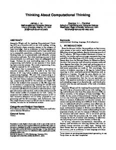
individual’s attitude towards a policy is, as we have seen, a function of both salience and her ideal point. The following graphical example should make this clear. Consider the ranking of options x, y and z for player P in Figure 4 The positions of x, y and z are marked such that if P had Euclidean preferences, as in the diagram in the first panel, then she would prefer y to both x and z. And she would prefer x to z. This is captured by the circle centered on P’s ideal point, passing through y and the distances of x and z from it. All points inside the circle are preferred by P to y; all points outside of the circle, x and z in particular, are less preferred by P to y. If instead P felt that Dimension II was more important that Dimension I, then – were P to bargain between policy dimensions – we would, ceteris paribus, expect her to give up a relatively small amount of policy on Dimension II in exchange for a large policy shift on Dimension I. In terms of the diagram, we would now expect her indifference curve to be elliptical, stretched horizontally, relative to that in World I. We can now see, using the same logic as before, that A prefers option x to option y, and prefers option y to option z. If instead P valued Dimension II relatively more, she would have elliptical indifference curves stretched vertically, as in World III. In this case, we would see that P prefers z to y and y to x. Let us represent the preference rankings of P over the three options, x, y and z, explicitly. World I y x z
World II x y z
World III z y x Table 1
It is evident from Table 1 that given P’s ideal point, which of x, y and z is most preferred by P depends entirely on the relative salience of the two dimensions. If we do not have information regarding the salience, we would be unable to make determinate statements regarding the rankings of these alternatives. If we also allow for non-separable preferences we can easily generate majority rule cycles in just two dimensions, even when all three players have the same ideal point Hence differences in salience alone are enough to create indeterminacy in social rankings under majority rule. In section 3.2 we show how extreme this indeterminacy may be. We simply state here that in n dimensions with non-separable preferences, any n generally distributed points (not including the player’s ideal point) may be ranked in any order, depending on the salience weights! Hence preferences over a given set of options are not independent from the salience of the dimensions over which those options are defined. This point is simple but easily missed. In particular this means that if we believe that in their manifestos parties may reveal information about policy options on the table rather than their “ideals” we must accept that salience may affect a party’s position on an issue.7 It may for example be the case that parties take a stance on a series of options {x1, x2, …xj…xk} that constitute a strict subset of policy space. The subset may be the set of feasible policies, policies that happen already to be on the political agenda, or policies that are given by the strategies of their opponents. If the party’s own ideal point is not in the set {xj} we will need to provide an argument for why we believe that the party’s stated “substantive positions” are invariant to changes in salience.
7
6
Knowledge of salience, however, is not always necessary in order to know how a player ranks a set of alternatives. In Section 3.1 we describe the conditions under which such information is necessary.
2.2
The Valence Interpretation: Identity of Salience and Ideals
In Section 2.1 we interpreted a player’s ideal point as being a point of global satiation. The existence of such a point was simply assumed. Its existence is necessary to speak reasonably of a “policy position” in many contexts. In many political situations, however, it may seem unreasonable to simply assume that players have points of global satiation. If, for example, policy space were composed of allocations of resources to education, defense or the environment, would it not be more reasonable to assume that most players would really like to see as much expenditure on all areas as possible? Why vote for less when they can vote for more? Many distributive and expenditure games have this non-satiation aspect to them. However, these games are also characterized by constraints. All players may like to see enormous sums of money spent in every constituency and on every policy area, but they will eventually have to deal with budget constraints. How they choose to allocate resources in the presence of constraints will depend on how much they care about the different issues on the table – in other words, on the relative salience of the issues for the players. Hence salience in an unconstrained game may determine ideal points in a constrained game. We formalize these ideas next. We want to stress, however, that what follows relates to very particular types of political situations. As should be clear from the discussions of the preceding sections, we are not providing a general case to support the notion that salience and position are indistinguishable. What follows applies to situations a) in which there is little or no political disagreement about ideal outcomes but b) where policy space is constrained – that is, to situations in which policies in one dimension affect the feasibility (and not the desirability!) of policies in another.8,9 In these situations we argue that salience and policy position may be indistinguishable. However, even in these situations a more classical notion of salience may still be useful in meta-games – that is, in games with multiple sets of constrained spaces. In situations where there are n dimensions along which funds may be spent, the set of feasible expenditures will typically lie on an n-1 dimensional plane10. A player’s Note that in these games policies do not have a determinate “antithesis”. The opposite of spending the entire budget on Dimension A may be any point from the large set of points that allocates the budget among all other goods. The closest we can get to an antithesis is to work with the dimensions of the type “S”-“Not S”. 9 Although we focus on budgetary constraints there are other constraints that could work in a similar way. For example, policy makers may believe that there is a well-defined trade-off between inflation and unemployment. Hence although “ideally” they might like to see low unemployment and low inflation, they may believe that they are constrained to choose a point along this trade-off line. Their induced ideal point will then be some point along the trade-off determined by the relative weights they place on unemployment and inflation. More abstractly, policy-makers may feel that there is an inherent trade-off between law and order and freedom of expression. Hence, although they may ideally like to see both increased law and order and freedom of expression, politically they may function with an induced ideal point in what they believe to be the trade-off space. 10 Assuming availability of the good in question and linear pricing. 8
7
induced “ideal point” is then her favored allocation. This point corresponds to her Marshallian demands from consumer theory and lies on the budget plane. The player’s induced indifference curves are given by sets of points lying on the budget plane that produce equal utility. A player works out what her ideal point is by maximizing U(x1, x2….xn), subject to the constraint that c.x = B and xi ≥ 0 ∀i, where ci is the price of good i and B is the government budget. 11 We can simplify the arithmetic by assuming that quantity units are chosen such that ci = 1 for all i and by normalizing the budget to B = 1. We then think of this as a general divide-the-dollar game in which players care about all allocations. Their unconstrained problem is to maximize U(x1, x2….xn-1, 1- x1-x2…-xn-1). We denote the solution to this problem as p, the player’s (induced) ideal point. When we think of ideal points in this way, there are two important points to be emphasized. First, the constrained utility function will generally not be a special case of the “general” utility function for spatial games provided by Davis et al. We will see below that indifference curves may be very irregularly shaped, they will not be circular, elliptical or even homothetic. Second, measures of salience in the unconstrained utility function are likely to determine both salience and the location of ideal points in the unconstrained game. Indeed the two are likely to be inseparable, and so for these games it is true that “emphasis is direction”. We now provide an example to illustrate these points. We will look at the case where players have Cobb-Douglas utility functions over public expenditure. We will see that salience in the unconstrained game is position in the constrained game, and that player’s indifference curves are irregularly shaped. We demonstrate, however, that despite the seeming irregularities, preferences are well enough behaved to allow us to use some standard tools from spatial modeling in these situations. The fact that the situation described in this section is common for political decision making and is not particularly unusual from a modeling point of view makes it all the more important that we be aware of the inseparability of salience and position in this context. We begin by assuming that the utility of a player in the unconstrained game may be written: ui(x1,x2…xn) = α1ln(x1) + α2ln(x1) + α3ln(x3)… αnln(xn) Equation 7
Here the utility function is strictly increasing in all arguments over the whole range of x. Each dimension has an associated weight, αi. These weights represent the elasticity of utility of the voter with respect to expenditure in the different policy areas. We hold that in the unconstrained game these weights correspond to the relative salience of the different dimensions and we assume that they are strictly positive12. We also assume that expenditure in all areas is strictly positive (but may be arbitrarily low). The constrained utility function is given by
11 Note that for simplicity we assume here that budgets are given exogenously and that the government does not save or borrow. 12 A pure distributive game might have α = 0 for all i but one. i
8
ui (x1,x2…xn) = α1ln(x1) + α2ln(x1) + α3ln(x3)… αnln(1-x1 – x2…-xn-1) Equation 8
We can see that the constrained utility function is not monotonic in all arguments. The Marshallian demands take a simple form: with Cobb-Douglas utility a voter would like to see dimension i receiving share αi/Σjαj of the total budget. If we normalize Σjαj = 1 then pi = αi. Hence for this utility function the ideal points of the constrained game are given by what we would reasonably take to be salience measures in the unconstrained game. The player’s constrained utility function may then be written: ui = p1ln(x1) + p2ln(x1) + p3ln(x3)… pnln(xn). Equation 9
This function has no measure for salience independent of the ideal points and clearly cannot be arranged to correspond with the general functional form described by Davis et al and used in Section 2.1. We give a graphic illustration for voters deciding how a budget is to be allocated over three policy areas in Figure 2.
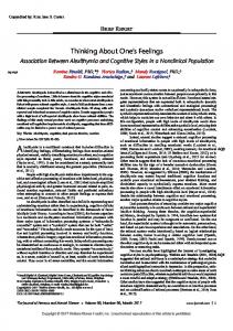
Four players and their indifference curves over expenditure in three policy areas with a fixed budget. Their salience weights are (.1, .4, .5), (.4, .4, .2), (.1, .1, .8), (.4, .1, .5), the first two weights correspond to the coordinates of the ideal point in the two dimensional space. A status quo position is marked with a dot.
9
Figure 2
For this figure, the budget constraints allow us to represent the game as a vote over expenditure in two policy dimensions, with the assumption that the residual is spent on the third. Alternatively, we may think of the vote as being the election of a minister of finance. A player’s ideal point, p, corresponds to a preferred share of revenues to be spent on dimension 1 and dimension 2 (with p1, p2 ∈ (0,1], and p1 + p2 < 1). The set of feasible policies then lie in a right-angled triangle, half a unit square. The figure shows indifference curves for four players with salience weights (.1, .4, .5), (.4, .4, .2), (.1, .1, .8), (.4, .1, .5). The ideal points of these four players form a square in two dimensions. We can see from the figures that for these players, the salience weights determine their ideal points, and also the shape of their indifference curves. It is impossible in this context to speak of a change in salience without either implying a change in the location of ideal points or disregarding the underlying functional form. Note that the classical interpretation of salience plays no role at all here. This draws attention to the dependence of the classical interpretation on a particular functional form, an important weakness of the interpretation. Lastly we remark that while the indifference curves in this setting are irregular, they do not make spatial modeling impossible. Indeed, it turns out that contract curves are still given by straight lines linking players’ ideal points. And the set of players that prefer a given policy y to some other policy x is still given by a hyperplane. Hence we can describe support bases for given policies in terms of half spaces, and even use the idea of a median hyperplane to develop general results. Essentially then, from a modeling point of view, we can use techniques developed in the Euclidean context very easily in this kind of game. Spend entire budget on policy Area 3
Spend entire budget on policy Area 1
Spend entire budget on policy Area 2
Four players vote over expenditure in three dimensions, each player has Cobb-Douglas utility with different weights on the three different dimensions. The figure shows induced ideal points on the budget plane and locates a point marked with a star that is unbeatable under majority rule. The point satisfies Plott’s conditions and is the only one in the policy space to do so.
Figure 3
We illustrate some of these points by reconsidering the four players from Figure 2. Since contract curves are still straight lines, and there are exactly four players, we can easily locate a stable “Plott” point: a point that is unbeatable under majority rule. This point is
10
illustrated in Figure 3. In this figure we superimpose the indifference curves we have already considered. We also rotate the space and re-stretch it for interpretative convenience. The re-stretchings results in a figure that treats the three dimensions symmetrically. It can be seen that for any pair of players, the set of tangencies of their indifference curves lie on a line through their ideal points. It follows from this and the fact that there are just four players, that there is a centrist point with an empty winset and hence a unique equilibrium. Clearly then in some situations it may well be the case that a reasonable interpretation of salience -how much a player cares about different areas of policy- is her ideal point. We have shown this starkly for expenditure situations, it could be true for other situations in which there are inherent trade-offs across policies. In our example a change in salience in an unconstrained game translated into a change in policy position in a constrained game. The classical concept is inapplicable in this situation. Finally, it should be noted that were this expenditure game only a sub-game of larger policy game the classical notion of salience could be reintroduced to describe different intensities of preference over expenditure and other policy areas.
2.3
The Price Interpretation: Ideals as a Component of Salience
In Section 2.1 we touched on the idea that salience captures the willingness of a player to trade off on one dimension in exchange for changes in policy in another. This idea was also in the background of our discussion in Section 2.2. Under both the classical and the valence interpretations, salience weighted gains in different dimensions differently. This implies that agents will trade off across different dimensions at different rates. In this section we focus more explicitly on trade-offs across dimensions. In doing do we develop and formalize a third rival notion of salience, the price interpretation. This notion is not separable from ideal points, but it is not equivalent to them either. It is more generally applicable than either the classical or valence interpretation, is politically more meaningful than the classical interpretation and, we believe, better describes the notion of salience that underpins the collection of much data on salience. To sharpen the distinction between a price interpretation and the classical and valence interpretations, we will consider a situation in which a set of players all have Euclidean preferences. Also for the sake of clarity we will assume that all players are equally dissatisfied with the status quo. We then ask: is it meaningful in this context to claim that different dimensions are more salient for different players? We have seen that under the classical interpretation it is not: each player finds each dimension equally salient. In particular, according to the classical interpretation, we cannot make statements of the form dimension j is more salient for B than it is for C. However, we argue that it may still be the case that a player “cares” more about one dimension relative to another in the sense that she will be willing to trade off more of one dimension in exchange for another than another player is. We argue that this provides the basis for a rival definition of salience, one that depends on information regarding ideal points. The rival notion of salience is nonetheless logically distinct from that of ideal points. To make this point more clearly we begin with an example in which three players, all equally dissatisfied with the status quo, all with Euclidean preferences, nonetheless weigh
11
different dimensions differently when contemplating a change in policy. We follow this up by formally identifying exactly what this concept of salience is. Consider Figure 4 below. In the first panel we locate a status quo and three players, P, B and C, each of whom is equally dissatisfied with the status quo. We then consider the following thought experiment: you want to move the status quo to the left by one unit, that is, you want the policy to lie somewhere on the line L. You want the support of one of the players P, B or C. None of the players would like to see the status quo moved to the left, so to gain their support you will you need to offer to shift the status quo south somewhat. You want to move the policy as little as possible to the south and so you decide to do some research. Your research consists in finding out which player will be the easiest to buy off. That is, you want to know for which player will you have to give away the least amount of the vertical dimension in exchange for a unit shift in the horizontal dimension. Ignorant of the classical definition of salience, and much to the consternation of spatial modelers, you conceive of your project as finding out for which player is the vertical dimension the most salient, and for whom is the horizontal dimension the least salient. L
SQ1
SQ1
C’s ideal
L
B’s ideal P
P’s ideal point
SQ2
SQ1
“Buying P”
SQ1
SQ1 C
L
L
B
“Buying B”
“Buying C” Figure 4
12
Your research produces the following. You find that P would happily give up a unit on the horizontal dimension in exchange for a one-unit shift on the vertical dimension. Indeed, she would accept as little as .27 units. The set of acceptable bargaining outcomes is given by the intersection of L and P’s preferred to set. It is not so easy to buy off player B however. B would have to be given a drop of exactly 1.73 units in the vertical dimension before she would find a one-unit shift to the left acceptable. Geometrically this is given by the tangency of L to B’s indifference curve. Player C is already unhappy with the status quo in terms of the horizontal dimension but very happy in terms of the vertical dimension. The final panel of Figure 4 shows that there is in fact no amount of change in the vertical dimension that would compensate her for a unit leftward shift. Geometrically this is given by the non-intersection of L and C’s indifference curve. As a result, you conclude that the horizontal dimension is least salient for player P and most salient for player C. Formally, the concept of salience described here is represented by the gradient of a player’s indifference curve at the status quo. To use an economist’s language we would say that the relative salience of a set of dimensions is given by the “marginal rate of substitution” between them. An indifference curve is simply a set of points, all of which give the same utility. More formally, for utility level k such a set of points is given by: ϑk = {x | u(x) = k}, where x is a vector in policy space. Totally differentiating u(x) = k gives an expression for the gradient of the indifference curve:
∂u ∂u ∂u dx1 + dx2 + ... + dxn = dk = 0 ∂x1 ∂x2 ∂xn Equation 10
In the 2 dimensional case the gradient can be written simply as:
dx 2 ∂u ∂u =− × dx1 ∂x1 ∂x 2
−1
Equation 11 To fix ideas, fix player P's ideal point at the origin, pi = 0 and let u(.) take the form discussed in section 2.1. Further assume that A is a diagonal matrix. Now the partial of ∂u ∂v u with respect to xi is given by = 2a ii x i . Hence Equation 11 becomes: ∂x i ∂x j ∂v dx 2 ∂v = 2a11 x1 2a11 x1 dx1 ∂x1 ∂x1
−1
=−
a11 x1 a 22 x 2 Equation 12
The slope is given by the slope of a circle, weighted by the relative “salience”. Evidently, the [x1/x2] term depends on the location of the status quo relative to the ideal point on a
13
dimension by dimension basis. Hence with (x1 – p1) = 0, the indifference curve is flat at x, with (x2 – p2) = 0 the curve is vertical. This provides one explanation for why extremists, players with ideal points very far away from the status quo on some dimension, may treat that dimension as being more salient13. We now highlight three properties of the price interpretation. First, the price interpretation is very generally applicable. It can be used in a much more general set of situations than the classical interpretation. Whereas we derived the classical interpretation by assuming a particular class of utility function, the price interpretation only requires that utility functions be differentiable at the status quo14. Hence for example, in Section 2.2 we saw that salience in the unconstrained game corresponds with ideals in the unconstrained game. We saw there that there was no way to make use of the classical conception of salience in the constrained game. We can, however, still make use of the price interpretation. For example, in the neighborhood of the status quo in Figure 2 (marked with a dot), the fourth player would hope for a reduction in expenditure on the vertical dimension. Indeed there is no feasible allocation of expenditure on the other two dimensions that would induce him to accept an increase in expenditure on the vertical dimension. What is more, he will accept an increase in expenditure on the third dimension only under the condition that it is financed by a cut in expenditure on the vertical dimension. Players two and three will trade off on the two dimensions approximately one for one in the vicinity of the status quo. But whereas player 3 will accept no cut in expenditure on dimension three, player 2 will accept no increased expenditure on that dimension. Second, the price interpretation has both ideals and the classical notion of salience as arguments. This fact provides the most important punchline for this section: to know to what extent a player will be willing to trade one dimension off against another we need to know not just the player’s relative weightings of different dimensions but also the relationship between the player’s ideal point and the status quo. Therefore under the price interpretation of salience, an individual-specific change in salience may be due either to a change in the location of the player’s ideal point or to a change in her A matrix. A more system-wide change in issue salience may be due to a correlated change in the A matrices across players, or more simply to a shift in the status quo. In the example given in Figure 4 above, an exogenous shift of the status quo to the south-east quadrant would reverse the saliences of the three players. Third, the price interpretation may be used to derive a ranking of dimensions. Agents may prioritize dimensions in order to decide where to concentrate their energies. That is, they may look to see where they get the greatest “bang for their buck”.15 Since the gain for a given change in policy in a given direction is given by the partial derivative of u with respect to that dimension, we can rank the salience of dimensions in the order of the magnitudes of their partial derivatives. Under this interpretation we say that Although see Section 3.4 for a more complete discussion of this point. The price interpretation for example could not be used in the case of lexicographic preferences. 15 Rabinowitz et al note that “any issue singled out as personally most important plays a substantially greater role for those who so view it than it does for others”. The finding, albeit rather trivial, points to the notion that agents may focus on a small number of dimensions where they believe the greatest gains in utility are to be had. George Rabinowitz et al (1982), “Salience as a Factor in the Impact of Issues on Candidate Evaluation”, The Journal of Politics, 44. 13
14
14
dimension i is more salient than dimension j if and only if ∂u ≥ ∂u , that is, if a unit ∂xi ∂x j change in dimension i, (from a given status quo, x) increases utility by more than a unit change in dimension j.16 Of course this ranking will not in general correspond to the ranking of the elements of the diagonal of the A matrix used for the classical interpretation.
2.4
When Interpretations Meet Data
We have considered three rival interpretations of salience. All three capture aspects of what we mean by “what issues people care about”, but in different ways. Rather than trying to decide which interpretation is the “true” meaning of salience we suggest simply that the concepts be consistently distinguished. In particular, it is very important that we be clear about which notion of salience corresponds to data that we collect on salience. We begin noting three problems that will affect data collection on salience no matter what interpretation is used. The first relates to the units that are used to measure dimensions. The second and third relate to the near ubiquitous conflation of salience data with information regarding other determinants of players’ behavior and with players’ uncertainty. We then turn to problems relating specifically to different methods of collecting salience data. First then, we should be aware of issues related to units. We said, for example, in our discussion of the price interpretation of salience that the order of magnitude of partial derivatives corresponded to salience rankings. The statement relied, somewhat naïvely on the notion of some natural scaling, where a unit of dimension 1 corresponded in some meaningful way to a unit of dimension 2. We cannot expect a natural scaling to exist and it would be unsatisfactory if salience rankings were reversed simply by choice of (in)appropriate units. Nonetheless, it should be noted that researchers have often assumed that if in their responses players assign the same score in some “importance” measure to two dimensions that their indifference curves over these two dimensions would be circular. To do this is to ignore the problem of units and to assume that there is some natural correspondence between endpoints on different dimensions. One way around the problem is to think of “more” or “less” salient as being valid conditional upon a given scaling. This solves the problem of the arbitrariness of units for any dimension but it does not help us with calculating relative salience. A better approach is to explicitly integrate scaling into salience questions. This is done in quite a subtle way in a technique used by Garry discussed and developed below. Finally, we can take heart in the fact that if our concerns are related to comparative statics, then percentage increases in relative salience will be unit independent. Next we consider the imputation of preferences from political behavior. In some cases data collection takes the form of examining the behavior of political actors — their voting behavior or their focus on different issues in writing or speech — to see into 16
We leave a discussion of what is meant by “a unit” to Section 2.4.
15
what dimensions they place their energies17. Before we map from behavior into preferences, however, we need to take account of the fact that an individual’s choice of dimensions to concentrate on is a choice. To understand an agent’s choice of concentration we need to consider not just the benefits deriving from a given change in policy but also the agent-specific costs of trying to influence policy in a given dimension. Some agents may be more capable of influencing policy in one dimension than in another. This will itself alter the extent to which they will lobby along that dimension. It should not be ignored, however, that if the data that is used to measure salience is based on political actors’ actions, such data is likely to conflate salience – under the price interpretation – with agent-specific costs. We should also be aware that data that derives from actions – revealed preferences – will include information not just regarding benefits and costs but also strategic considerations. It is possible for example that agents concentrate on particular dimensions in order to change the salience of those dimensions. It will be very clear from the results that follow that if political agents are able to alter salience, they will often have good cause to do so. It is also possible that actions are the outcome of a coordination game where some players concentrate on some dimensions while colleagues concentrate on other –-possibly more salient— dimensions. If at all possible it is important to distinguish empirically between emphasis deriving from strategy and emphasis deriving from salience.18 Lastly, we draw attention to the fact that data collected on salience may also conflate how much people care about an issue with how much they know about it. Indeed, at least locally, salience and certainty may be observational equivalents19. We propose a way of relating a person's certainty about what she likes in a given issue area with how much she cares about that issue area. We begin by reinterpreting the player’s "ideal point", p, as being the player's best guess, given the information she has, at what policy would suit her best. One way of thinking about this is that political actors may know what final outcomes they would like, but they are not sure what policies are the best ones to achieve those outcomes. Perhaps they want to alleviate poverty but do not know if this is done by raising the minimum wage or reducing it. We think of the player as playing a prior game in which she attempts to make a mapping from policies, x, to outcomes, y, based on a given history, öt. Her mapping may be more or less successful. Her own judgement regarding the For an early example of this see Douglas Rivers (1983), “Heterogeneity in Models of Electoral Choice”, Social Science Working Paper 505, Division of the Humanities and Social Sciences, California Institute of Technology. 18 Unless of course we can satisfy ourselves that an agent is constrained to treat the salience we infer from his actions as if it were his true salience. While such a move may be defensible in some contexts to ignore possible differences between a party’s stated and its “true” ideal points, the same case is difficult to make for salience. 19 This should make intuitive sense. Part of the oddness of Alice’s position in the opening quote is that she doesn’t have a preference over where she ends up, but still feels that where she ends up is an important issue. It does seem unusual to think of someone finding a given dimension extremely salient when that person doesn't know what policy she would like to see in place on that dimension. Why should a person care about a small change in policy from x1 to x1' when she isn't too sure whether she prefers x1 or x1'? 17
16
success of her mapping is captured by her estimates of her uncertainty surrounding her mapping. Once she has a mapping she estimate an ideal point and if she is smart she will incorporate her estimates of uncertainty regarding her mapping into her expectations of the payoffs from various policies. The agent will act then as if her ideal point has a multivariate distribution. The variance of the distribution will itself be a function of the size or length of öt and how good the player’s learning alogrithms are, that is, how sharp she is and how long she has been in the game. Let f(p|öt), describe the player’s estimated distribution of her estimated ideal point. A player weighing up different alternatives or contemplating trade-offs across dimensions will have to take account of this distribution. How she will do this will depend on their attitude towards risk20. For a general classical utility function, her expected utility will take the following form: Expected Utility =
∫ ...∫ ∫ pn
p2
p1
f ( p | ϕ t )v (( x − p)T A( x − p))dp1dp2 ....dpn
If the player is risk neutral (v''=0), the uncertainty may make no odds. If she is risk averse she will favor certain dimensions over uncertain dimensions ceteris paribus. In short, players will weight various dimensions or various combinations of dimensions differently. The result is that uncertainty may enter the expected utility function in a similar way to classical salience. If politicians get older and craftier of course, their observed salience should approach their "true" salience. -3
-3
0
0
-3
-3 -3
0
-3
-3
0
-3
A risk-averse player has a salience weighting of 8:1 in favor of the vertical dimension, but is uncertain over her preferred policy on it. Her ideal is distributed normal with µ =0 and σ2 =5.
A risk-averse player has “Euclidean preferences” but is uncertain over her ideal on one dimension. Her estimate of her ideal on the vertical dimension is distributed normal with µ =0 and σ2 =1.
Figure 5
In practice the interactions between uncertainty and salience are likely to be complex. To develop intuitions however Figure 5 provides two examples of indifference curves under uncertainty. For these cases we have assumed that the player is certain of Note that until now we have not had to make any assumptions regarding the shape of v(.). We no longer have this luxury, however, once we start taking uncertainty seriously. To do this, we assume utility functions are von-Neumann-Morgenstern. 20
17
her position on one dimension but uncertain on another. In particular we assume that her estimated ideal point is distributed normal. She is risk averse and has a classical spatial utility function. That is: Expected Utility =
∫
∞
−∞
f ( p2 | 0,σ 2 )v (a( x1 − p1 )2 + ( x2 − p2 )2 )dp2
The second panel in the figure illustrates the fact that for this specification the effects of uncertainty are dominant for policies close to the player’s (expected) ideal while salience dominates for options far from a player’s ideal. So much for general problems with salience data. We now turn to linking methods used for collecting data on salience with interpretations of salience. Data collected on salience oftentimes involves simply asking respondents questions of the form “which dimension is more important to you” or “how important to you is it that government continues or maintains its current policy”21. In these situations – assuming that responses are truthful – it is likely that we will be gathering information on the ordinal or sometimes cardinal ranking of dimensions, conditional on a given ideal point and status quo. Clearly, because of its dependence on ideal points and status quos, this method fails to provide direct information on salience interpreted classically, even though it is sometimes this interpretation that is supposed to provide the theoretical underpinning of the research22. Instead, these questions provide information on salience under the price interpretation. In the same way, subject to the caveats noted above, similar data deriving from a player’s actions are likely to capture salience as understood under the price interpretation. If such data is used for analysis it should be referred to hypotheses that derive from this notion of salience and not the classical notion. In particular, it should be noted that if responses to this type of policy change over time this does not mean that salience, understood classically, has changed. It may, however, be possible to use an expression such as Equation 12 to “back out” the classical notion of salience, the elements of the A matrix, from responses to questions of this form. We know of very few attempts to collect data that targets specifically the classical interpretation of salience. Econometric techniques to estimate classical salience weights for diagonal A matrices is discussed in Glasgow 199723. A related survey based method used by Garry (1995)24. In this work members of the British Conservative Party were asked to locate their ideal points and then asked to say how “close” they felt to different Such questions were used or example in the 1979 National Election Study Research and Development Survey discussed in Richard Niemi and Larry Bartels (1985), “New Measures of Issue Salience: An Evaluation,” The Journal of Politics, 47, pp. 1212-1220. 22 Richard Niemi and Larry Bartels, op cit., for example refer to the classical interpretation but use a methodology that is based on the price interpretation. 23 Garrett Glasgow, “Heterogeneity, Salience and Decision Rules for Candidate Preference.” Working mimeo. California institute of Technology. 24 John Garry (1995), “The British Conservative Party: Divisions Over European Policy”, West European Politics, 18: 4, pp. 170 – 189. 21
18
political leaders of the Conservative Party. As the ideal points of these leaders was also known, the approach gave information required to calculate a player’s metric. This approach has an affinity with early work in the study of neural networks to estimate a. We delay a presentation of this until after we introduce the notion of “the fence” in Section 3.3. For now we show how to use the approach for the case where a given player has a diagonal A matrix. The following presentation of the method is geometrical, and computationally easy. y2 y2-x2
y2-x2
y x2
x
H a
This figure represents a case where we have information regarding a player’s preferences over two points, x and y. x and y determine a line H = {z : z.(y2 -x2)=0}. If the player prefers y to x then we know that a lies on the unit circle somewhere below H. This area is marked bold in the third panel of the figure. Note that the area is well below the 45° line. This implies that the player cares considerably more about the horizontal direction (a1>a2) which is consistent with the fact that y is preferred to x.
Figure 6
Assume that we have data on a player’s ideal point and that her preference over some pair of alternatives, (x, y) is also known. We want to calculate the a vector in Equation 6, which we now think of as a point in the positive orthant of Rn. We can first of all normalize this vector so that it is of unit length, that is a.a = 1, geometrically this means that a lies on the unit sphere in the positive orthant. We can locate a hyperplane through the origin: H = {z : z.[y2 -x2] = 0}. If a player has classical separable preferences then from Equation 6 we know that if the player prefers y to x, then a lies on the unit sphere in the half space below H.25 If she preferred x to y then a would lie in the half space above H and so on. The more pairs over which we have preference information the more we can zoom in on the location of a. Furthermore different pairs zoom is on different areas of the unit sphere. The information from some pairs may repeat information from other pairs or it may complement it, depending on the location of the alternatives. In this way the geometry of the method can be used to guide the set of questions asked of respondents. In practice of course we may not have information regarding a player’s preferences over options in policy space and may want to use data
What if the hyperplane does not cut the positive orthant? This can happen in the case where the two dimensional vector (y2-x2) lies in the positive or negative orthants. In this case all values of a are consistent with one action and no values of a are consistent with another. Should a preference be voiced with which no value of a is compatible then our predictions based on spatial assumptions are incorrect. The failure may be passed off as noise, it may be an indication that the A matrix is not in fact diagonal or it may call for a fundamental questioning of the spatial assumption. See Proposition 1 below to see why a actions taken when H fails to cut the positive orthant may imply a violation of the diagonal A matrix assumption. 25
19
from past voting behavior. In this case we need to be aware of the various problems raised by revealed preferences discussed above. We provide an example of the technique just described in action for the case where we know an agent prefers y = (0,2) to x = (-1,1). This case is illustrated in Figure 6. Hence a relatively straight-forward method exists to collect data on salience that takes care of the unit problem and that may be used for either the price or classical interpretation. In short, we believe that extra care is needed in the production of salience measures, the interpretation of those measures and the linking of data so collected with theoretical work. The bad news is that most work done to date has failed to relate data collection exercises with clear conceptualizations of salience26 The good news from an analysis point of view, however, is the following: If we assume classical preferences, as is common in the spatial modeling literature, then both the classical and the price interpretations of salience use information from the A matrix in a similar manner. As a result comparative statics exercises that involve a change in salience while ideal points and status quo policy remain unchanged should lead to the same kind of results no matter which interpretation is adopted. For this reason we concentrate on the changes in the A matrix in the sections that follow.
This could be a major reason why many empirical studies have failed to find robust relations between salience and voting. See for example, Richard Niemi and Larry Bartels, op cit, George Rabinowitz et al, op cit. George Edwards, William Mitchell and Reed Welch (1995), “Explaining Presidential Approval: The Significance of Issue Salience,” American Journal of Political Science, 39: 1, pp. 108 - 134. 26
20
3
Theoretical Issues: When and How Salience Matters for Social Choice and Voting
The results that follow are relevant to both the classical and price interpretations of salience. We have no more to say, however, for the valence interpretation. We concern ourselves with situations where salience changes even though ideal points and status quos remain constant. We ask: how do preferences over policies change with the A matrix (presented in Section 2.1)? And under what conditions is information regarding the A matrix necessary for determining an individual’s ranking over options? We find that, oftentimes, unambiguous rankings are possible. When unambiguous rankings are not possible we inquire into the changes in salience that can invert a ranking. We present the extreme result that a player with a fixed ideal point in three or more dimensions may rank three policies in any way whatsoever depending on her salience weights. In Section 3.3 we move to issues of social choice and ask how do system-wide changes in salience effect the relative performance of two policy alternatives. We establish a method for graphing a function that maps changes in salience into vote shares in an many player, ndimensional setting. In the final subsection we consider situations in which there is a correlation between salience and ideal points and relate this to the results of Section 3.3.
3.1
Invariance to Changes in Salience
In Section 2.1 we gave an example of a rather extreme case of reversals of orderings over preferences, resulting from changes in salience. Such reversals are, however, not always possible. In particular, the ordering of some pairs may be robust to changes in salience. We begin by locating a salience invariant analogue of the preferred-to set. It is a set of points that are always preferred by a player to a given point, no matter how she weighs the different dimensions. This set turns out to be a cube rather than a sphere or ellipsoid. Proposition 1: With A diagonal, yPPz∀y:|yi-pi|≤|zi-pi|∀i. Geometrically Proposition 1 simply states that if we draw a hypercube27 centered on player P’s ideal point, p, with side length of 2|zi-pi|in dimension i, then player P will prefer all points inside the cube to z no matter what her salience weights are. In this circumstance we say that points inside the cube dominate z for A diagonal. To see this, normalize p at 0 and recall that the condition for P to prefer y to z is z'Az ≥ y'Ay. With A diagonal, this condition reduces to: a11[z12 - y12] + a22[z22 - y22 ]+… +ann[zn2 - yn2 ] ≥ 0. This condition holds independent of the aii iff |yi|≤|zi| ∀i, that is, if y lies inside a cube centered on the origin with sides of length 2|zi|. o An n-dimensional cube. More generally, we will use “hypercube”, or just “cube”, to refer to both hypercubes and “orthotopes” (“hyperrectangles”), that is, cubes that have been stretched along one or more axis; we then treat line and plane segments as special cases of cubes. Geometrically the reason the indifference curve takes the form of a cube is that the cube is the set of intersections of all indifference ellipsoids. 27
21
This point is easily illustrated for the two dimensional case. In Figure 7 below, all points inside the dotted square will be preferred by P to x for all saliences. Using this feature, the second panel illustrates robust sequences of ordered points. The sequences x4, x3….x1 , y4…y1 and, less obviously, z4,…z1 have unambiguous orderings, independent of salience. This can be seen from the fact that each element in a sequence lies within a rectangular indifference curve28 through the preceding element of the sequence. Points such as z2 and y2, however, may not be unambiguously ordered in this manner. Note that in the special cases where the line segment joining a player’s ideal point and some policy, such as y3, is parallel to some dimension, the indifference rectangle has got zero volume. In this case, the rest of the sequence, (y2, y1…p) is strictly determined.
x4
x
z4 x
3
z3 z2
x2 x1
p
y4
y3
y2
y1
z1
p
Figure 7
Corollaries 1 and 2 follow immediately from Proposition 1. Corollary 1: For diagonal A, the rankings of any set of points that lie along a given dimension is invariant to changes in salience. This follows since with yj = zj ∀j ≠ 1, u(y) > u(z) if and only if a11[y1-p1]2 < a11[z1-p1]2 , or |y1-p1| < |z1-p1|, which is independent of salience. The {y} sequence in Figure 7 illustrates this corollary. o Corollary 2: For A diagonal, The social ranking of any two points that lie along a given dimension is invariant to changes in salience.
28 Economists will recognize these cubic indifference curves as being akin to Leontieff indifference curves; Philosophers may note the relationship between these and Rawlsian indifference curves, they are closer, however, to Pareto ranking curves. The general principle is that some allocation is only preferable to some other if the allocation is non-decreasing in all dimensions and increasing in at least one dimension.
22
The proof is obvious. The proposition tells us, however, that if two candidates differ along only one dimension, then the outcome of a vote over those candidates will be unaffected by changes in salience. For salience to matter, the candidates must differ along more than one dimension. Proposition 2: For A positive definite, the rankings of any set of points is invariant to changes in salience if and only if the points lie on a line through p. The “if” part of Proposition 2 follows from Proposition 1 for A diagonal. But it is also true for A non-diagonal. That is, that the rankings of two points collinear with p is independent of the A matrix. We can show this as follows. A point z, collinear with p and y may be written z = λp + (1-λ)y for some real number λ. Hence with p, y and z collinear, u(y) > u(z) if and only if (y-p)'A(y-p) < ([λp + (1-λ)y] -p)'A([λp + (1-λ)y] -p) as λ is a scalar, this condition may be written: (y-p)'A(y-p) < (1-λ)2 ( (y -p))'A((1-λ)(y -p)). In turn this reduces to the condition that (1-λ)2 < 1 or 0 < λ < 2. The interpretation of this condition is just that y is preferable to z as long as it either between z and p (for 0 < λ < 1) or on the far side of p but nonetheless closer to p than to y (for 1 < λ < 2). In particular the A matrix is absent from the condition, we do not even require that it be diagonal. The {x} sequence in Figure 7 illustrates this proposition.29 The “only if” part is trivial in one dimension. In two or more dimensions we can always invert the ranking of any two non-collinear points other than p. The most difficult case is in two dimensions. If we can prove the proposition in the two dimensional case we can prove it in all cases since n-dimensional spaces may always be collapsed into two dimensions. For this case we show that we can rank two points x and y in any order. Without loss of generality assume that p is at the origin. To rank x first choose a11 = x22/x12, a22 = 1 and a12 = - x2/x1. Hence a11x12+ a22x22 + a122x1x2 = 2x22 - 2x22 = 0. And a11y12+ a22y22 + a122y1y2 = (y1x2/x1 - y2)2 which is greater than 0 unless y1/y2 = x1 /x2, that is unless the points are collinear. Similar values for aij can be constructed to rank y above x. o To use these results for understanding social choice we now turn the question we have been asking on its head and ask, given two alternatives, x and y, which, if any, players will invariably prefer x to y, or y to x? And for which players will their rankings over x and y depend on the salience of the dimensions? We will then consider the cases where salience matters and ask how large a change in salience has to be for a player to prefer x to y. It turns out that this first question may be very neatly answered. If, for example, an actor’s ideal point, p, in two dimensional policy space at least as close to x as it is to y, on each dimension, then in all circumstances, regardless of the relative salience the two dimensions, she will weakly prefer x to y. It is the players who are closer on one Geometrically the “if” part of proposition follows from the convexity and radial symmetry of upper contour sets. 29
23
dimension to one policy option and closer on the other dimension to some other policy option than are open to switching preferences as a function of the relative salience of the dimensions. Using this we can divide the space up into types: those, whose rankings are invariant to salience and those, whose rankings depend on salience. The proposition that follows is informative and holds for any number of dimensions. Proposition 3: Consider two generally distributed options, x and y ∈ Rn. Without loss of generality, locate them such that, q, the mid point of the line segment xy, is located at the origin and let y lie in the positive orthant and x lie in the negative orthant. Then any player with classical separable preferences located in the positive orthant prefers y to x, independent of the relative salience of the n dimensions, any such players in the negative orthant prefers x to y. The rankings of any such players in the remaining 2n – 2 orthants will depend on the relative salience of the dimensions. Proof of Proposition 3. Without loss of generality, for general distributions, we may locate policies y and x at (1,1,…1) and (-1, -1,...-1) respectively. If player P is located in the positive orthant, then her ideal point may be given by (p1, p2,… pj,… pn), pj ≥ 0 ∀ j. P’s indifference cube through x is then centered on p with lengths, (2×[p1 + 1], 2×[p2 + 1],… 2×[pn + 1]). Her indifference cube through y, however, also centered on p, has lengths (2×|[p1 - 1]|, 2×|[p2 - 1]|,… 2×|[pn - 1]|). Since for positive pj, [pj + 1] > |[ pj 1]|, the second cube lies inside the first. Hence y is preferred to x independent of relative salience. Similarly, if pj were negative for all j, the first cube would lie inside the second and x would be preferred to y. If, however, sgn(pj) ≠ sgn(pj) for some j, k, then neither cube is nested and so reversals of ranking are possible. o It can be seen from the proof that Proposition 3 may indeed be stated more strongly. Instead of claiming that a player prefers y to x we can claim that for a player y covers x. That is, as is evident from the proof, not only does y beat x, but every point that beats y also beats x. It should also be clear that as the number of dimensions increases the number of orthants increases dramatically. Hence increasing the dimensionality makes the criterion for invariance relatively stricter. Figure 8 illustrates Proposition 3 for the two dimensional case. The first panel shows two policies, x = (x1, x2) and y = (y1, y2) alongside the ideal points of two players, P and B. We may want to know if we can make general statements about the rankings of the players, P and B, over x and y. Proposition 3 tells is that we can, despite the apparent similarity in the positionings of P and B. In the second panel of Figure 8 we locate q, the midpoint of xy and label the axes such that the origin is at q. In two dimensions the 2n orthants are simply the four quadrants, here labeled I-IV. Quadrant I is then the positive orthant and quadrant III is the negative orthant. In the third and fourth panels we draw the “indifference cubes” for P and B respectively. It can be seen that in the third panel, where the players ideal point is in quadrant I, y lies inside the indifference cube through x. Hence y is strictly preferred by P to x, independent of salience. In the fourth panel we see that x lies outside B’s indifference cube passing through y and y lies outside the indifference cube
24
passing through x. Hence x and y may not be similarly ranked. Similar arguments may be made for quadrants II and IV. I
II y
y
b
q
p
x
x IV
III
I
II
y
q
y
b
p
x
q
x Figure 8
To see how changes in salience affect rankings in cases where a players ideal point lies in some orthant other than the positive or negative orthants, note that a player P prefers x to y iff pTAy > 0 and is indifferent if pTAy = 030. If A = In×n this condition is just that p and y be orthogonal vectors. If p lies in neither the positive nor the negative orthant, then there will exist some non-singular matrix A that satisfies pTAy = 0. In the twodimensional case indifference between x and y may be produced by the choice of any values a11 and a22 that satisfy a11/a22 = - y2p2 /y1p1. To push the logic a small step further in anticipation of the task of Section 3.3, we can now claim that y will be majority preferred to x, independent of the relative saliences of To see this, induce Euclidean preferences by premultiplying all points in policy space by Σ-1. Next use a hyperplane, D, that passes through the origin orthogonal to the line xy to subdivide policy space into two half spaces, D+ and D-. We may write D = {z'|z'.y' = 0}, D+ = {z'|z'.y'>0}etc. where z' = Σ-1z. With Euclidean preferences, a player prefers points in the same half space of D as her ideal point. In particular, P prefers y to x if p lies in D+, that is, iff p'.y' > 0, or equivalently, pTAy > 0. Note we can use this condition to confirm our Proposition 3: Since with diagonal A, every element of A is positive then if p and y are in opposite orthants (that is, sgn(pi) = - sgn(yi)) then pTAy < 0 independent of A and if p and y are in the same orthants pTAy > 0 independent of A. 30
25
the n dimensions if and only if a majority of players lie in the positive orthant. Similarly, x will be majority preferred to y, independent of the saliences for each player if and only if a majority lies in the negative orthant. If neither of these conditions is satisfied, then we need to have information regarding the relative saliences of the n dimensions, for each player, before we can make statements regarding which of x and y is majority preferred in a pairwise setting.
3.2
Salience Cycles
We have just established some invariance results. These tell us that sometimes we do not need to know anything about a player’s salience coefficients in order to know what her ranking is over some alternatives. From a positive perspective that is the good news. The bad news is that when these conditions do not hold, there is almost nothing we can say ex ante about a player’s preferences over alternatives without good information on salience. Salience can play such an important role in determining the rankings of options that differences in salience are sufficient to produce majority rule intransitivities – even when all players agree on their favorite option! To make this point in the strongest possible form, we will consider situations in which three players vote over three alternatives, and we will impose the restriction that all players have the same ideal point, p, normalized at the origin. That is, we will assume that Plott’s symmetry condition holds in these games and that the origin is an equilibrium policy. Nonetheless, we will show that out of equilibrium cycling is generic. In particular, we provide a Chaos type result where we show – under very general conditions – that from any point other than the origin, we can reach any other point in policy space through an appropriately chosen agenda. The possibility of cycles over a set of points will depend on the restrictions we impose on the players’ utility function. We consider three levels of restrictions: separable “classical” preferences (A diagonal), general “classical” (A possibly non-diagonal, but positive semi definite) and general quasi-concave preferences. The ordering of these is worth noting: separable preferences are a special case of the classical preferences assumed by Davis et al., and these last are a special case of quasi-concave preferences. The more constrained the preferences and the lower the dimensionality of the policy space, the less likely are cycles to occur. Proposition 4.1 [On separable preferences in two dimensions]. If all players have the same ideal point in two dimensions and have separable, classical preferences, then no three points produce a cycle under majority rule. Proof of Proposition 4.1 For a cycle to occur, no option should be dominated by any other option31. Assume without loss of generality that that p lies at the origin and that all three alternatives lie in
31
The dominance relation is defined in Proposition 1.
26
the positive orthant32. Given this condition we can label the three alternatives in two dimensions such that: x1 ≥ z1 ≥ y1 y2 ≥ z2 ≥ x2 characterizes all possible orderings in which no option is dominated33. Now, for cycling to occur there must be some salience weights that rank option z higher than both x and y. There must also be a set of weights that rank z lower than both x and y. In two dimensions we only have two weights, a11 and a22 to play with and we only care about their relative sizes. This means that we only have one degree of freedom. We will normalize such that a11 = 1 and define a ≡ a22. For z to be ranked (strictly) lower than x, a must be such that z12 + az22 > x12 + 2 ax2 . That is:
x12 − z12 a> 2 z 2 − x 22 For z to be ranked (strictly) lower than y, a must be such that:
a
z 22 − x 22 z 22 − y 22 But these conditions are incompatible.
o
This is without loss of generality since with separable classical preferences a player’s ranking of an alternative is independent of the sign of its elements and is a function only of the square of each element. 33 This ordering may be produced as follows: label whichever of the three alternatives that has the greatest distance from the origin along the first dimension x. Hence x1 ≥ y1, z1. If x2 > y2, z2 then x dominates y and z and a cycle cannot exist. Hence x2 ≤ y2, z2. Label whichever of the other two options that has the highest rank on the second dimension y. Hence y2 ≥ x2, z2 and so we have y2 ≥ z2 ≥ x2. Note also that if z1 < y1 then z is dominated by y which produces a contradiction. Hence z1 ≥ y1 and so we have x1 ≥ z1 ≥ y1 Dominance then gives a full ordering. 32
27
Proposition 4.2 [On non-separable preferences in two dimensions]. For three players with classical non-separable preferences located at the origin, a cycle may be induced between any two linear independent points, x and y normalized at (1,0) and (0,1) and a third linearly independent point, z, if and only if |zi| < |zj|+1 and |zi|+|zj| > 1. The proposition has been given in terms of a normalization to make its statement easier. Even still, its implication may not be very clear, and the proof that follows is quite tedious. We motivate the proposition with an application and two illustrations. Application of Proposition 4.2: Consider a game in which policy makers have to choose a trade off between unemployment and an inflated price index. Just such a policy choice is presented and discussed in McKibben 198834. In that and related work in economics it is assumed that policy is made by a (benevolent) dictator. If instead we wanted to think of policy as being made by a cabinet or a committee we might model a vote over one dimension with low unemployment on one extreme and low consumer prices on the other. This situation is like that discussed in Section 2.2: attitudes in the constrained game are a function of salience in the unconstrained game. Proposition 4.2 tells us that if the trade off is linear players will have single peaked preferences and so we can use the median voter result to predict policy. If, however, the tradeoff is convex to the origin, it is possible that players’ preferences over points on the trade-off line will not be single peaked. In that case we need to impose more structure on the game to make a prediction. Illustration of Proposition 4.2. Figure 9 illustrates the proposition and gives an example of a cycle induced by differences in salience. Together they should help bring the proposition to life. The proposition states that for points x and y located as in the left hand panel of Figure 9, cycles may occur between x, y and any point z, lying in the (unbounded) gray area of the figure. Furthermore, no cycle is possible between y, x and any point, z, lying in the unshaded areas.
x
x
y
z
z p
a, b, c
a, b, c
x
y
y
Figure 9
Warwick J. McKibbin (1988), “The Economics of International Policy Coordination”, Economic Record, 64, pp. 242-253.
34
28
In the righthand panel of Figure 9 we show an actual cycle between three points x, y and z with three players, a, b and c. Under majority rule we find that x is preferred by a majority of two players to z, z is preferred by a majority of two to y and y is preferred by a majority of two to x. One indifference curve for each of the players a, b and c is drawn. The shaded area in the left part of the right panel of Figure 9 gives an indication of the range of possible locations of z that would still be compatible with the cycle. Proof of Proposition 4.2. We can rank any three points in terms of their distance from the origin. To summarize the rankings we define {ri} as follows:
x12 2 y1 z12
x 22 y z
2 2 2 2
2 x1 x 2 a1 r1 2 y1 y 2 a 2 = r2 2 z1 z 2 a3 r3 Equation 13
If x is preferred by a player to y, then r1 < r2, etc. Since the A matrices are not constrained to be diagonal for this part of the proposition we are free to transform the policy space in quite radical ways. In particular, we can arbitrarily chose two points and treat them as a new basis for the policy space. We can then transform the policy space so that these two points, say x and y, take the values x = (1,0) and y = (0,1). z is still unknown and to distinguish its coordinates from those in the untransformed space we will write z = (ζ1, ζ2).35 This is all done without any loss of generality. Equation 13 then becomes:
1 0 2 ζ 1
0 1 ζ 22
0 a1 r1 0 a 2 = r2 2ζ 1ζ 2 a3 r3 Equation 14
We will again assume, without loss of generality, that all points lie in the positive orthant.36 We will also normalize such that a2 = 1-a1. Recall that the A matrix must be positive definite. This means that both a1 and a2 > 0 and that a1a2 > a32. This constraint is central to the proof that follows.
35 To do this we only require that some 2×2 submatrix of the first two columns of the matrix in Equation 13 be diagonalizable, a condition that will hold generically. 36 To see why this does not result in a loss of generality note that the only element of the matrix on the left-hand side of Equation 14 that is not invariant to orthants is the term 2ζ1ζ2. This term is positive if points lie in the positive or negative orthants and negative otherwise. Note also that subject to our normalizations, a3 is interacts only with 2ζ1ζ2. What is more, we are free to choose the sign of a3. Hence anything we say for the couple (a3, 2ζ1ζ2) with 2ζ1ζ2 positive will hold for the couple (a3', 2ζ1ζ2) with 2ζ1ζ2 negative and a3' = - a3.
29
Now we want to prove that cycling may occur if and only if ζi < ζj+1 and ζ1+ζ2 > 1. We begin with the “if” part. Let us, without loss of generality assume that ζ2 ≥ ζ1. We will show that players may have any ordering from the set {r3 > r2 > r1, r1 > r3 > r2, r2 > r1 > r3}. Three players each with a different element from this set will produce majority rule intransitivity.37 Consider first r3 > r2 > r1. For the r2 > r1 part we need 1-a > a, or a < .5. For the r3 > r2 we need: 1-a < aζ12 + (1-a)ζ22 + a32ζ1ζ2 To make the righthand side of this expression as large as possible while keeping A positive semi definite, we should set a3 at (a(1-a)).5. aζ12 + (1-a)ζ22 + 2(a(1-a)).5ζ1ζ2 > 1-a if we divide by (1-a) and take the limit of the left handside as a tends to .5 we get: ζ12 + ζ22 + 2ζ1ζ2 > 1 this condition is satisfied whenever, as we have assumed, ζ1+ζ2 > 1. Consider next r1 > r3 > r2. For r1 > r2 we must have a >.5. And as before, for r3 > r2, we need 1-a < aζ12 + (1-a)ζ22 + a32ζ1ζ2 = r3. Similarly, for r1 > r3 we need: r3 = aζ12 + (1-a)ζ22 + a32ζ1ζ2 < a We can restrict our attention to values of r3 that take the form r3 = (a.5ζ1 –(1-a) 5ζ2)2. Note now that at a = .5, we have: r3 = .5(ζ1–ζ2)2 < .5 since |ζ1–ζ2| < 1. Hence at a = .5 we have r3 < a = (1-a). Note also that at a = 1 we have r3 = ζ12. But with ζ1 > 0 (strictly), we then have r3 = ζ12 > 0 = 1-a and hence r3 > 1-a. Since r3 is continuous in a there must be some value of a for which both inequalities may be satisfied. This last point is illustrated in Figure 10. The point of crossing is given when (a.5ζ1 –(1-a).5ζ2)2 = 1-a, or a = (ζ2 ±1)2/(ζ12+(ζ2 ±1)2). The higher crossing is given by a = (ζ2 +1)2/(ζ12+(ζ2 +1)2), and this is above .5 if 2(ζ2 +1)2 > (ζ12+(ζ2 +1)2), that is, if ζ1 < ζ2+1, which is a condition that we have assumed. Finally consider r2 > r1> r3. As before r2 > r1 implies that a < .5. To show the possibility of r1 > r3 we can again restrict our attention to: r3 = (a.5ζ1 –(1-a).5ζ2)2 < a with a < .5 37 In more conventional notation we are showing that any ranking from the set {xPyPz, yPzPx, zPxPy} is possible for an individual. Had we assumed that ζ1 ≥ ζ2 we would show that the cycle {xPyPz, yPzPx, zPxPy } was possible. This implies that both cycles are possible when ζ1 = ζ2.
30
With a = 0 we have r3 = ζ22 > a with a = .5 we have r3 = .5(ζ1 –ζ2)2 < a. The point of crossing is given by (a.5ζ1 –(1-a) 5ζ2)2 = a. When solved out this gives a = ζ22/(1+ ζ22 +ζ12 ± 2ζ1). For one of these solutions to be less than .5 we require that 2ζ22 < 1+ ζ22 +ζ12 + 2ζ1. Or ζ22 < (1 + ζ1)2, or ζ2 < 1 + ζ1. But this is just the condition that is given by our assumptions. Hence for some point ζ22/(1+ ζ22 +ζ12 + 2ζ1) < a < .5 we will have (a.5ζ1 –(1-a) 5ζ2)2 < a < 1-a. a marginally less than .5 should work. See Figure 10 again for some intuition on this point. In the example given there, any value of a such that .27 < a < .5 will give ranking r3 < r1 < r2. This figure illustrates the point that if we write r3 as a function of a, that is, r3 = r3(a), and r3(a) is continuous with r3(.5) < .5 = 1-a and r3(1) > 1-a = 0 then –even if we know nothing more about the function– we know that for some value between a = .5 and a = 1 we will have 1-a < r3(a) < a. This region is marked in bold.
1.5
r1(a) 1 r2(a) r1
r2
r3(a)
In the figure r1 = a, r2 = 1-a and r3(a) are marked for the case where ζ1 = ζ2 = 1.5. The region in which a > r3 > 1-a is marked in bold. It can be readily seen from the graph however that for these values any ranking of r1, r2 and r3 is possible given an appropriate choice of a.
r3
.5
0 0
.5
1 a
Figure 10
The “only if” part can be shown as follows. First assume ζ1 + ζ2 < 1. In this case we will demonstrate that z may not be ranked last. For any a, r3 will be greatest at: r3 = (a.5ζ1 +(1-a).5ζ2)2 To be ranked last we require that r3 > a, that is, (ζ1 +((1-a)/a) 5ζ2)2 > 1; and we also require that r3 > 1-a, i.e. ((a/(1-a)) 5ζ1 + ζ2)2 > 1. However, both of these conditions may not hold since we have assumed that ζ1 + ζ2 < 1 in which case (ζ1 + ζ2)2 < 1. For a ≥ .5, r3 > 1-a violates this condition. For a ≤ .5 r3 > a violates the condition. Next assume that the condition ζi < ζj+1 is violated. In particular, we will assume that ζ2 > ζ1+1. In this case we show that y may not be ranked last. For y to be ranked last we need r1 < r2 or a < .5 and we also require that
31
r3 = aζ12 + (1-a)ζ22 + a32ζ1ζ2 < 1-a An a3 that would make this possible would be one such that a3 < [1-a - aζ12 -(1-a)ζ22]/2ζ1ζ2 But the condition of positive semi-definiteness requires that a3 > -(a(1-a)).5. Hence such an a3 could only exist if: -(a(1-a)).5 < [1-a - aζ12 -(1-a)ζ22]/2ζ1ζ2 or, 1 > ((a/(1-a)).5ζ1 - ζ2)2 With ζ2 > ζ1 this is most likely to hold when a = .5, in which case we have 1 > (ζ1 - ζ2)2, contrary to our assumption that 1 < (ζ1 - ζ2). o
Proposition 4.3 [on Non-Separable Classical Preferences in three or more dimensions.] In three or more dimensions and with the ideal points of three players located at the origin, a cycle may be induced between any three generally distributed points. This is the first very general result on cycling. It tells us in three or more dimensions there will almost always exist a set of A matrices for three players such that the players will be able to come up with a rational ordering of any three options under majority rule. The “general distribution” caveat excludes events with probability zero – in particular it excludes points that are linearly dependent. We know this already from the weak invariance result given in Proposition 2. Proof. Since preferences are not constrained to be separable no basis is privileged for the policy space. In particular, we can let the points x, y, and z act as our basis. As long as some 3×3 matrix of points is diagonalizable we can then transform the space such that x à (1, 0, 0), y à (0, 1, 0), and z à (0, 0, 1). To achieve any ranking say r1 > r2 > r3, we can then choose any three weights acting in the transformed space such that a1 > a2 > a3. o
Proposition 4.4 [on Quasi-concave preferences]. For three players with ideal point p and quasi-concave preferences, a cycle may occur between any three points, {xi}, i = 1, 2, 3, xi ≠ 0 iff xk∉conv(0, {xj:j≠k})∀i . That is, a cycle may occur as long as no point lies within the convex hull of the origin and the other two points. Proof. We will prove the slightly stronger proposition that with quasiconcave preferences, any ordering over {xi} with i=1..n, may be achieved. First the “if” part: Label the three points x, y, z and choose an arbitrary ordering, say xPyPz. Since z does not lie in the convex hull of the p, x and y, we can construct a convex set that contains the origin and x and with y on its boundary but that excludes z. Let this set be the
32
preferred to set of y. It follows that xPyPz. Since an arbitrary ordering is possible, any ordering is possible. For the “only if” part assume that some option say x, lies in the convex hull of p, y and z. Since the convex hull is the smallest convex set that contains p, y and z, it follows, that no convex set exists that includes p, y and z but excludes x. Since a ranking of x below both y and x requires the existence of a convex set that includes both y and z but excludes x we have shown that x may never be ranked last. This precludes a cycle. y
y z y
z
p
p
x
x
Three points, none of which lie within the convex hull of p and the other two points
A player with ranking xPyPz and a convex preferred-to set. Figure 11
To see the generality of the application of this proposition note first that the convexity condition can never be satisfied in one dimension. However, the condition is generically satisfied in three or more dimensions. To see this note that the condition is satisfied whenever the three points {xi} are linearly independent. Ignoring events with probability zero, this means that if we assume only quasiconcave preferences in three or more dimensions, any three points other than the equilibrium point (if it exists) may produce a cycle: even if all players have the same ideal point! Proposition 5 [on the Global Cycle Set]. Assume that there are three players in two or more dimensions, that all players have identical ideal points, at p, but diverse and possibly non diagonal positive definite salience matrices Ak , then any point may be reached from any other (other than p) with sincere voting and a suitably chosen agenda. By “sincere” we mean that voters fail to act strategically. They vote each time they are presented with a choice as if the outcome of the present choice is all that matters. This rather unreasonable assumption is common in “chaos” type results, it is useful only to demonstrate the extreme nature of the cycling. By “diverse” we simply mean that if we stack the columns of the A matrices of each player into a single vector, these vectors would not be linearly dependent. For three players in two dimensions this means that at least one player, k, has non-zero off-diagonal Ak.
33
To prove the proposition we again assume that ideal points are located at the origin and construct a cycle in two dimensions from a point x to a point λx with λ > 1 for a generic game. Clearly the exercise could be repeated any number of times to construct an agenda leading to point λ2x, λ3x and so on. This demonstrates that we can reach points arbitrarily far away from p. From such points any other point in policy space can be reached. Note that the location of the status quo does not matter (as long as it is not at the origin) for the result since we can always hop from any status quo to a point εx with ε arbitrarily small and then begin the cycling from there. For any three A matrices AI, AII and AIII, we can transform policy space such that AI and AII are diagonalized.38 Our diversity condition implies that the AIII will have an off-diagonal element a21III. Without loss of generality we will assume that (a11/a22 )I > (a11/a22 )II and that a21III > 0. Consider now any initial policy x, with x1 = x2 >0 and some rival policy y, with y ∈ ϑI(x)∩ ϑIII(x) and xPIIy. y is (weakly) preferred to x by a majority comprising I and III, II, however, strictly disprefers y to x . Consider now a rival policy z with z = (y1, -y2). Clearly z ∈ ϑI(y)∩ ϑII(y)and so is weakly preferred by I and II to y but yPIIIz. We now have xIIIIy, yPIIIz à xPIIIz and xPIIy, yIIIz à xPIIz. It follows then that a coalition of II and III strictly prefer x to z. From the openness of the strictly preferred-to sets, we know that there exists some scalar λ such that all elements in a ball with radius 2λ centered on z will also be (strictly) preferred to x by II and III. In particular, the point x' = x+λ will be strictly preferred to z. But we have now created a cycle from x to some point further way from the origin on the ray through x. This process may be repeated an arbitrary number of times to reach a point arbitrarily far from the origin. From such a point any other point may be reached. To help with intuition on this consider the following numerical example. Let the elements of AI, AII and AIII be: (.75, .25, 0), (.25, .75, 0) and (.5, .5, .2). And consider the sequence: x = (1,1), y = (-.5, 1.8), z = (-.5, -1.8), x' = (1.2,1.2). It can be verified that I and III prefer y to x (in this case strictly), I and II are indifferent between y and z. And II and III strictly prefer x' to x. Figure 12 provides an illustration of such a sequence where the indifference curves of supporters of a given rival candidate are marked. y
y
y x
x
z
x
z Figure 12
38
[Lin Alg Ref]
34
3.3
Introducing the Fence and its Rotations
When will system-wide changes in salience matter for politics? We know from Proposition 3 that if we happen to be in a world where some majority of players is bunched closer to some option on every single dimension, and if players have classical spatial preferences with diagonal A matrices, then changes in salience will not matter for social choice under majority rule. But what happens when players are more generally distributed? How do changes in salience affect the numbers of players that support one of two social options? In these situations the politics of emphasis really matters. This section shows how. To simplify what follows we now make the following restrictions: First, when we consider changes in salience with many individuals we constrain all alterations in salience to be uniform across individuals. Second, more regrettably, we assume that players’ baseline A matrices are identical and are diagonal39. This second assumption will be weakened somewhat in Section 3.4. We act then as if the salience of a dimension works like an aspect of the general political environment, affecting all players in a similar manner. That is, if the relative salience of dimension one with respect to dimension two doubles for some player, we then assume that it doubles for all players. In what follows we will make use of the idea of squishing or stretching policy space. This provides an easy way to model changes in salience. Consider first the graphical representation of a change in the salience of some dimensions. In Figure 13 we consider the preferred-to sets of two players, P and B, with respect to some status quo policy x. x x
p
x
z
b
b y p
z
p
b zy
y
Figure 13
In the second panel of the figure, we alter the saliences; specifically, we make the horizontal dimension relatively more important to all players than the vertical dimension. Or are scalar multiples of each other. This assumption is very restrictive. We impose it however since we know from Section 3.2 that if players have different non-diagonal A matrices then there is hardly any relation between the location of a players ideal point and her preferences over alternatives. Hence it becomes impossible to associate regions of policy space with a support group for a given policy or candidate. 39
35
The indifference curves are now drawn as ellipses and in the figure are drawn such that they still pass through the point x. Changing the shape of the indifference curves has had a real effect however. Some points such as y, that were previously preferred by both P and B to x, now no longer receive the support of both players. Other points, such as z, which were previously not favored by both players, now are. Ellipses like those in the second panel are a little more difficult to work with than circles. But since we have constrained the change in salience to be uniform across all players we can simply re-scale our dimensions such that the curves are again circular. Doing this has no real effects, the points inside the lens in the third panel are the same points as those inside the lens in the second panel. To reiterate, the move from the first panel to the second panel involves real effects, changing the rankings of alternatives for different players; the move from the second panel to the third is one of convenience only. From now on, to avoid ellipses altogether we will move directly from the first to the third panel. That is, we will shrink the policy space in different ways and redraw circular indifference curves. When we shrink policy space in a given direction, we are simply reducing the importance of that direction. Here then, policy space is longer in the first panel than in the third panel, this reflects the fact that the vertical dimension is more highly valued in the first panel than in the third. Let us now again consider competition between two policies, x and y. And let us again locate the point q, the midpoint of xy. Assume all players have spherical indifference curves and that q lies at the origin. To identify the set of players that prefer x to y we will now introduce the idea of “the fence”. Definition: For two points x, y, the fence, H = {z|z.v = a} is a hyperplane with open half spaces H+ and H- and directional vector v chosen such that y∈H+, x∈H-, yPix ∀ i ∈H+ and xPjy ∀ j ∈H-. Under our assumptions, the fence has a very simple geometry, it is simply the hyperplane through q orthogonal to xy. That is, H = {z|z.y = 0}. It is easy to confirm that all players sitting on the same side of the fence as y (in H+) prefer y to x and all players sitting on the same side of the fence as x (that is, in H-) prefer x to y. Players sitting on the fence are indifferent. This follows since indifference curves are spherical and so Euclidean distance is the relevant metric. The proportion of people in H+ gives y’s vote share, call this µ(H+); x’s vote share is given by the proportion of people in H-, µ(H-). Note that y acts as the directional vector for H, and that y is the 0 vector only if x and y are the same point. Consider now a uniform change in salience. We do this by using the method developed above and apply a nominal stretch to the policy space. Technically this is done by premultiplying all points in the policy space through by some positive semidefinite transformation matrix. We denote this matrix by Σ = [σij]. If Σ is diagonal and for all i, j σii = σjj then this is just a general rescaling and does not correspond to a change in salience. If instead σii ≠ σjj for some i, j then treating indifference curves in the transformed space as Euclidean is equivalent to stretching indifference curves in the original space. We can see immediately then that the directional vector for the new fence H' in the transformed space is y' = Σy (where y' is the transformed y and we should be careful in noting that y is measured in units of the original scaling). H' is then given
36
by H' = {z'|z'.Σy = 0}. To return to our original scaling (without effecting any further change in salience) we simply premultiply all points in policy space through by the matrix Σ-1. Note that for Σ diagonal, Σ-1 will exist if and only if σii >0 ∀i.40 After doing this, all points are represented as they originally were. But H'≠H in the original space. H' is given by H' = {z|z.ΣΣy = 0}. We find then that a change in the weightings of the dimension by a transformation Σ changes the orientation of the fence from y to ΣΣy. The rotation of the fence in turn tell us which players are sitting on which side of it, that is, who maintains their preference orderings and who switches them. Proposition 6: With q located at the origin, a uniform change in salience by factor Σn×n results in a rotation of the fence from normal y to normal ΣΣy. The proposition follows from the discussion above and the fact that z'.Σy = (z' )TΣy = (Σz )TΣy = z TΣ TΣy = z.ΣΣy. Hence H' = {z|z.ΣΣy = 0}. Here we have used the fact that Σ is a symmetric non-singular matrix. The importance of the proposition is that a rotation of the fence alters, in a well-defined manner, the support received by each policy, µ(H+) and µ(H-). o Proposition 7: If there is no majority in either the positive or negative orthants, then some (calculable) change in salience is sufficient to reverse the outcome of a given vote. If there is a majority in any orthant (other than those orthants containing proposals) then some (calculable) change in salience in one dimension is sufficient to reverse the outcome of a given vote. The second part of the proposition follows from the fact that extreme rotations are sufficient to place the entire mass of any orthant in the same half space as either policy. There may indeed be many rotations that would result in similar effects, a pivotal salience transformation is any positive definite matrix ΣΣ such that µ({z|z.ΣΣy > 0}) = µ({z|z. ΣΣy < 0}). The proposition is important for the following reasons. It provides a basis for the notion of heresthetics insofar as it implies that if politicians can alter the salience of issues they may be able to swing votes in their favor. It shows in a well-defined way why parties may have an interest in concentrating on party-specific “salient” issues in their manifestos. Finally, together with Proposition 6 it tells us which orthants, and which sections of those orthants are responsible for translating a change in salience into a vote swing. By the same token it warns us that any theory that argues that an outcome is due to changing salience should be able to point to swing voters in well-defined areas of policy space. Proposition 8: Changes in salience may have non-monotonic impacts on support received by a given proposal (or candidate). This last statement should accord with our intuitions. If the change in salience is so extreme as to destroy one or more dimensions, then we can not represent the game in the original space. This occurs when Σ is singular. 40
37
The claim is counterintuitive and politically interesting. It is formally quite weak, however, and may be proved by an example. We provide such an example in Figure 18 below along with a discussion of the interpretation and implications of this proposition. We end this section by pointing to the relationship between the fence as described here and a much older concept from the study of neural networks: the threshold logic unit (TLU)41. A TLU separates input patterns into binary responses using a decision hyperplane. For our purposes we can think of these responses as being votes for a given bill, we think of the ideal point information as the input data. The fence then may be considered to be the decision hyperplane for the TLU. Responses, the “target” information, take the form of votes for one candidate (1) if ideal points lie on one side of the fence and votes for another (0) if ideals lie on the other side. The study of neural networks has developed algorithms to “train” TLUs, that is, to work out their associated weight vectors so that it the TLU classifies inputs correctly42. These weight vectors correspond to the directional vector of the fence and its associated constant and hence training a TLU corresponds to calculating the relative saliences that determine the slope of the fence.
McCulloch, W. and W. Pitts. (1943), “A Logical Calculus of the Ideas Imminent in Nervous Activity”, Bulletin of Mathematical Biophysics, 7, 115-133. 42 Many algorithms exist. A simple one is the “perceptron training rule” which (assuming our model is otherwise correct!) is guaranteed to converge on the correct directional vector for the decision plane. 41
38
3.4
Non-Linear Fences
So far, the fences we have considered have all been straight fences, lines or planes that divide areas into convex sections. Their linearity arose naturally from the fact that all players were assumed to have similar A matrices, and in particular, ideal points and salience weights were uncorrelated. What happens if we believe that "extremists" along some dimension care more about that dimension than middle-of-the-roaders? This sentiment is frequently expressed43. It is possible that if this is true it is only true because by salience we are implicitly assuming a price interpretation. According to the price interpretation, people are always going to care more about dimensions, along which they are extreme, ceteris paribus, so long as by extreme we mean extremely far away from the status quo. This follows simply from the form of the gradient of the indifference curve. If this is the correct interpretation of the claim then our results go through and the fence remains linear. If, however, we really believe that salience, in the classical sense, is correlated with ideal points then we can no longer continue to assume that the fence is linear. Can we then say anything? It turns out that sometimes we can. In the case where ideal points and salience are uncorrelated, the fence can be described as the locus of players that are indifferent between two options. In that case we developed the condition that an indifferent player in two dimensions is one for whom a11/a22 = - y2p2 /y1p1. The simplicity of the condition arose from our ability to label axes without constraint. This was possible since all that mattered about the location of a player’s ideal point was its position relevant to rival policies. Now we are arguing that its position in “absolute space” matters in some sense44. We then locate the locus of people indifferent between x and y in two dimensions as those points for which a11(x1-p1)2 + a22(x2-p2)2 = a11(y1-p1)2 + a22(y2-p2)2 . It will be useful to write this condition as: a11(x12-2p1x1 - y12 +2p1y1) = -a22(x22-2p2x2 – y22 +2p2y2) Equation 15
Note that if instead of being an equality, the left hand side exceeds the right hand side, then the player prefers x to y, and vice versa. Let us now assume that we cannot treat the aii as constant, in particular we write aii = gi(pi) where gi(.) is continuous. In this case we can think of Equation 15 as: g1(p1)(x12-2p1x1 - y12+2p1y1) + g2(p2)(x22-2p2x2 – y22 +2p2y2) = 0 Equation 16
If for any p1 a unique value of p2 satisfies this expression, then we can think of Equation 16 as describing p2 as an implicit continuous function of p1. p2(p1) describes a fence whenever it is the case that all players on each side of the locus have the same rankings over x and y. Because the mapping from pii and aii are the same for all players, we can think of an analogue to the idea of the space being uniformly stretched: instead [REFERENCE; Directional voting / party activist literature] For a nostalgic discussion of absolute space see Peter Hoeg (1995), Smilla’s Sense of Snow, New York: Delta.
43 44
39
we think of the space as undergoing a series of dimension by dimension independent topological transformations. It is not clear whether general results may be derived from Equation 16, but we can gain some insights by considering some special cases. Consider first the case where salience is only a function of ideal points along one dimension, say the vertical dimension. In particular let g1(p1) = 1. Let g2(p2) be given by 1 + p22. These functional forms have the property that indifference curves are Euclidean for players located at the origin and become more stretched the higher or lower points are from the origin. The idea here is that as players become more extreme along one dimension that dimension becomes more salient to them. The absolute salience of the other dimension is constant. If we want to think of the space as being topologically transformed from Euclidean, we can think of lifting the policy space and rolling it around a barrel. Then we stand back and look at the policy space, now lying in a curved space, straight on. The effect should look something like what we illustrate in the left panel of Figure 14 for the case where two policies, x and y are centered on the origin, with y = (1,1) and x = (-1, -1). 2
y 1
p2
0
1
x 2 2
1
0 p2
1 p2
3
Figure 14
In this case Equation 16 reduces to a simple function: p1 = -p2 - p23 It is easy to see that this function satisfies conditions necessary to be a fence. For any p2' > p2 we will have p1 > -p'2 - p'23 if p2 is positive and p1 < -p'2 - p'23 if p2 is negative. And vice versa for p2' < p2. Hence all that matters to know the preferences of a point (p1, p2') is whether it lies above or below the point (p1, p2). That is, the (p1, p2) pairs constitute the fence. The fence then in this case is non-linear. Subject to general changes in salience it will rotate in a similar manner to that which we have seen with the linear fences. The function is monotonic and so for convenience we will use its inverse, p2(p1) to draw it. The now curved fence is illustrated in the right panel of Figure 14. It is worth noting that the curved fence looks like how its Euclidean counterpart would look
40
2
were it thrown over the barrel, along with the rest of policy space. As before though, the transformation has real effects in terms of changes in who does or does not support any given the policy. The second special case that we consider provides an invariance result designed to show that in particular types of settings, correlations between salience and preferences may be unimportant for particular decisions. The conditions are highly restrictive, but the case may serve nonetheless as a benchmark. We make use of two definitions. Definition: Let Γ denote the class of dimension by dimension relations between ideal points and salience whose graphs are single peaked and symmetric about 0. Γ has typical element gi, Definition: Let “x and y are centered on the origin” mean, very restrictively, that x and y lie on opposite sides of a ray passing through the origin such that |xi| = |xj| = k for some scalar k, and xi = -yi. Proposition 9: In two dimensions, i, j if gi = gj ∈ Γ then, for two options, x and y centered on the origin, if a player prefers x to y for some gi ∈ Γ then she prefers x to y for all gi' in Γ. Proof: Assume without further loss of generality that xj = xi and yj = yi. In that case Equation 16 reads: g1(p1)p1 = -g2(p2)p2 Equation 17
If gi = gj this expression is satisfied by and only by p1 = -p2 and this independent of g (since gi(pi) = gi(-pi)). The fence then is a line with slope -1. Furthermore note that we observe linear fences if gi and gj are linearly related even if gi ≠ gj. If we want to think of this more topologically we could think of lifting the policy space and wrapping it around an objet curved in a similar manner in both directions, say around a part of a doughnut. The curvature on one dimension will compensate for the curvature in the other to the extent that the fence will appear straight when viewed straight on. The two curvatures cancel each other out exactly. This -albeit restrictive- result does not extend to higher dimensions. For n dimensions the condition for indifference is (x-p)TG(p)(x-p) = (y-p) TG(p)(y-p), where G(p) is the diagonal matrix with elements aii = gii(p). That is, Σi(xi-pi)2gi - Σi (xi-pi)2gi = 0, which for x = -y reduces to Σigi(pi)pi = 0. This can not be satisfied by any vector p independent of g. For example, if g(pi) = |pi| then the condition could be satisfied by p1 = p2 = -1 and p3 = √2. But these three points would not satisfy g(pi) = pi2. The problem is that warpings in one dimensions may cancel out the warping in another, but they can not do so independent of warpings in a third or more.
41
4
Applications
4.1
Application to the 2-dimensional Case
We have developed a way of mapping from changes in salience to changes in voting outcomes for the multidimensional case, we shall briefly show how to apply the logic to the two dimensional case as this may be of particular interest to political scientists analyzing actual data. It is mathematically, computationally and graphically somewhat easier. In Figure 15 below, we show two policies, x = (x1, x2), and y = (y1, y2). If we begin by assuming that preferences are Euclidean, the fence is given by the line through the midpoint of x and y, at a right angle to the line connecting x and y. We can make things a little easier if we label the axes such that the midpoint of x and y is the point (0,0), and y1 and y2 are positive, and x1 and x2 are negative. As long as the points are not sitting precisely vertically one on top of the other we can represent the line in intercept slope form with intercept 0 and slope (y2 – x2)/(y1-x1). Since xi = - yi this slope is simply y2/y1. The fence then has intercept 0 and slope –y1/y2. All points northeast of the fence prefer y, all points to the southeast prefer x. To know which option would win or lose support as salience changes we simply need to know how the slope of the fence changes as salience changes. Let us consider changes in the salience of the horizontal dimension. If we do this we can keep the units of the vertical dimension constant, for convenience we choose the units such that y2 = 1. The fence then has slope –y1. Note that the origin and point z = (1, -y1) lie on the fence. We now consider a horizontal stretch to policy space. We do this by multiplying all the horizontal coordinates by some number σ ≥ 0, leaving the vertical coordinates unchanged. If σ = 0 we collapse all points into the vertical dimension. If σ = ∞ this is like collapsing all points onto the horizontal dimension.
y2
y2
y
H
y
H y1 1 x
z
1
y1
x z' Figure 15
Let us now assume that players in the new stretched space have Euclidean indifference curves. Note that this is the same as assuming that their indifference curves in the unstretched space are elliptical. Either way it is saying that what players originally treated as being 1 unit of policy on the horizontal direction, they now treat as being σ units. If we calculate a new fence for this transformed space, it will have slope –σy1.
42
Note as before that the origin and the point z' = (1, –σy1) lie on the fence in the transformed space. In the untransformed space, however, these points are given by (0, 0) and (1/σ, –σy1), and the slope of the line that passes through these two points is – σ2y1.45 Hence a change in the salience of the horizontal direction by σ changes the slope of the fence by σ2. Note that the stretch would not make any difference in the special case where y1 = 0. This only occurs, however, given our assumptions, when there is no distinction between x and y on the horizontal dimension. This confirms Corollary 1 of Proposition 1, where we showed that preferences over points on a given dimension are invariant to changes in salience. Note that σ = 1 clearly changes nothing; as σ tends to 0 the fence approaches a horizontal position, as σ tends to infinity, the fence approaches a vertical position. These comparative statics should be very much in tune with our intuitions. In what follows we will think of z as the amount of times that relative salience is doubled. Hence for σ = 2, relative salience has doubled once and so z = 1, if the policy is σ = 4 then relative salience has doubled twice, z = 2, and so on. In general, the amount of times that salience will have doubled or halved is given by z = ln(σ)/ln(2) ⇔ 2z = σ.46 It is this transformation of σ, z, that we will use to write vote shares as a function of changes in salience, or µ(H+(σ)).
4.2
Examples with Simulated Data
Consider a set of players uniformly distributed on the unit square. Let policy option x be given by the point (.25, .5) and y by (.5, .25). Assume Euclidean preferences and locate the fence as before. We see in the second panel of Figure 16 that under these conditions an equal number of players support x and y. Now take the unit square and shrink it horizontally by a factor σ = .5 and find the new line H'. We do this in the first panel of Figure 16. We recalculate the mass lying on each side of the fence after it has been swiveled. We find that the swiveling results in an increase in the support won by x to almost 60%. Lastly, take the original unit square and instead of shrinking it, stretch the policy space horizontally by a factor σ = 2. We can see from the third panel that doing this reduces the support received by x to 40%. The three lower panels in Figure 16 re-represent the three upper panels in the original scaling. The change in slope is more marked. We can easily see from extrapolation that σ = ∞ would result in x winning (.5+.25)/2 of the mass, or 37.5%. Continuing in this manner the effect of uniform changes in salience on vote shares can be fully captured by considering the full set of rotations of the fence from 0 to 90°. Figure 16 in effect describes, in a long-winded manner, a function that maps from To return to coordinates in the untransfomed space we divide the horizontal coordinates by σ, leaving the vertical coordinates untouched. Note we can only do this if σ is not precisely 0. Formally this is the same point as we made in Footnote 40. 46 For simulating changes in salience it is useful to relate changes in slopes of the fence to z and σ. To do this, note that the transformed slope/original slope = σ2y/y = σ2 and hence σ = √(transformed slope/original slope). It follows then that z = .5ln(transformed slope/original slope)/ln(2) = .74ln(transformed slope/original slope).
45
43
changes in salience, z, and the distribution of players’ ideal points in Xn to vote shares, in R1, given the positions of two alternatives x and y. In general, we do not expect to be able to write this function explicitly, for atomic distributions it will be everywhere nondifferentiable and discontinuous. However, the graph of the function is useful and easy to produce. It is given in Figure 17. The graph confirms that for this game the mapping is monotonic. In political terms this means that an increase in the relative salience of the horizontal dimension always increases the vote share of x, an increase in the relative salience of the vertical dimension always increases the vote share of y. There is then a natural association between y and the vertical dimension and between x and the horizontal dimension. If x and y were candidates in a two candidate election we may well expect y to stress the vertical dimension and x the horizontal one.
59.4
50%
x
x
40.6 x
50% y
27° y
y
45°
40.6
59.4
63°
50%
40.6
59.4 50%
x
x
59.4
x
40.6 14°
y
y
45° σ=.5
y
76° σ=1
σ=2 Figure 16
Furthermore we can use such graphs to calculate the exact amount of changes in salience that are needed to reverse outcomes (if outcomes are reversible) for any given distribution of voters. In this case, a tie only occurs under Euclidean preferences. If the decision rule were 66% then y would be unable to beat x no matter how large the change in salience. However, the simple association between policy options and dimensions that we have just seen is not general. The importance of Proposition 8 is that it tells us that we cannot unambiguously associate policies with given dimensions for all distributions as we did for the last example. It is possible that the support for a given policy or candidate may rise and then fall as salience changes. Figure 18 gives such an example for a symmetric continuous distribution of voters. In this example we will see that the nonmononicities are of pivotal importance and are global.
44
Vote share won by y.
z: Number of times that the relative salience of the vertical dimension has doubled. The units on the horizontal axis measure change in salience in the following way. A score of z means that the relative importance of the horizontal dimension has been increased by 2z. Hence z =1 means that the salience of the horizontal dimension has been doubled, z = -1 means that it has been halved. z = 0 means that it is unchanged etc. The vertical axis gives the vote share won by y. Figure 17
In the example, voters are uniformly distributed on a triangle with vertices (0, 1), (-1, 0) and (1.1, 1.1). Two rival policies are located at (.5, .5) and (-.5, -.5). The second panel of Figure 18 shows that if preferences are Euclidean, policy y gets close to 53% of the vote, a majority. If, however, relative salience changes –in either direction! – y’s vote share falls to close to 47.5%.
y’s vote share x
y
z
45
Figure 18
Such non-monotonicities are more than mathematical curiosities, they may capture political forces. To see why, we need to see in a little more detail why they occur. Consider some non-extreme relative salience, 0 > σ > ∞. σ determines a line, the fence, which subdivides the two quadrants not containing proposals. In the figure below these are quadrants I and III. Label the subdivisions as in the middle panel of Figure 19. Whenever it is the case, for any such fence, that the mass of sections I plus IV, and the mass of sections III plus IV, and the mass of section I.1, II and III.1 each sum to more than 50% (or less than 50%), pivotal non-monotonicities will occur. We do not need particularly unusual distributions of voters for this to happen. The example in the third panel of the figure below is one such example for an atomic distribution (in this case no quadrant has mass greater than 50%). The quadrants identify different voter “types”. § § § § §
Voters in Quadrant II support x no matter what the salience. Voters in Quadrant IV support y no matter what. Voters in I.1 generally prefer x to y, but will switch if the horizontal dimension becomes more salient. Voters in I.2 generally prefer y but will switch if the vertical dimension becomes more salient. Similar arguments hold for III.1 and III.2.
x
x
x I.1 II
I.2
III.1 y
IV
III.2
y
y
Figure 19
Hence we can think of y as drawing a support base from III.2, IV and I.2. If, however, the vertical dimension becomes more salient, y loses votes from I.2 but gains from III.1. If the horizontal axis becomes more important y loses from III.2 but gains from I.1.47 The implications of this feature include the fact that politicians hoping to manipulate salience may in some cases have to aim for mid-range levels of salience. Too much or too little relative salience for some dimension could both be bad for a politician or party.
Another way to see the same result is to note that in institution-free games the dimension by dimension median is not unbeatable. 47
46
We now move on to show how the technique developed above can be used to help interpret real data. To do this we consider the internal politics of the British Conservative party 1988-92 and particularly the role played by the relative salience of the European and economic dimensions in the party’s choice of a new leader.
4.3
Empirical Application: Choosing a Leader for the British Conservative Party
In 1990 the British Conservative parliamentary party voted to change the Prime Minister of the United Kingdom. Two votes took place to effect the change. The first was between former Defense Secretary Michael Heseltine and Thatcher in November 1990, which Thatcher lost48. The second round was between Heseltine, Foreign Secretary Douglas Hurd and Chancellor John Major, and was won by John Major49. In the same period there was a change in the relative salience of the two key policy dimensions operating in the Conservative Party: EU policy and domestic economic policy. We want to see to what extent changes in salience were important for the outcome of the votes. Previous empirical investigation of the relative importance of different policy dimensions in the Conservative Party at the end of the 1987 parliament suggests that the EU policy divide was the key policy divide in the party by this time (Garry 1995 and others). We know that Europe was a very potent divisive force in the party by the end of the 1987 parliament and also that it played a key role in determining who voted for who in the second ballot of the leadership contest50. But we do not know if it was pivotal. We use the model developed in Section 3.3 to find out. To do this we make a number of bold assumptions. In particular we assume that an MP’s attitude towards a candidate’s ideal point is the sole determinant of her vote. And we assume that EU and economic policy were the only policy areas of any importance for the Conservative Party in the 1987-92 period. We also assume uniform salience and classical separable preferences. These are all strong assumptions. We use data on MPs’ positions on economics and on Europe from a survey of MPs carried out in late 199151. In the survey, MPs were asked to respond, on a sevenpoint scale, to a statement about European integration, a statement about taxation and spending and a statement about government involvement in the economy. The last two scales were combined to create a single economic policy scale. Mapping the policy positions of the leadership contenders is more difficult since only a sample of the party replied to the confidential survey and the contenders’ answers Thatcher achieved a majority but failed to achieve the supermajority required to retain her position. 49 A majority was needed to be declared elected in this ballot. Major came extremely close to a majority (185), Heseltine got the bulk of the remaining votes (131) and Hurd came third (56). Because Major had come so close, Heseltine, who otherwise would have gone through to a twocontender play off round against Major stood down and Major was declared elected and became party leader and Prime Minister. 50 Philip Cowley and John Garry (1998), “The British Conservative Party and Europe: “The Choosing of John Major”, British Journal of Political Science, 28, pp. 473 – 499. 51 For a description of the survey and its representativeness of the party as a whole see Garry (1995), op cit., and Cowley and Garry (1998), op cit. 48
47
to the survey could not be publicly reported even if they had filled in the questionnaire. The following approach was adopted to positioning Thatcher, Heseltine, Hurd and Major. Philip Norton created a typology of the party for the late 1980s in which the above contenders were in one or other of 8 policy based groups in the party. The ‘Thatcherites’ (unsurprisingly) contained Mrs. Thatcher as a member. A number of this Norton-based ‘Thatcherite’ grouping responded to the 1991 survey on economic and EU policy. We calculate these respondents’ mean scores on economic and on European policy. We assign these mean scores to Thatcher. We do the same for Thatcher’s European policy. Heseltine, similarly, is a member of Norton’s Damps group. The mean position of Damp survey respondents to our economic policy question is assigned to Heseltine as his economic policy score. The mean Damp respondent’s score on Europe is assigned to Heseltine as his EU score. And so on for the other candidates, Hurd (also a Damp) and Major (Party Faithful). When this is done the positions are as follows: Candidate Margaret Thatcher John Major Michael Heseltine Douglas Hurd
EU (0-6) 1.2 2.8 3.9 3.9
Economy (0-6) .6 1.6 2.15 2.15
State (0-6) .3 1.1 1.4 1.4
Tax (0-6) 0.9 2.1 2.9 2.9
Note – “EU”: high score = pro-EU, low score = anti-EU; “Economy” a simple average of state and tax; State: low score = left wing, high score = right wing; tax: low score = left wing, high score = right wing Table 2
It is interesting to note that Thatcher, Major and Heseltine/Hurd are almost collinear. That is, Major takes a policy on both dimensions almost dead center between Thatcher and Heseltine/Hurd. Heseltine and Hurd score the same on each dimension. Working within our model we have no way to treat the two as different and so we treat them as if they were a single policy option. Together this is enough information to plot the players in two-dimensional policy space. The map of ideal points is given in Figure 20 below. It is interesting to note from the figure that members of the party are bunched on the Economic right, not surprisingly, but are much more evenly distributed in terms of their attitudes to Europe. We can begin to answer the question by asking how many MPs, according to the model, would prefer each candidate on each issue. Recall from Proposition 1 that we need no information on relative salience to answer this question, but we do need to assume that MPs’ preferences are separable (that is, their A matrices are diagonal). As we see in Table 3, the breakdown is extremely interesting.
48
ProEurope
AntiEurope-
Left
Economy Hurd/Heseltine Voted for Heseltine/Hurd
Right
John Major Voted for Major
Figure 20 Prefer HH on Economy
Prefer Major on Economy
Prefer HH on Europe
55: (of which Major received 30%)
24: (of which Major received 42%)
79
Prefer Major on Europe Marginals
32: (of which Major received 62%) 87
55: (of which Major received 76%) 79
87
Marginals
Table 3
Table 3 tells us that relative salience was critical for this vote. The race was close. If we look only at preferences that are invariant to salience, Major and Hurd-Heseltine tie, each with 55 certain supporters. However, the marginals tell us that Major would have gained 52.5% of the vote if Europe was the only policy dimension that mattered. On the other hand, he would have gained just 47.5% of the vote were the Economy the only
49
dimension that mattered. Clearly we would not be able to make a determinate prediction without information on the relative salience of the two dimensions.52 We now use the fence technology to produce the analogue of Figure 17 and Figure 18 for the vote shares of Major and Hurd-Heseltine and Thatcher and Heseltine. These are given in Figure 21. Our data on salience is very poor. We do not have salience data for individual MPs. And we do not have data on the salience of economic policy over time. Hence we can not have data on the salience of Europe relative to economic policy at these two time points. We do, however, have salience scores for European policy within the Conservative Party as a whole at time points 1988 and 1992 (from Leonard Ray’s expert survey). This data shows a rise in salience of the EU dimension from 3.00 to 3.63 on a 1-5 scale (1: not very important, 5:extremely important). Generally we know (following Garry 1995) that Europe was more salient than Economic Policy around 1992. In the light of the discussion in Section 2.4, however, we cannot say to what extent this is due simply to the location of policy on Europe during that period. We will assume, again bravely or foolishly, that policy remained constant and so changes in salience represent changes in the A matrix. We also know at least from journalistic accounts and general commentary on this period that in 1988 Europe seemed less prominent an issue than economy policy. Hence although we do not have a baseline for the relative salience of the issues we do have reason to believe that there was a strong shift in relative salience away from the Economy and towards Europe over the period. Even this information is enough to gain insights from the model. The model would, however, be most powerful with base line relative salience information. Major’s vote share against Heseltine
Thatcher’s vote share against Heseltine
z
z Figure 21
Indeed, even were Major to have won on both dimensions separately we know from Proposition 8 that this does not imply that we could ignore saliency in making a prediction. 52
50
The graphs we produce in Figure 21 are baseline independent. The value z = 0 corresponds to the salience that obtains if we assume Euclidean dimensions over the “natural” scaling given in Table 2. That is, z = 0 corresponds to the fence that we have drawn in Figure 20. There is, however, no reason to treat this as a privileged baseline. Rather the figure has been designed to be easily interpretable using any baseline. A one unit shift to the left (from any point) on the horizontal axis corresponds to a doubling of the relative salience of the EU; a one unit shift (from any point) to the right corresponds to a doubling of the relative salience of Economic policy. The figure tells us that Major would beat Heseltine for a very large range of relative saliences. Indeed, the economy would have to increase four-fold in relative salience from the base line before HurdHeseltine would win a majority. Furthermore a doubling of the salience of the economy relative to the Euclidean baseline would in fact maximize Major’s vote share. That is, in the Major versus Hurd-Heseltine election, vote shares are non-monotonic in salience. Clearly good baseline information is particularly important when there are nonmonotonicities. If, for example, the appropriate baseline is 2, then we may think of the rise in salience towards Europe as being a shift from 2 to 1 in the figure which translates into a sharp rise in support for Major, in the order of 10% of the vote. In the Heseltine versus Thatcher election by contrast we predict that Thatcher would fare poorly throughout.53 The relationship between salience and vote-share in this first contest is broadly monotonic. We predict that Thatcher’s economic policies were more alienating for her party than her attitude to Europe. For almost any baseline an increase in the salience of the economy would result in a fall in Thatcher’s vote share. In Thatcher’s case again changes in salience may account for around 10% of the party’s vote. We cannot be certain of how members of the party in fact voted. Best guesses for each of the 166 members in the sample are marked in Figure 20 and summarized in Table 354. Based on these we see that Major and Heseltine-Hurd did each command the vast majority of the votes in their quadrants. In the quadrants in which we argue salience matters we see that Europe did indeed seem to be a good determinant of the votes. There were 56 voters in these quadrants, 62% of those who preferred Major’s economic policy voted for Major and 58% of those who preferred Hurd-Heseltine on the economy voted for Hurd-Heseltine. The angle of the fence that best fits the data, given our assumptions, results in the fence predicting votes correctly 70% of the time.
Indeed, subject to the assumptions we have made we predict that she would fare much more poorly than she in fact did. 54 Cowley and Garry (1998), op cit. 53
51
5
Conclusion
This paper has covered a lot of ground studying the relation between salience and policy outcomes. We hope we have helped clarify the differences between rival concepts of salience and pointed to the different implications of the different notions for collecting and interpreting data and testing theories. Our feeling is that researchers collecting and interpreting salience data have not sufficiently thought through what exactly they mean by salience and how it relates to preferences. For research that aims to talk about when salience was or was not important for political decision making, we provide a set of invariance results. In low dimensions especially, an individual’s ranking over two options may be independent of changes in salience. The conditions are more strict for a social ranking to be independent of salience. Our intransitivity results should make it clear that in general ideal point information is not a good summary statistic for the preferences of a polity. Subject to a uniformity assumption we provide a method for making a mapping from system-wide changes in the relative salience of given dimensions to changes in vote shares for any two options. The method consists in locating a border, “the fence” between two groups that support rival policies or candidates. This border swivels in predictable ways as relative salience changes. The results should be useful in particular to those who believe that dimension salience is manipulable. They show not only when (and how much!) manipulation may be worthwhile, but they also locate the players whose votes are expected to change if such manipulation succeeds. This can provide a host of testable implications for any theory that argues that changing salience mattered. We also give some preliminary results for situations where there is a correlation between salience and the location of a player’s ideal point. In general, these situations are much less analytically tractable although we show conditions under which the correlations may be ignored in two dimensions. Finally, we show the results in action. Twice upon simulated data and once upon data from the election of John Major to the head of the British Conservative Party. There is always more work that can be done. Clearly, there is work needed in developing methods to estimate salience empirically. The relations between uncertainty and salience may be developed more fully and will possibly lead to insights relating learning to policy change. We are very conscious that we have not given any analytic results for situations in which the relative salience of dimensions differs across players in ways not correlated with their location. Doing so may help us investigate the possibility of salience complementarities, the idea that players with differing saliences may benefit from entering a coalition together.
52
References Cowley, Philip and John Garry (1998), “The British Conservative Party and Europe: “The Choosing of John Major”, British Journal of Political Science, 28, pp. 473 – 499. Dahl, Robert A. (1956), A Preface to Democratic Theory, Chicago: University of Chicago Press. Davis, Otto, Melvin Hinich and Peter Ordeshook (1970), “An expository development of a mathematical model of the electoral process”, American Political Science Review, 64, pp. 426 – 449. Drèze, Jean and Amartya Sen (1989) Hunger and Public Action, Oxford: Clarendon Paperbacks. Edwards, George, William Mitchell and Reed Welch (1995), “Explaining Presidential Approval: The Significance of Issue Salience,” American Journal of Political Science, 39: 1, pp. 108 - 134. Garry, John (1995), “The British Conservative Party: Divisions Over European Policy”, West European Politics, 18: 4, pp. 170 – 189. Hoeg, Peter (1995), Smilla’s Sense of Snow, New York: Delta. Horowitz, Donald (1985), Ethnic Groups in Conflict, London: University of California Press. McCulloch, W. and W. Pitts. (1943), “A Logical Calculus of the Ideas Imminent in Nervous Activity”, Bulletin of Mathematical Biophysics, 7, pp. 115 - 133. McKibbin, Warwick J. (1988), “The Economics of International Policy Coordination”, Economic Record, 64, pp. 242-253. Niemi, Richard and Larry Bartels (1985), “New Measures of Issue Salience: An Evaluation,” The Journal of Politics, 47, pp. 1212 - 1220. Rabinowitz, George, James W. Prothro and William Jacoby (1982), “Salience as a Factor in the Impact of Issues on Candidate Evaluation”, The Journal of Politics, 44, pp. 41 – 63. Riker, William (1986), The Art of Political Manipulation, New Haven: New Haven University Press. Rivers, Douglas (1983), “Heterogeneity in Models of Electoral Choice”, Social Science Working Paper 505, Division of the Humanities and Social Sciences, California Institute of Technology.
53
Annex: Properties of the Cobb-Douglas Utility function for spatial games. Contract Curves are Straight Lines. This is a very useful feature. It can be seen as follows: Consider two players k and j with ideal points pk and pj and an arbitrary point x on the line joining pk and pj. Since pk, pj and x are collinear we may write pk = x +λ(pj – x). The partial derivative of uk with respect to xi evaluated at x, ukxi is given by ukxi = (pki/xi) - (1-pk1 - …- pkn-1)/(1-xk1 - …- xkn-1) = ((xi +λ(pji – xi)/xi) - (1- x1 -λ(pj1 – x1) - …- xn-1 -λ(pjn-1 – xn-1))/(1-xk1 - …- xkn-1) = ((λ(pji – xi)/xi) - (-λ(pj1 – x1) - … -λ(pjn-1 – xn-1))/(1-xk1 - …- xkn-1)) = λ(((pji)/xi) –1 +1 – (1-pj1 -…-pjn-1))/(1-xk1 - …- xkn-1)) = λujxi.
Hence the partials are scalar multiples of each other. Recall that the gradient at x is the total derivative evaluated at x. This is invariant to a scalar multiplication of all terms.
∂u ∂u ∂u dx1 + dx2 + ... + dxn = dk = 0 ∂x1 ∂x2 ∂xn It follows that the indifference curves of the two players have the same gradient through x. Support base of rival pairs are given by half spaces To prove that the support base of rival pairs are given by half spaces, consider the set of players that are indifferent between any two options. For such a player: p1ln(x1)+ p2ln(x2)+…+(1- p1-…pn-1)ln(1-x1- …xn-1) = p1ln(y1) +…+ (1- p1-…-pn-1)ln(1-y1-…-yn-1) Equation 18
But this describes an n-2 dimensional plane, and may be written in the form: H = {p | p.v = b} for some scalar b and (n-1) dimensional vectors p and v. In the three dimensional case the plane is a line and may be written in slope-intercept form as: p2
=
-ln((1-x1-x2)/(1-y1-y2))/ln(x2(1-y1-y2)/y2(1-x1-x2)) -p1(ln(x1(1-y1-y2)/y1(1-x1-x2))/ln(x2(1-y1-y2)/y2(1-x1-x2)) Equation 19
Similar arguments may be made for players with strict preferences by placing inequalities into Equation 18. Note that the slope of the line is not necessarily orthogonal to xy. (Indeed in our example it Is orthogonal only if (ln(x1(1-y1-y2)/y1(1-x1-x2))/ [ln(x2(1-y1y2)/y2(1-x1-x2))] = (x1-y1)/(x2-y2). This occurs if (x1-y1) = ± (x2-y2). Existence of median hyperplanes To prove the existence of median hyperplanes55, we begin by asking: given a point x, for what point y, if any, does (arbitrary) H describe the set of players who are indifferent between x and From a geometric point of view median hyperplanes will always exist. What we are really interested in showing here is that for a given median hyperplane and some status quo to one side of the hyperplane, some rival point, y, may be found that will be preferred by all players on the 55
54
y? In the case of Euclidean preferences y is the reflection of x through H. In this nonEuclidean environment the geometry is less simple but we know that there is a solution. H may be considered a function of x and y, or of y given x. If this function has an inverse then we are done, we can then write y = f(v,b) for some v, b. More concretely, we can see from Equation 18 that the elements of v are vi = ln(xi(1-y1-…-yn-1)/yi(1-x1-…-xn-1)) and b = ln[(1-y1…-yn-1) / (1-x1-…-xn-1)], together these provide n-1 independent equations that allow us to solve for y(n-1)×1. Note though, that we have defined vi and b, such that any player for whom p.v > b prefers x to y. Hence points in the same half space of H all have the same ranking over x and y. The implication of this is that if we locate planes with a minority on both sides of them, then for any point x we can find a point y that is majority preferred to x by the elements on or to one side H. Such an H then may be treated as a median hyperplane.
other side of the hyperplane. In the Euclidean case the orthogonal projection of the status quo onto the median hyperplane is such a point.
55