Three-Class Mammogram Classification Based on Descriptive CNN ...

Hindawi BioMed Research International Volume 2017, Article ID 3640901, 11 pages https://doi.org/10.1155/2017/3640901

Research Article Three-Class Mammogram Classification Based on Descriptive CNN Features M. Mohsin Jadoon,1,2 Qianni Zhang,1 Ihsan Ul Haq,2 Sharjeel Butt,2 and Adeel Jadoon2 1

Queen Mary University of London, London, UK Faculty of Engineering and Technology, International Islamic University Islamabad, Islamabad, Pakistan

2

Correspondence should be addressed to M. Mohsin Jadoon; [email protected] Received 4 August 2016; Revised 7 November 2016; Accepted 16 November 2016; Published 15 January 2017 Academic Editor: Yudong Cai Copyright © 2017 M. Mohsin Jadoon et al. This is an open access article distributed under the Creative Commons Attribution License, which permits unrestricted use, distribution, and reproduction in any medium, provided the original work is properly cited. In this paper, a novel classification technique for large data set of mammograms using a deep learning method is proposed. The proposed model targets a three-class classification study (normal, malignant, and benign cases). In our model we have presented two methods, namely, convolutional neural network-discrete wavelet (CNN-DW) and convolutional neural network-curvelet transform (CNN-CT). An augmented data set is generated by using mammogram patches. To enhance the contrast of mammogram images, the data set is filtered by contrast limited adaptive histogram equalization (CLAHE). In the CNN-DW method, enhanced mammogram images are decomposed as its four subbands by means of two-dimensional discrete wavelet transform (2D-DWT), while in the second method discrete curvelet transform (DCT) is used. In both methods, dense scale invariant feature (DSIFT) for all subbands is extracted. Input data matrix containing these subband features of all the mammogram patches is created that is processed as input to convolutional neural network (CNN). Softmax layer and support vector machine (SVM) layer are used to train CNN for classification. Proposed methods have been compared with existing methods in terms of accuracy rate, error rate, and various validation assessment measures. CNN-DW and CNN-CT have achieved accuracy rate of 81.83% and 83.74%, respectively. Simulation results clearly validate the significance and impact of our proposed model as compared to other well-known existing techniques.

1. Introduction Recent studies show that in UK the second most leading cause of deaths due to cancer in women is breast cancer. In UK every year around 55,000 women are diagnosed with the breast cancer that is equivalent of one person every 10 minutes. One woman out of eight in her life time has a chance to be diagnosed as a sufferer of breast cancer [1]. Similar statistics are also shown in USA, with 231,000 estimated new cases for breast cancer in 2015 [2]. Breast cancer usually takes time to develop and symptoms are shown very late. As there is no effective way to cure later stage breast cancer, many lives can be saved if it can be detect at early stage. Therefore, for the early detection of breast cancer, it is recommended by America Cancer Society (ACS) that every woman who has a high risk factor of breast cancer should take screening test once in a year [2].

In current technical era, computerized diagnostic systems widely use mammogram screening methods to classify the breast tumor. Computer aided diagnosis (CAD) system typically relies on machine learning techniques to detect tumors in digitized mammogram images. Such techniques need to work with discriminant and descriptive features to classify images into multiple classes. In the past decade numerous methods have been proposed to classify the mammograms images and to attain better accuracy, efficiency, robustness, and precision. Nevertheless it is still an open research area due to the intrinsic challenges in mammogram representation and classification. Many researchers have studied mammogram images for two-class (normal versus abnormal) classification and achieved significant results. Mazurowski et al. proposed a template based on a recognition algorithm for breast masses [3]. Their data set was based on 1,852 Digital Database

2 for Screening Mammography (DDSM) images and achieved accuracy up to 83%. Lesniak et al. compared the performance of support vector machine (SVM) based classification with nearest neighbor algorithms [4]. They have used a private data set of mammography patches containing 10,397 images. The accuracy of their model was up to 67%. Wei et al. presented a relevance feedback learning method and performed classification using SVM radial kernel with a data set of 2,563 DDSM images [5]. Tao et al. compared the performance of two classifiers named curvature scale space and local linear embedded matric using a database of 476 and 415, and the accuracy of the two classifiers was 75% and 80%, respectively [6]. Abirami et al. [7] used wavelet features for the two-class classification of digital mammograms; they have achieved 93% accuracy on MIAS data set. Elter and Halmeyer [8] performed classification using Artificial Neural Network (ANN) and Euclidean metric classifier, respectively, and achieved a performance over 85%. All of the above researchers used two-class classification but two-class classification is not enough to avoid unnecessary biopsy because in abnormal cases the tumor can be either benign or malignant. Suckling proposed Extreme Learning Machine (ELM) method to classify mammograms of the Mammographic Images Analysis Society (MIAS) database [9]. The algorithm outperformed other techniques with same database [10]. Jasmine et al. performed two-class classification with his proposed method based on wavelet analysis using Artificial Neural Network (ANN) [11]. This experiment was performed using MIAS database of 322 images and has achieved accuracies up to 87%. In [12] Xu et al. compared the performance of three NNs and suggest that Multilayer Perceptron (MLP) performance improved as the number of features increased. They have achieved an accuracy up to 98% by using 120 mammogram images. Deserno et al. have used Image Retrieval in Medical Applications (IRMA) data set containing 2796 images, experimented based on 2D principal component analysis (2DPCA) and achieved accuracy up to 80% [13]. However, they have used 20 classes in their classification. In the last few years, deep learning using NN has achieved state-of-the-art results in many fields of computer vision, such as object detection and classification [14]. Deep learning models are also applied on various medical imaging fields like tissue classification in histopathology and histology images [15]. However, in literature only a limited number of studies are available using deep learning for mammogram images classification [16]. In [17], CNNs were used to segment the breast tissue of mammographic texture. Multiscale features and autoencoders were applied to calculate breast density score [18]. CNNs were used to classify the microcalcifications but the data set was very small [19]. Kallenberg et al. proposed unsupervised deep learning applied to breast density segmentation [20]. Jamieson et al. used Adaptive Deconvolutional Networks (ADN) to characterize breast into malign/benign [21]. Their scheme was tested on 739 full field digital mammography (FFDM) images and 2393 ultrasound images. Arevalo et al. proposed a CNN model and achieved an accuracy up to 86% [22]. They used 736 images of BCDRF03 data set. In [23], Mert et al. proposed radial basis

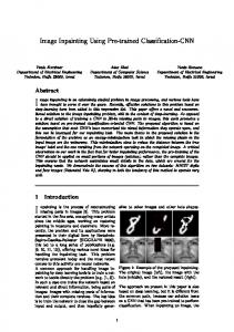
BioMed Research International function neural network (RBFNN) with independent component analysis (ICA) for two-class classification. They achieved an accuracy of 90% on the WBDC data set [24] with 569 images. Recently for two-class classification Dheeba and Abdel-Zaher et al. used Particle Swarm Optimization-based Wavelet Neural Network (PSO-WNN) and deep belief network (DBN) [25], [26], respectively, and achieved significant results on data set of 216 and 690 images. Uppal and Naseem used fusion of discrete cosine transform and discrete wavelet transform features to classify mammograms in 3 classes [27]; they used data in the MIAS database and obtained high accuracy of 96.97% and 98.39%, respectively. Deep learning methods can perform well at the cost of large amount of data set [28–30]. Table 1 summarizes the significant work done so far for the classification of mammogram images. It can be seen that significant results are achieved for two-class classification. However, for three-class (normal, benign, and malignant) classification, there has been little progress because either of the available data sets are small and private or proposed systems have not achieved very promising results. In this paper, we have extended our previous work [31] and propose an improved classification technique for large data sets of mammograms using CNN. The application of classic approaches, for example, using DSIFT features and SVM classifier, on a classic two-class classification for normal and abnormal or a three-class classification (normal, benign, and malignant) using the rotation and scale invariant DSIFT features [32] and a SVM classifier with linear kernel, did not achieve satisfactory performance. Therefore, a threeclass classification study (malignant, benign, and normal) is carried out by using our proposed model. Example images of these classes are shown in Figure 1. Two different approaches, namely, CNN-DW and CNN-CT, are presented in our proposed model. An augmented data set is produced by using mammogram patches. The data set is filtered by contrast enhancement. In the first method enhanced mammogram images are decomposed as its four subbands by means of 2D-DWT, while in the second method discrete curvelet transform (DCT) is used. In both methods DSIFT descriptor is used to extract features for all subbands. Input data matrix containing these subband features of all the mammogram patches is created that is processed as input to convolutional neural network (CNN). A softmax layer and a SVM layer are used to train CNN for classification. A flow chart of the proposed model is given in Figure 2. The main contribution of this paper is the development of a deep learning method based on a large data set of mammogram images. We have shown that the discriminant and descriptive features can perform well with different wavelets, if these are used according to our proposed model in combination with CNN. We also perform classification with SVM via 10-fold cross-validation presenting more unbiased results. The remaining of the paper is organized as follows. Section 2 explains the feature extraction and representation steps in this research. Section 3 describes the CNN based classification model and SVM classification. Section 4 demonstrates the simulation/results and the paper concludes in Section 5.

BioMed Research International

3

Table 1: State-of-the-art diagnostic schemes for the screening mammography classification. Authors Mazurowski et al. [3] Lesniak et al. [4] Wei et al. [5] Abirami et al. [7] Tagliafico et al. [34] Subashini et al. [35] Elter and Halmeyer [8] Deserno et al. [13]

Year Data sources Technique/classifier Classes Number of images Classification accuracy 2011 DDMS Random mutation hill climbing 2 1,852 49%–83% 2011 Private SVM radial Kernel 2 10,397 66%-67% 2011 DDSM SVM radial Kernel 2 2,563 72%–74% 2016 MIAS Wavelet features 2 322 93% 2009 Private Thresholding 4 160 80%–90% 2010 Private SVM radial Kernel 3 43 95% 2008 DDSM Euclidean metric 2 360 86% 2011 IRMA SVM Gaussian Kernel 12 2796 80% Local linear embedding metric 476 80% Tao et al. [6] 2011 Private 2 Curvature scale space 415 75% Private CNN and LDA 196 — Ge et al. [19] 2006 2 MIAS CNN and LDA 216 — FFDM ADN and SVM 739 — Jamieson et al. [21] 2012 2 Ultrasound ADN and SVM 2393 — Arevalo et al. [22] 2015 BCDR-F03 CNN and SVM 2 736 79.9%–86% Mert et al. [23] 2015 WBDC ICA and RBFNN 2 569 90% Dheeba et al. [25] 2015 Private PSOWNN 2 216 93.6% Abdel-Zaher and Eldeib [26] 2015 WBCD DBN 2 690 99.6% Vani et al. [10] 2010 MIAS ELM Jasmine et al. [11] 2009 MIAS Wavelet & ANN 2 322 87% Xu et al. [12] 2008 MLPNN 120 98% Uppal and Naseem [27] 2016 MIAS Fusion of cosine transform 3 322 96.97%

(a) Normal

(b) Benign

(c) Malignant

Figure 1: Sample images of mammogram patches.

2. Feature Extraction and Representation 2.1. Data Augmentation. In deep learning techniques, the NN models need to learn a large number of parameters. The chance of overfitting the training data increases due to the model complexity. Augmentation of data is an upright way to avoid this action [33]. It artificially creates new sample images by applying transformations like flipping, rotation, and many other makeovers to the actual data sample. For every image, artificially we have produced seven new sample images using the combination of 90, 180, and 270 degrees of rotation and

flipping transformations. Thus, the resulting data set contains seven times more images than the original database has. 2.2. Enhancement of Digital Mammograms. Contrast Limited Adaptive Histogram Equalization (CLAHE) method [36] is used to enhance the often degraded contrast in some of mammogram images. The pixel intensity transforms to a value within the display range proportional to the pixel intensity’s rank in the local intensity histogram. CLAHE is a special case of Adaptive Histogram Equalization (AHE) where images are enhanced by a user defined clip level, that

4

BioMed Research International

Softmax classification

2D DWT Image dataset

Augmentation of dataset

Feature extraction

CNN

SVM classification

Contrast enhancement

Curvelet transform

Feature extraction

Softmax classification CNN SVM classification

Figure 2: Flow chart of proposed model.

Downsampling Downsampling f(n)

2

f(n)

2

B

k(n)

2

Bℎ

a

(5) Every block histogram is modified by the following transformation function: 𝑡

𝐴 𝑡 = ∑𝑝𝑡 (𝐴 𝑖 ) ,

(1)

𝑖=0

Image

k(n)

2

f(n) k(n)

2

Bv

2

Bd

Figure 3: Two-dimensional discrete wavelet transform.

where 𝑝𝑡 (𝐴 𝑖 ) is the probability density function of the input patch image grayscale value at 𝑖 and is define as 𝑝𝑡 (𝐴 𝑖 ) =

𝑚𝑖 , 𝑚

(2)

where 𝑚𝑖 is the gray scale value of input pixel 𝑖 and 𝑚 is the total number of pixels in a block. is, height of the local histogram, and thus on the maximum contrast enhancement factor. In this technique, enhancement is done on very small patches, so the overenhancement due to noise or the effect of edge-shadowing is very low as compared to AHE [37]. The CLAHE method was originally developed to reduce the shadow of edges and noise produced in homogeneous areas in medical images [38]. The method has been used for the enhancement of digital mammograms [36–40] and demonstrated good improvements to mammograms visual quality. An input image 𝐼 with dimensions 𝑀 × 𝑁, is divided into small blocks. CLAHE is then used to enhance the contrast of each block. Finally the bilinear interpolation is used to combine the neighboring blocks back into whole images. The steps in CLAHE are described as below [40]. (1) Images patches are divided into nonoverlapping blocks of size 8 × 8. (2) The histogram of each block is calculated. (3) For contrast enhancement of patches, a clip limit of histogram, 𝑡 = 0.001, is set. (4) After clipping the threshold value the histogram is redistributed.

(6) Bilinear interpolation is used to combine the neighboring blocks in each patch. The gray scale value of the patch is also changed according to the new histogram. In our experiment, we have used the block size of 8 × 8 and clip limit of histogram is defined as 0.001. 2.3. Two-Dimensional Discrete Wavelet Transform. A twodimensional DWT consists of downsamplers and digital filter banks. The digital filter banks comprise low pass filter 𝑓(𝑛) and high pass filter 𝑘(𝑛). The number of banks depends upon desired resolution of the application [41]. As the mammogram images are two-dimensional signal, the DWT can be computed by separable wavelet functions. As shown in Figure 3, the columns and rows of the image are distinctly processed over the one-dimensional wavelet transform to establish the two-dimensional DWT. In frequency domain the enhanced image 𝐸 is decomposed into subband images at resolution 2𝑗+1 . 𝐵𝑎 is the approximation of the image. 𝐵𝑑 , 𝐵ℎ , and 𝐵V are three detailed subband images in diagonal, horizontal, and vertical, directions, respectively. As a result of wavelet decomposition the image 𝐼 decomposed into four subband components like High-High (HH), High-Low (HL), Low-High (LH), and Low-Low (LL), which correspond to subimages that are 𝐵𝑎 , 𝐵𝑑 , 𝐵V , and 𝐵ℎ , respectively, as shown in Figure 3.

BioMed Research International

5

2.4. Discrete Curvelet Transform. Discrete curvelet transform is an image representation technique used in computer vision. It was proposed by Candes and Donoho [42]. DCT codes image edges more efficiently than wavelet transform [43] and it has useful geometric features that can be used as a feature vector in medical image processing. Eltoukhy et al. [44, 45] have used DCT for the mammogram images. Let 𝐿 be a function that has a discontinuity across a curve and is smooth otherwise, and consider approximating 𝐿 from the best 𝑛-terms in the expansion. The squared error of such an 𝑛-term expansion obeys [46] 󵄩2 1 󵄩󵄩 󵄩󵄩𝐿 − 𝐿 𝑓̃ 󵄩󵄩󵄩 𝛼 󵄩 √𝑚 , 󵄩

𝑚 󳨀→ +∞,

(3)

where 𝐿 𝑓̃ is the approximation from 𝑛 best Fourier coefficients. Equation (4) shows the expansion for wavelet, 󵄩2 1 󵄩󵄩 󵄩󵄩𝐿 − 𝐿 𝑤̃ 󵄩󵄩󵄩 𝛼 , 𝑚

𝑚 󳨀→ +∞,

(4)

where 𝐿 𝑤̃ is the approximation from 𝑛 best wavelet coefficients. Equation (5) shows the expansion for curvelet expansion, 󵄩2 1 󵄩󵄩 3 󵄩󵄩𝐿 − 𝐿 ̃𝑐󵄩󵄩󵄩 𝛼 2 log (𝑚) , 𝑚

𝑚 󳨀→ +∞,

(5)

where 𝐿 ̃𝑐 is the approximation from the 𝑛 best curvelet coefficients. Equation (5) shows that the MSE will be reduced in DCT. Fast DCT proposed in [47] is described as below. It has a two-dimensional space 𝑅2 with 𝜔 as the frequency domain variable and 𝑥 as the spatial variable, and 𝑟 and 𝜃 are the polar coordinates in the frequency domain. A pair of windows 𝑉(𝑡) and 𝑊(𝑟) are defined, which will be called the angular window and the radial window, respectively. 𝑉 is taking real arguments and supported on 𝑟 ∈ (−1, 1) and 𝑊 is taking positive real arguments and supported on 𝑟 ∈ (1/2, 2). ∞ 3 3 ∑ 𝑤2 (2𝑎 𝑟) = 1, 𝑟 ∈ ( , ) , 2 2 𝑎=−∞ ∞

1 1 ∑ V (𝑡 − 𝑏) = 1, 𝑟 ∈ (− , ) . 2 2 𝑏=−∞

(6)

2

For each 𝑎 ≥ 𝑎0 , a frequency window 𝑈𝑎 is defined as −3𝑎/4

𝑈𝑎 (𝑟, 𝜃) = 2

2(𝜀𝑗/2)𝜃 𝑤 (2 𝑟) V ( ). 2𝜋 −𝑎

(7)

The scaled and shifted curvelet in frequency domain is defined as ̃ 𝑗 (𝑈𝑎 (𝑟 − 𝑘, 𝜃 − 𝜃𝑏 )) . ̃ 𝑎,𝑘,𝑏 (𝑥) = 𝜑 𝜑

(8)

From Plancherel theorem, curvelet coefficients can be computed as 𝐶𝑎,𝑘,𝑏 (𝑥) =

1 ̃ 𝑎 (𝑈𝑎 (𝑟 − 𝑘, 𝜃 − 𝜃𝑏 )) 𝑑𝜔. ∫ 𝑓 (𝜔) 𝜑 (2𝜋)2

(9)

𝐶𝑎,𝑘,𝑏 (𝑥) are curvelet coefficients in 4 subbands of spatial frequencies, namely, 𝐹1, 𝐹2, 𝐹3, and 𝐹4.

2.5. Dense Scale Invariant Feature Transform. In next step DSIFT descriptor is extracted from all the subbands components. Dense SIFT scale-space extrema detection used Difference-of-Gaussian (DOG) function to identify potential interest points [48], which were invariant to scale and orientation. ̃ (𝑥, 𝑦) , (10) 𝐷 (𝑥, 𝑦, 𝜎) = (𝐺 (𝑥, 𝑦, 𝛼𝜎) − 𝐺 (𝑥, 𝑦, 𝜎)) ∗ 𝐸 ̃ is the decomwhere 𝛼 is a constant multiplicative factor, 𝐸 posed subband of enhanced patch 𝐸, and 𝐺(𝑥, 𝑦, 𝜎) represent variable scale Gaussian; that is, 𝐺 (𝑥, 𝑦, 𝜎) =

1 −(𝑥2 +𝑦2 /2𝜎2 ) 𝑒 . 2𝜋𝜎2

(11)

Equation (10) can be written as 𝐷 (𝑥, 𝑦, 𝜎) = 𝐺 (𝑥, 𝑦, 𝛼𝜎) ∗ 𝐼 (𝑥, 𝑦) − 𝐺 (𝑥, 𝑦, 𝜎) ̃ (𝑥, 𝑦) = 𝐿 (𝑥, 𝑦, 𝛼𝜎) − 𝐿 (𝑥, 𝑦, 𝜎) , ∗𝐸

(12)

where the scale space of an image 𝐿(𝑥, 𝑦, 𝛼𝜎) is the convõ 𝑦). DOG is used here lution of 𝐺 with an input image 𝐸(𝑥, instead of Gaussian to improve the computation speed. In the key point localization stage, Hessian matrix is used to compute principal curvatures that eliminate the edges by rejecting the low contrast point [48]. Key point descriptor can be found out by using a three-dimensional histogram in which two dimensions correspond to image spatial dimensions and the third dimension corresponds to the image gradient direction computed centered at the key points. The DSIFT descriptor is applied to all the subbands with step size 4 and radius size 5. Feature matrices having dimension (128 × 400) are extracted for all the subbands. From the columns of this matrix, six time domain features, kurtosis, mean, skewness, energy, maximum, and standard deviation, are extracted for each subband. The resultant feature matrix is of the shape of (128 × 6). This matrix is reshaped into a vector form of (1 × 768). Weighting coefficients are applied to the subband images according to (13) and (14) for CNN-DW and CNN-CT method, respectively. Feature vector = (3 ∗ LL + 2 ∗ LH + 2 ∗ HL) ,

(13)

Feature vector = (𝐹1 + 3 ∗ 𝐹2 + 2 ∗ 𝐹3 + 2 ∗ 𝐹4) .

(14)

Equal zero padding is performed on the start and end columns such that it reshapes as (1 × 785). Enhancement and feature extraction steps are performed on all the augmented ̃ 𝑦) of the shape data sets so that we have a data matrix 𝑀(𝑥, (22368 × 785), where 22368 is the number of the sample images and 784 is the number of features of each sample, and every sample has a last column label that belongs to its receptive patch class.

3. Convolution Neural Network In the next step we use CNN to learn features from the data ̃ CNN has proved its importance in classification set matrix 𝑀.

6

BioMed Research International Convolution layer

Input image 28 × 28

Pooling layer

16 @ 7 × 7

Convolution layer

2×2

Pooling layer

Fully connected layer

2×2

16 @ 5 × 5

3-output classification

Figure 4: Convolution neural network model.

of images by its significance results. CNN has a multilayered architecture, consisting of a convolution layer followed by a maximum pooling layer. The number of layers depends upon the designer. The output of final maximum pooling layer is fed to a fully connected layer that works like MLP which is further forwarded to softmax layer. The convolution layer takes 1D or 2D matrices as an input. Equation (15) shows the single output matrix of convolution layer. 𝑁

̃ 𝑖 ∗ 𝐿 𝑖,𝑗 + 𝜌𝑗 ) , 𝐶𝑗 = 𝑓 (∑𝑀

(15)

𝑖=1

̃ 𝑖 is the input matrix that convolves with kernel where 𝑀 matrices 𝐿 𝑖,𝑗 . Bias 𝜌𝑗 is added to each element of output after computing the sum of all convoluted matrices. 𝐶𝑗 is the one output matrix computed by a nonlinear activation function 𝑓, that is applied to each element. Commonly used activation functions in convolution layer are tangent hyperbolic function and sigmoid function as follows: 𝑓 (𝑥) =

1 , 1 + exp (−𝑥)

also use SVM layer instead of the softmax layer. All the other settings of the process remain the same as explained above. SVMs have been applied to many classification tasks [50, 51]. Input data 𝑥 is labeled as 𝑦 = −1 for class 1 and as 𝑦 = 1 for class 2. For linearly separable data a hyperplane can be defined as 𝑛

𝑔 (𝑥) = 𝑤𝑇 𝑥 + 𝑏 = ∑𝑤𝑖𝑇 𝑥𝑖 + 𝑏,

(17)

𝑖=1

where 𝑥 is the input vector, 𝑏 is a scalar, and 𝑤 is 𝑛 dimensional normal vector of this hyperplane. Distance from origin perpendicular to this plane is −𝑏/‖𝑤‖. The solution of SVM is based on optimal hyperplane and minimum mean square error that is defined as 𝐸 (𝑤, 𝑏) =

𝑚 1 2 ‖𝑤‖2 − ∑𝜆 𝑖 (𝑦𝑖 − 𝑔 (𝑥𝑖 )) , 2 𝑖=1

(18)

where 𝜆 is a Lagrangian coefficient and 𝜆 𝑖 > 0. Maximizing (18) results, 𝑚

𝑤 = ∑𝜆 𝑖 𝑦𝑖 𝑥𝑖 ,

(16)

𝑓 (𝑥) = tanh (𝑥) . The pooling layer is used for dimensionality reduction in the convolution layer. Mostly used pooling layer algorithms are average pooling, mean pooling, and maximum pooling. During the training, the dropout algorithm is applied by randomly disabling the neurons, with a normally dropout ratio between 0.3 and 0.6. The final layer of CNN is a soft max layer that contains the output neuron according to the number of classes of the problem, which is assigned a confidence score. The overall network design of CNN is presented in Figure 4. The two convolutional and max pooling layers are used with a kernel size of 2 × 2. Convolutional layers have 16 kernels with size of 7 × 7 and the second layer uses kernel sized 5 × 5. Then, a fully connected neural layer is used. The dropout ratio in the experiment is 0.55. Softmax layer is used to train CNN for classification. 3.1. Classification with Support Vector Machines. Recently, many researchers have used SVM as a top layer instead of softmax layer in deep learning and showed improvements in the classification result [49]. In the second experiment we

𝑖=1

𝑚

(19)

∑𝜆 𝑖 𝑦𝑖 = 0. 𝑖=1

Putting (19) into (18), it is redefined as 𝑚 1𝑚 𝑚 ] (𝜆) = ∑𝜆 𝑖 − ∑ ∑ 𝜆 𝑖 𝜆 𝑗 𝑦𝑖 𝑦𝑗 𝐾 (𝑥𝑖 𝑥𝑗 ) , 2 𝑖=1 𝑗=1 𝑖=1

(20)

where 𝐾(𝑥𝑖 𝑥𝑗 ) is the kernel function [52].

4. Simulation and Results This section presents the database and validation assessment measures that are used in this experiment. Moreover, the experimental results are presented to show the superiority of proposed methods. 4.1. Database. We have used IRMA data set [53] for experiments in this study. A total of 2796 patches of the original mammogram images are used for this experiment. Selected IRMA patches consist of four different sources including 2,576 images from DDSM, 150 images from MIAS,

BioMed Research International

7

90

60

83.2

57.54 51.4

80 74.6

75 70 65 60

56.83

82.26 Accuracy rate

Accuracy rate

85

70

50 40 30 20 10

HOG

LCP

0

DSIFT

HOG

LCP

DSIFT

Figure 5: Comparison of two-class classification accuracy rate for HOG LCP and DSIFT.

Figure 6: Comparison of three-class classification accuracy rate for HOG LCP and DSIFT.

and Lawrence Livermore National Laboratory (LLNL) and Rheinisch Westf¨alische Technische Hochschule (RWTH) contribute 1 and 69 images, respectively. The selected images are further divided into three classes, malignant, benign, and normal, as prescribed in IRMA data set. The final size of mammogram images patches is 128 × 128 pixels.

Unlike sensitivity, specificity deals only with negative cases. It is the ratio of the detected true negative over the actual negative.

4.2. Validity Assessment Measures. The validation of the method is measured by classification accuracy, Positive Predictive Value (PPV), Negative Predictive Value (NPV), sensitivity, specificity, Matthews Correlation Coefficient (MCC), and Receiver Operating Characteristic (ROC). In medical image classification, false positive (FP) is the incorrect classification rate of samples, such that a disease result is positive, when in reality it is not, while false negative (FN) is the incorrect classification rate of samples, in which a test result improperly indicates no presence of a condition. True positive (TP) is the correct classification rate of positive samples, while true negative is the correct classification rate of negative samples. Accuracy is the most commonly used assessment measure for classification that considers all the cases; it used all the cases. Accuracy =

TN + TP . FP + FN + TP + TN

(21)

PPV is defined as the number of the correct detected positive cases over all detected positive cases. PPV =

TP . FP + TP

(22)

NPV is defined as the number of the true negative cases detected over all negative cases. NPV =

TN . FN + TN

(23)

Sensitivity is defined as the ratio of the detected true positive cases over actual positive cases. It deals only with positive cases. Sensitivity =

TP . FN + TP

(24)

Specificity =

TN . FP + TN

(25)

MCC is an assessment indicator of deep learning methods, particularly for the negative case sample detected, that are evidently unbalanced compared with the positive sample detected. MCC provides a superior assessment compared to the general accuracy. MCC =

(26) TP × TN − FP × FN . √(TP + FP) (TP + FN) (TN + FP) (TN + FN)

The ROC curve is used for measuring the predictive accuracy of the model. It indicates the relation between the true positive rate and false positive rate. 4.3. Experimental Results. In this subsection the proposed methods have been compared with existing methods in terms of accuracy rate, error rate, and various validation assessment measures. Figure 5 shows the result of two-class classification. It can be observed that in two-class classification Histogram Oriented Gradient (HOG) method performs better with an accuracy rate of 83.2%. The other two schemes, Local Configuration Pattern (LCP) and DSIFT, have accuracy rates of 82.26% and 74.6%, respectively. Likewise, Figure 6 shows the result of three-class classification. Here LCP method performs better than the other two schemes with the best accuracy of 57.54, but the results are not so promising. This accuracy has been further enhanced by our methods as shown in the rest of the simulation results. In Figure 7, the accuracy rate of proposed CNN-DW method has been presented for different number of iterations using softmax layer. Note that the classification results for three-class category obtained by proposed CNN-DW method are more pleasing as compared to the existing schemes in Figure 6. CNN-DW method achieved the accuracy of 83.14% and 81.18% on validation data set and test data set, respectively. Furthermore, Figure 8 shows the error rate of the

84 82.76 83.14 83 82.27 81.83 82 81.21 81.35 81.05 81.18 80.61 81 80.17 80 79.12 79.29 79.42 79 77.77 78 77 76 75 600 100 200 300 400 500 700

Accuracy rate

BioMed Research International

Accuracy rate

8

84.51 85 84.57 84.15 83.71 83.46 84 83.01 82.46 82.54 83 81.85 82.19 82 81.33 81.08 81 80.43 79.88 80 79 78 77 100 200 300 400 500 600 700

Iterations

Iterations Valid Test

Valid Test

Figure 7: Accuracy rate of proposed CNN-DW method for test and validation data sets.

Figure 9: Accuracy rate of proposed CNN-CT method for test and validation data sets. 22

23

21

22

20 Error rate

Error rate

21 20 19

18 17

18

16

17 16

19

15 100

200

300

400 500 Iterations

600

700

Valid Test

Figure 8: Error rate of proposed CNN-DW method for test and validation data sets.

proposed CNN-DW method with softmax layer at different iterations. With softmax layer, it has 16.86 and 18.82 error on validation data set and test data set, respectively. Likewise, the accuracy rate and error rate of second proposed method, that is, CNN-CT, have been shown. Figure 9 shows the accuracy rate of proposed CNN-CT method with softmax layer at different iterations. Note that the classification results for three-class category obtained by proposed CNN-CT method are better as compared to the existing schemes in Figure 6 and from CNN-DW method as well. The proposed method achieved the accuracy of 84.57% and 82.54% on validation data set and test data set, respectively. Similarly, Figure 10 shows the error rate of proposed CNN-CT method with softmax layer at different iterations. With softmax layer, it has 15.43 and 17.46 error on validation data set and test data set, respectively. In the further simulation, the results of our proposed methods using SVM layer are presented. Figure 11 shows the accuracy rate of proposed CNN-DW method with SVM layer at different instants. It is shown that proposed CNN-DW method has achieved an average accuracy of 81.83%. Likewise, Figure 13 shows the accuracy rate of the other proposed CNN-CT method with SVM layer. Proposed curvelet method has achieved average accuracy of 83.74%.

100

200

300

400 500 Iterations

600

700

Valid Test

Figure 10: Error rate of proposed CNN-CT method for test and validation data sets.

Moreover, the proposed methods are also tested for SVM 10-fold cross-validation. Figure 12 shows the accuracy rate of proposed CNN-DW method with SVM layer and it has achieved average accuracy of 81.23% in 10-fold crossvalidation. Similarly, Figure 14 shows the accuracy rate of proposed CNN-CT method with 10-fold cross-validated SVM layer. It has achieved an average accuracy of 83.11%. Table 2 shows the quantitative comparison of existing and proposed schemes. It can easily be observed that the proposed CNN-DW and CNN-CT methods provide better measure values, especially on large data set of mammogram images. Proposed CNN WT method has outperforms all other methods. Similarly, Table 3 shows the quantitative comparison for SVM classifier with 10-fold cross-validation of the existing and proposed schemes. It can easily be observed that the proposed scheme provides better measure values in both the cases. Finally, Table 4 provides a summary on accuracy rate for 3-class classification.

5. Conclusion A novel mammograms classification method for breast cancer detection based on CNN is proposed. We have proposed two algorithms; first algorithm is based on 2D discrete

BioMed Research International

9 Table 2: Validity assessment measures for SVM classifier.

PPV 0.698 0.701 0.484 0.853 0.881

HOG LCP DSIFT Proposed CNN-WT Proposed CNN-CT

NPV 0.890 0.911 0.851 0.921 0.939

Sensitivity 0.838 0.816 0.808 0.876 0.888

Specificity 0.710 0.762 0.682 0.819 0.801

MCC .671 .701 .629 .816 .829

ROC .729 .746 .684 .846 .855

MCC .641 .675 .589 .802 .810

ROC .687 .712 .651 .831 .839

Table 3: Validity assessment measures for SVM classifier with 10-fold cross-validation. PPV 0.654 0.663 0.441 0.818 0.839

HOG LCP DSIFT Proposed CNN-WT Proposed CNN-CT

NPV 0.847 0.881 0.824 0.891 0.904

Sensitivity 0.803 0.769 0.776 0.833 0.854

90

88 85.82

88 84.04

84

83.63 83.27

81.56

82

82.56 81.14

79.79

80

79.00 77.58

78 76

Accuracy rate

Accuracy rate

86

1

2

3

4

5

6

7

8

9

82.65

83.70

84.75

81.65

79.26

80 78

72

10

Figure 11: Accuracy rate of proposed CNN-DW method with SVM classifier. 90

86.83

85.77

80 77.3

81.23 81.49

79.79 80.14

Accuracy rate

81.21

75.09 75 70

1

2

3

4

5

6

7

8

9

10

Cross fold

1

2

3

4

5 6 Instants

7

8

9

10

Figure 13: Accuracy rate of proposed CNN-CT method with SVM classifier.

83.63

85 Accuracy rate

86.96 84.91

74

Instant

65

85.91

86 84.96 84 82.71 82

76

74 72

Specificity 0.671 0.737 0.642 0.782 0.797

90 88 86.83 85.77 86 84.79 83.47 83.41 83.21 84 82.64 82.14 82 79.96 78.89 80 78 76 74 72 1 2 3 4 5 6 7 8 9 10 Cross fold

Figure 12: Accuracy rate of proposed CNN-DW method with SVM using 10-fold cross-validation.

Figure 14: Accuracy rate of proposed CNN-CT method with SVM using 10-fold cross-validation.

wavelet transform while the other is based on curvelet transform. We have found that deep learning method can be used for the breast cancer detection by using data augmentation and results show that learning features from the data set before inputting the data to the CNN is more helpful for cancer detection. We have also found that by using the SVM layer instead of softmax layer the classification performance

can be improved. However, the 10-fold cross-validated result of the SVM can cut down the accuracy because the crossvalidated result is more unbiased than performing training and testing process proposed method with curvelet transform has better results as compared to the proposed method with wavelet method and other existing methods. In future work, more techniques of deep learning can be applied for the

10

BioMed Research International Table 4: Summarized accuracy rate for 3-class classification on large data set.

SVM layer SVM 10-fold cross-validation Softmax layer

HOG 56.83 56.27 —

LCP 57.54 57.13 —

detection of breast cancer. Improvement can also be made by using different architecture of CNN.

Competing Interests The authors declare that there is no conflict of interests regarding the publication of this paper.

Acknowledgments The authors would like to thank IRMA group, Aachen, Germany, for sharing their data set with them for this experimental study.

References [1] https://www.breastcancercare.org.uk/about-us/media/press-pack -breast-cancer-awareness-month/facts-statistics. [2] American Cancer Society, http://www.cancer.org/cancer/breastcancer/detailedguide/breast-cancer-detection. [3] M. A. Mazurowski, J. Y. Lo, B. P. Harrawood, and G. D. Tourassi, “Mutual information-based template matching scheme for detection of breast masses: from mammography to digital breast tomosynthesis,” Journal of Biomedical Informatics, vol. 44, no. 5, pp. 815–823, 2011. [4] J. Lesniak, R. Hupse, M. Kallenberg et al., “Computer aided detection of breast masses in mammography using support vector machine classification,” in Proceedings of the Medical Imaging 2011: Computer-Aided Diagnosis, 2011. [5] C.-H. Wei, Y. Li, and P. J. Huang, “Mammogram retrieval through machine learning within BI-RADS standards,” Journal of Biomedical Informatics, vol. 44, no. 4, pp. 607–614, 2011. [6] Y. Tao, S. C. B. Lo, L. Hadjiski, H. P. Chan, and T. M. Freedman, “Birads guided mammographic mass retrieval,” in Proceedings of the Medical imaging, Proceedings of SPIE, 2011. [7] C. Abirami, R. Harikumar, and S. Chakravarthy, “Performance analysis and detection of micro calcification in digital mammograms using wavelet features,” in Proceedings of the International Conference on Wireless Communications, Signal Processing and Networking (WiSPNET ’16), pp. 2327–2331, Chennai, India, March 2016. [8] M. Elter and E. Halmeyer, “A knowledge-based approach to the CADx of mammographic masses,” in Proceedings of the Medical Imaging 2008: Computer-Aided Diagnosis, vol. 6915 of Proceedings of SPIE, San Diego, Calif, USA, February 2008. [9] J. Suckling, “The mammographic image analysis society digital mammogram database,” Exerpta Medica. International Congress Series, vol. 1069, pp. 375–378, 1994. [10] G. Vani, R. Savitha, and N. Sundararajan, “Classification of abnormalities in digitized mammograms using extreme learning machine,” in Proceedings of the 11th International Conference on Control, Automation, Robotics and Vision (ICARCV ’10), pp. 2114–2117, IEEE, Singapore, December 2010.

DSIFT 51.40 50.91 —

CNN-WT 81.83 81.24 79.92

CNN-CT 83.74 83.11 81.49

[11] J. A. Jasmine, A. Govardhan, and S. Baskaran, “Microcalcification detection in digital mammograms based on wavelet analysis and neural networks,” in Proceedings of the International Conference on Control, Automation, Communication and Energy Conservation (INCACEC ’09), pp. 1–6, Perundurai, India, June 2009. [12] W. Xu, W. Liu, L. Li, G. Shao, and J. Zhang, “Identification of masses and microcalcifications in the mammograms based on three neural networks: comparison and discussion,” in Proceedings of the 2nd International Conference on Bioinformatics and Biomedical Engineering (iCBBE ’08), pp. 2299–2302, May 2008. [13] T. M. Deserno, M. Soiron, J. E. E. de Oliveira, and A. A. de Ara´ujo, “Towards computer-aided diagnostics of screening mammography using content-based image retrieval,” in Proceedings of the 24th SIBGRAPI Conference on Graphics, Patterns and Images, pp. 211–219, Macei´o, Brazil, August 2011. [14] Y. Bengio, A. Courville, and P. Vincent, “Representation learning: a review and new perspectives,” IEEE Transactions on Pattern Analysis and Machine Intelligence, vol. 35, no. 8, pp. 1798–1828, 2013. [15] J. Arevalo, A. Cruz-Roa, and F. A. Gonzlez, “Hybrid image representation learning model with invariant features for basal cell carcinoma detection,” 2013. [16] A. Jalalian, S. B. T. Mashohor, H. R. Mahmud, M. I. B. Saripan, A. R. B. Ramli, and B. Karasfi, “Computer-aided detection/diagnosis of breast cancer in mammography and ultrasound: a review,” Clinical Imaging, vol. 37, no. 3, pp. 420– 426, 2013. [17] K. Petersen, M. Nielsen, P. Diao, N. Karssemeijer, and M. Lillholm, “Breast tissue segmentation and mammographic risk scoring using deep learning,” in Breast Imaging: 12th International Workshop, IWDM 2014, Gifu City, Japan, June 29–July 2, 2014. Proceedings, vol. 8539 of Lecture Notes in Computer Science, pp. 88–94, Springer, Berlin, Germany, 2014. [18] K. Petersen, K. Chernoff, M. Nielsen, and A. Y. Ng, “Breast density scoring with multiscale denoising autoencoders,” in Proceedings of the STMI Workshop at the 15th International Conference on Medical Image Computing and Computer Assisted Intervention (MICCAI ’12), Nice, France, 2012. [19] J. Ge, B. Sahiner, L. M. Hadjiiski et al., “Computer aided detection of clusters of microcalcifications on full field digital mammograms,” Medical Physics, vol. 33, no. 8, pp. 2975–2988, 2006. [20] M. Kallenberg, K. Petersen, M. Nielsen et al., “Unsupervised deep learning applied to breast density segmentation and mammographic risk scoring,” IEEE Transactions on Medical Imaging, vol. 35, no. 5, pp. 1322–1331, 2016. [21] A. R. Jamieson, K. Drukker, and M. L. Giger, “Breast image feature learning with adaptive deconvolutional networks,” in Proceedings of the Medical Imaging 2012: Computer-Aided Diagnosis, Proceedings of SPIE, San Diego, Calif, USA, February 2012. [22] J. Arevalo, F. A. Gonzalez, R. Ramos-Pollan, J. L. Oliveira, and M. A. Guevara Lopez, “Convolutional neural networks for

BioMed Research International

[23]

[24] [25]

[26]

[27]

[28]

[29]

[30]

[31]

[32]

[33]

[34]

[35]

[36]

[37]

[38]

[39]

mammography mass lesion classification,” in Proceedings of the Engineering in Medicine and Biology Society (EMBC ’15), vol. 25, pp. 797–800, August 2015. A. Mert, N. Kılıc¸, E. Bilgili, and A. Akan, “Breast cancer detection with reduced feature set,” Computational and Mathematical Methods in Medicine, vol. 2015, Article ID 265138, 11 pages, 2015. https://archive.ics.uci.edu/ml/datasets. J. Dheeba, N. Albert Singh, and S. Tamil Selvi, “Computer-aided detection of breast cancer on mammograms: a swarm intelligence optimized wavelet neural network approach,” Journal of Biomedical Informatics, vol. 49, pp. 45–52, 2014. A. M. Abdel-Zaher and A. M. Eldeib, “Breast cancer classification using deep belief networks,” Expert Systems with Applications, vol. 46, pp. 139–144, 2016. Uppal and M. T. Naseem, “Classification of mammograms for breast cancer detection using fusion of discrete cosine transform and discrete wavelet transform features,” Biomedical Research, In press. A. Krizhevsky, I. Sutskever, and G. E. Hinton, “Imagenet classification with deep convolutional neural networks,” in Advances in Neural Information Processing Systems, pp. 1097–1105, MIT Press, 2012. D. Ciresan, U. Meier, and J. Schmidhuber, “Multi-column deep neural networks for image classification,” in Proceedings of the IEEE Conference on Computer Vision and Pattern Recognition (CVPR ’12), pp. 3642–3649, Providence, RI, USA, June 2012. D. C. Ciresan, U. Meier, J. Masci, L. M. Gambardella, and J. Schmidhuber, “High-performance neural networks for visual object classification,” https://arxiv.org/abs/1102.0183. M. Mohsin Khan, Q. Zhang, S. Butt, and I. Ul Haq, “Novel mammograms classification for breast cancer detection based on multi-layer perceptron,” in Proceedings of the 4th International Conference Advances in Computing, Communication and Information Technology (CCIT ’16), Birmingham, UK, 2016. D. G. Lowe, “Distinctive image features from scale-invariant keypoints,” International Journal of Computer Vision, vol. 60, no. 2, pp. 91–110, 2004. A. Krizhevsky, I. Sutskever, and G. E. Hinton, “Imagenet classification with deep convolutional neural networks,” in Advances in Neural Information Processing Systems, pp. 1097–1105, 2012. A. Tagliafico, G. Tagliafico, S. Tosto et al., “Mammographic density estimation: comparison among BI-RADS categories, a semi-automated software and a fully automated one,” The Breast, vol. 18, no. 1, pp. 35–40, 2009. T. S. Subashini, V. Ramalingam, and S. Palanivel, “Automated assessment of breast tissue density in digital mammograms,” Computer Vision and Image Understanding, vol. 114, no. 1, pp. 33–43, 2010. S. M. Pizer, “Psychovisual issues in the display of medical images,” in Pictoral Information Systems in Medicine, K. H. Hoehne, Ed., pp. 211–234, Springer, Berlin, Germany, 1985. E. D. Pisano, S. Zong, B. M. Hemminger et al., “Contrast limited adaptive histogram equalization image processing to improve the detection of simulated spiculations in dense mammograms,” Journal of Digital Imaging, vol. 11, no. 4, pp. 193–200, 1998. X. Wang, B. S. Wong, and T. C. Guan, “Image enhancement for radiography inspection,” in Proceedings of the SPIE Proceedings, pp. 462–468, Singapore, 2004. J. E. Ball and L. M. Bruce, “Digital mammogram spiculated mass detection and spicule segmentation using level sets,” in

11

[40]

[41] [42]

[43] [44]

[45]

[46] [47]

[48]

[49] [50]

[51]

[52]

[53]

Proceedings of the 29th Annual International Conference of IEEEEMBS, Engineering in Medicine and Biology Society (EMBC ’07), pp. 4979–4984, Lyon, France, August 2007. I. K. Maitra, S. Nag, and S. K. Bandyopadhyay, “Technique for preprocessing of digital mammogram,” Computer Methods and Programs in Biomedicine, vol. 107, no. 2, pp. 175–188, 2012. S. Mallat, A Wavelet Tour of Signal Processing, Academic Press, 1999. E. Candes and D. Donoho, “Curvelets, multiresolution representation, and scaling laws,” in Wavelet Applications in Signal and Image Processing VIII, A. Aldroubi, A. F. Laine, and M. A. Unser, Eds., vol. 4119 of Proceedings of SPIE, December 2000. K. P. Soman and K. I. Ramachandran, Insight into Wavelets: From Theory to Practice, Prentice-Hall Press, 2nd edition, 2006. M. M. Eltoukhy, I. Faye, and B. Belhaouari Samir, “A comparison of wavelet and curvelet for breast cancer diagnosis in digital mammogram,” Computers in Biology and Medicine, vol. 40, no. 4, pp. 384–391, 2010. M. M. Eltoukhy, I. Faye, and B. B. Samir, “Breast cancer diagnosis in digital mammogram using multiscale curvelet transform,” Computerized Medical Imaging and Graphics, vol. 34, no. 4, pp. 269–276, 2010. K. P. Soman and K. I. Ramachandran, Insight into Wavelets: From Theory to Practice, Prentice-Hall, 2nd edition, 2006. E. Cand`es, L. Demanet, D. Donoho, and L. Ying, “Fast discrete curvelet transforms,” Multiscale Modeling and Simulation, vol. 5, no. 3, pp. 861–899, 2006. D. G. Lowe, “Distinctive image features from scale-invariant keypoints,” International Journal of Computer Vision, vol. 60, no. 2, pp. 91–110, 2004. Y. Tang, “Deep learning using linear support vector machines,” https://arxiv.org/abs/1306.0239. V. N. Vapnik, Statistical learning theory, Adaptive and Learning Systems for Signal Processing, Communications, and Control, John Wiley & Sons, Inc., New York, USA, 1998. C. J. C. Burges, “A tutorial on support vector machines for pattern recognition,” Data Mining and Knowledge Discovery, vol. 2, no. 2, pp. 121–167, 1998. A. Wang, W. Yuan, J. Liu, Z. Yu, and H. Li, “A novel pattern recognition algorithm: combining ART network with SVM to reconstruct a multi-class classifier,” Computers and Mathematics with Applications, vol. 57, no. 11-12, pp. 1908–1914, 2009. J. E. E. Oliveira, M. O. Gueld, A. D. A. Ara´ujo, B. Ott, and T. M. Deserno, “Towards a standard reference database for computeraided mammography,” in Proceedings of the Medical Imaging 2008—Computer-Aided Diagnosis, Proceedings of SPIE, San Diego, Calif, USA, February 2008.

MEDIATORS of

INFLAMMATION

The Scientific World Journal Hindawi Publishing Corporation http://www.hindawi.com

Volume 2014

Gastroenterology Research and Practice Hindawi Publishing Corporation http://www.hindawi.com

Volume 2014

Journal of

Hindawi Publishing Corporation http://www.hindawi.com

Diabetes Research Volume 2014

Hindawi Publishing Corporation http://www.hindawi.com

Volume 2014

Hindawi Publishing Corporation http://www.hindawi.com

Volume 2014

International Journal of

Journal of

Endocrinology

Immunology Research Hindawi Publishing Corporation http://www.hindawi.com

Disease Markers

Hindawi Publishing Corporation http://www.hindawi.com

Volume 2014

Volume 2014

Submit your manuscripts at https://www.hindawi.com BioMed Research International

PPAR Research Hindawi Publishing Corporation http://www.hindawi.com

Hindawi Publishing Corporation http://www.hindawi.com

Volume 2014

Volume 2014

Journal of

Obesity

Journal of

Ophthalmology Hindawi Publishing Corporation http://www.hindawi.com

Volume 2014

Evidence-Based Complementary and Alternative Medicine

Stem Cells International Hindawi Publishing Corporation http://www.hindawi.com

Volume 2014

Hindawi Publishing Corporation http://www.hindawi.com

Volume 2014

Journal of

Oncology Hindawi Publishing Corporation http://www.hindawi.com

Volume 2014

Hindawi Publishing Corporation http://www.hindawi.com

Volume 2014

Parkinson’s Disease

Computational and Mathematical Methods in Medicine Hindawi Publishing Corporation http://www.hindawi.com

Volume 2014

AIDS

Behavioural Neurology Hindawi Publishing Corporation http://www.hindawi.com

Research and Treatment Volume 2014

Hindawi Publishing Corporation http://www.hindawi.com

Volume 2014

Hindawi Publishing Corporation http://www.hindawi.com

Volume 2014

Oxidative Medicine and Cellular Longevity Hindawi Publishing Corporation http://www.hindawi.com

Volume 2014