F - Zro is the projection of the point source on the detector plane (see. Figure 4). 3. ITERATIVE ALGORITHMS. The geometric response function is not three-.
IEEE TRANSACTIONS ON NUCLEAR SCIENCE, VOL. 38, NO. 2, APRIL 1991
693
THREE-DIMENSIONAL ITERATIVE RECONSTRUCTION ALGORITHMS WITH ATTENUATION AND GEOMETRIC POINT RESPONSE CORRECTION G. L. Zeng and G. T.Gullberg, Department of Radiology, University of Utah, Salt Lake City, Utah 84132
B. M. W. Tsui and J. A. Terry, Department of Radiology and Cumculum in Biomedical Engineering, University of North Carolina, Chapel Hill, North Carolina 27514 Abstract The point response resolution of a gamma camera deteriorates with increased distance from the face of the collimator. This results in reconstruction artifacts that are seen as shape distortion and density non-uniformity. For parallel, fan, and cone beam geometries, iterative reconstruction algorithms have been developed which eliminate these artifacts by incorporating the three-dimensional spatially varying geometric point response into models for the projection and backprojection operations which also model photon attenuation. The algorithms have been tested on an IBM 3090600s supercomputer. The iterative EM reconstruction algorithm is 50 times longer with geometric response and photon attenuation models than without modeling these physical effects. We have demonstrated an improvement in image quality in the reconstruction of projection data collected from a single photon emission computed tomography (SPECT) imaging system. Using phantom experiments, we observe that the modeling of the spatial system response imposes a smoothing without loss of resolution.
1. INTRODUCTION The point response function of a single photon emission computed tomography (SPECT) system is spatially varying and deteriorates with distance from the face of the collimator. This results in shape distortions and nonuniform density variations in the images reconstructed from projection data obtained from a SPECT imaging system. This problem was recognized early on by Kuhl [l] who in his backprojection tomograms attempted to de-emphasize the effect of the point response deterioration, by performing half backprojections (i.e., backprojecting only half way through the image array). The half backprojection idea was later implemented using the filter backprojection algorithm [2]. This was later modified so that the backprojected value was weighted more for pixels close to the detector and less as pixels are further away [3,4]. Other work has attempted to deconvolve the point response from projection data using variations of Weiner filtering where the MTF is approximated for a point source located at the center of rotation [5]. However, since the geometric response is spatially varying, the most accurate approach, yet computationallytime consuming, is to model the spatially varying geometric point response and to solve the reconstruction problem by determining the solution to a large system of linear equations. Initial work solving a linear system of equations using iterative reconstruction algorithms has been reported where, in the reconstruction of transaxial slices from parallel projections,
the geometric point response variation was modeled as a two dimensional point response function [6-lo]. Here we extend that work to incorporate the three-dimensional response function in reconstructing the three-dimensional volume for parallel, fan beam, and cone beam collimators. In our work an iterative EM algorithm [ l l ] is used to reconstruct the projections. The three-dimensional geometric point response and photon attenuation are incorporated into ray-driven projector-backprojectorsused by the algorithm. An “inversecone” of rays is used in ray-driven projector-backprojectors to model the spread of the geometric detector response function with increased distance from the detector face. We show that the ray-driven projector-backprojector intrinsically models the sensitivity such that geometric response can be weighted by a constant factor along each ray emanating from the detector bin. The over-all point response is a function of attenuation, the source scattering response, the collimator geometric response, septa penetration response, and the intrinsic crystal resolution. In our work here, we neglect the collimator septa penetration and crystal scattering, because they are relatively insignificant compared with the patient-scattering and the system gcometric response. Even though we develop the structure that can also include the scatter response, we do not include it in the work presented here, but we await studies that can better characterize the response function for distributed sources in an attenuating medium [12]. Here we use analytical expressions for the collimator geometric response function that have been derived for parallel [13,14], fan [15], and cone beam [15]collimators and calculate attenuation factors by integrating the known distribution of attenuation coefficients along the cone of rays that emanate from each detector bin using a method first described in [ 161. In this paper, we first present analytical expressions for the geomctric point response for parallel, fan beam, and cone beam geomctries. Then we show how they are incorporated into the ray-driven projector-backprojectors that use an “inversecone” structure of rays that emanate from each projection bin. It is shown that the “inverse-cone” structure is a logical way to model sensitivity,geometric point response, and to calculatethe photon attenuation factors. We also present results of computer simulations for elliptical detector orbits and results of phantom experiments.
2. GEOMETRIC POINT RESPONSE FUNCTIONS The geometric point response function is the photon
0018-9499/91/0400-0693$01.00 0 1991 IEEE
694
fluence distribution on the detector face determined by the geometrical aperture of the collimator holes. The geometric point response assumes no scatter, no septal penetration, and no intrinsic crystal spreading. It depends upon the point source location and the collimator geometry. The geometric point response can be derived by considering one collimator hole. For a point source in Figure 1, we can give an expression for the geometric point response in terms of the autocorrelation of the collimator aperture function a for one collimator hole on the front plane of the collimator [14,15]. The aperture function is considered to have the value 1 for any point inside the aperture and 0 outside. For a point source located at a distance Z from the detector plane, it has been shown [14,15] that the total photon fluence at a point r on the detection plane is prOpOl6OMl to =
j j a (0)a ( 0 +'TI
For a circular hole aperture a(a) with radius R, the integral in (1) can be evaluated by computing the common area of two circles. As shown in Figure 1 this common area is given by the following formula:
$ ( r T ) = R 2 ( O - sine),
(2)
where
00
Q (rT)
Hexagonal hole collimators are commonly used in nuclear medicine applications because of better efficiency compared with other hole shapes. However, it can be shown that the geometric point response function for a hexagonal hole is approximately equal to that of a circular hole collimator. Throughout the development in this paper, we assume that the collimator aperture function U is circular. This assumption simplifies the code and increases computer efficiency.
do
e
(1)
I
= 2 cos-l- r7i
where r, is a function of r, ro the perpendicular projection of the point source on the detection plane, and Z. Expressions for the variable r, which depends upon the collimator geometry are developed in the following sections. Both CJ and rT are on the 6plane, which is obtained through a coordinate transformation from the r-plane [151.
-+t'
(3)
2R '
-0
for 0 I lrd < 2R and zero otherwise. Substituting 8 into (2) gives the following expression
Here we drop the factor R2 and replace it by a normalization factor c, such that
focal point
t
From (4) we see that the geometric point response function Q is dependent upon rT and the hole radius R. In the following sections, rT is given for parallel, fan beam, and cone beam geometries.
2.1. Parallel Ream Geometry Figure 2 illustrates the geometry for a parallel hole collimator. The distance between the collimator backplane and the image plane in the scintillation crystal is represented by B. The thickness of the collimator (the length of the collimator holes) is denoted by L. It can be shown [14] that for parallel beam geometry the parameter r, in (4) is given by
. .. . . . :
....... Point
Source
.......... ........................
1
~
.................. ............
.......
i
.........
Collimator
b Figure 1. Function Q as the common area of two circles.
7
L
Figure 2. Parallel beam geometry.
Plane
695
L rT = z ( r - r o ) . From (6), one observes that @ is shift invariant for any fixed Z. 2.2. Fan Beam Geometry
A fan beam collimator shown in Figure 3 consists of rows of holes that are parallel in the direction of the axis of rotation. In each row, the holes are tapered and are focused to a point. The locus of the focal points for each row forms a straight line in the y direction parallel to the axis of rotation and perpendicular to the planes of focusing collimator holes which are parallel to the x axis. The fan beam geometric point response function I$ has the same expression as (4)with rT given by [ 151 'T =
(xT,
YT)
(7)
9
where
dimensionally shift invariant. Hence it is impossible to deconvolve the geometric point response blurring using a filter backprojection reconstruction algorithm. Therefore, iterative reconstruction algorithms, like the EM algorithm [ l l l , that properly model the spatially varying geometric point response are required to recover the unblurred image. 3.1. EM Algorithm
An iterative EM algorithm is used to solve the following linear problem: FX = P
(12)
where P is a vector of projection data,X is the voxelized image represented as a vector, and F is the projection matrix operator which includes a model of the geometric response and photon atfenuation. If we assume that the measurements P satisfy a Poisson distribution,an iterative EM algorithm can be used to determine the maximum likelihood solution. The EM algorithm is given by U11
and the points r and ro have coordinates: r = ( x , y) , and
ro =
0 0 9 Yo)
-
2.3. Cone Beam Geometry A cone beam collimator shown in Figure 4 consists of holes that are tapered and arranged such that all holes focus to the same focal point. The cone beam geometric point response function @ has the same expression as (4)with rT given by [151.
where roz =
F F -Zro
is the projection of the point source on the detector plane (see Figure 4).
3. ITERATIVE ALGORITHMS
In (13) the summation over k is the projection operation and the summation over j is the backprojection operation. Therefore each iteration requires one projection and one backprojection operation. 3.2. Projector-Backprojector The coefficient FU in (13) is the fractional contribution of the voxel i to the projection bin j. We attempt to assign values for Fii so that FX = P models the data acquisition as accurate as possible. In general, the values of FU are not stored but are calculated during the formation of the projection and backprojection images. The two methods used to perform these operations are either voxel-driven or ray-driven projectorbackprojectors. A. Voxel-Driven
Using the projector as an example, a voxel-driven
The geometric response function is not threeCollimator
Focal
I-..1-..-.. ---...-.-.I.& Plane
II-
c
w
-1
Figure 3. Fan beam geometry.
--
.
.
.
I-
Figure 4.Cone beam geometry.
Plane
6%
projection operation is performed as the indexing is accomplished sequentially through the voxel array. Initially the projection array is zeroed. As the code cycles through each voxel (i,j , k) in the image array, the nearest projection bin to the projection of the center of the voxel is determined. The product of the concentration value at voxel (i,j , k) times the geometric response function and the attenuation factor is appropriately summed to this projection bin and to neighboring projection bins. The size of the neighborhood is determined by the geometric response function.
B. Ray-Driven A ray-driven projector cycles through the image array along projection rays. To illustrate this, we consider a projection bin with index (m. n) on the detector plane. From this projection bin a set of rays are drawn from it. When a ray passes through a voxel, the concentration of the voxel times the length of the ray passing through the voxel times the point response function value times the attenuation factor is added to the projection bin (m. n). If the point response function is a delta function, then there is only one ray from each projection bin (i.e. Fii is either the segment length times the attenuation factor or 0). This is commonly referred to as a projector with line-length weighting. It is easier to calculate attenuation factors with the raydriven projector-backprojector than with the pixel-driven projector-backprojector. As the ray travels from the detector through the image voxels, it is easy to accumulate line integrals of the attenuation coefficients and to calculate the attenuation factor for each voxel as the expnential of the line integral [16,17].
4. GEOMETRIC RESPONSE PROJECTORBACKPROJECTOR A voxel-driven backprojector is usually employed in filter backprojection algorithms. For fan and cone beam geometries, the filter backprojection algorithms multiply each voxel by a sensitivity factor which is the weighted contribution of the voxel to the detector bin and which depends on the distance between the pixel and the focal point. For example, consider the fan beam geometry illustrated in Figure 5, where the shaded area is the voxel of interest. If the distance between the voxel and the focal point is s, then the contribution of the voxel to the detector bin p is l/s multiplied by the intensity b. For iterative algorithms, a voxel-driven projector-backprojector must also include this same sensitivity factor which for parallel geometry is equal to 1, for fan beam geometry is equal to l/s, and for cone beam geometry is equal to 1/2.
On the other hand, a ray-driven projector-baclcprojector with line length weighting appropriately models the sensitivity factor and does not need to multiply each pixel by an additional sensitivity term. As shown in Figure 5, the integral of the area intensity in the ray p can be represented as a discrete sum p = Cbg&j,, where /k is the length, skisthe Jacobian, 0, is the angle subtended by bin p, and bk is the intensity for voxel k. The Jacobian term sk is nothing more than the reciprocal of the sensitivity factor If the sensitivity is incorporated into the sum, and we assume e,, to be unity, we have p = C b& We see that the ray-driven projector-backprojector with line length weighting is arrived at with the cancelling of the Jacobean and sensitivity factors. This same argument can be shown for cone beam geometry as well. Therefore, the advantage in using a ray-driven projectorbackprojector with line length weighting is the implicit incorporation of the sensitivity factors. It also has an advantage in being able to calculate attenuation factors from a distribution of attenuation coefficients stored in an image size array and does not require a large storage of precalculated terms. The following sections describe how the geometric response is included in the ray-driven projector-backprojector. 4.1. “Inverse-Cone” Structure
If the point response function is a delta function, then only one ray frdm the center of the projection bin is used to pass through the imaging array in accumulating projection sums. For parallel beam geometry, this ray is perpendicular to the detector plane. For fan beam and cone beam geometries, this ray emanates from the center of the projection bin and intersects the focal point which for a fan beam geometry is located in the plane of the fan that is perpendicular to and intersects the detector plane. This model assumes that a voxel contributes to the projection bin only if it is intersected by the central projection ray. Actually, several voxels contribute to each projection bin due to the finite acceptance angle of the collimator holes. The contribution of the voxels falls off in proportion to the projected distance away from the voxel intersected by the central ray. To model the geometric response of the collimator a cone of rays (Figure 6) with focal point at the center of the projection bin are used to pass through the image array. These rays form an “inverse cone structure” facing the incoming radiation. The projection for the bin of interest is formed by traversing each ray (usually moving away from the detector) in the cone and adding the intensity weighted by the geometric response “Inverse-Cone” Bin
Figure 5. The sensitivity, Us,cancels the Jacobian factor, s.
Figure 6. “Inverse-cone”structure.
697
function and the attenuation factor for each voxel intersected by the ray. The total summation for the projection bin is formed by summing up the contribution from all the rays in the cone. 4.2. Constant Weighting at Each Ray
In forming the summation along each ray of the “inverse cone”, the algorithm determinesthe voxel intersected by the ray and multiplies the intensity of the voxel by the geometric response function $(rT).Here rT is a function of (6 ro,Z), where r is the location of the point of detection and (ro, Z) is the location of the voxel. It is shown in the following sections that lr+ and, thus, the value of the geometric response function is constant along each ray and needs to be calculatedonly once for all the pixels intersected by a single ray.
A. Parallel Beam Geometry From (4) we know that the point response function 41 is uniquely determined by Ird. For parallel beam geometry lr+ = Llr-roJ/Z.As shown in Figure 7, the ratio lr-r&l/Zis tana which is a constant for any point on a fixed ray. Since lr+ is a constant, the geometric response is a constant along each ray. One can also conclude that two parallel rays have the same value, because the tana for both rays are equal.
+
+
B. Cone Beam Geometry For cone beam geometry, let us recall (10) as follows
L(F-Z)
‘T =
Z(F-B)(r-rO~)*
where (xoz,yo,) = (Fxd(F-Z), yo) = r&, It is obvious from the proof of the parallel beam case that ly+ is a constant, and &om the proof of the cone beam case that lxT I is a constant.
4.3. The Number of Rays in an “Inverse-Cone” The geometric point response function $ defines an “inverse-cone” such that points outside this cone have zero contributions to the detection bin which is at the apex of the cone, and all the points inside this cone have positive contributions. This cone can be characterizedby the radius DF (see Figure 6) of a cone cross-section which has a distance F (the focal length) from the apex at the projection bin. The radius D, is defined to be the radius on the focal point plane for which a point source ro outside this radius has zero contribution to the projection bin at r. Since radius is shift invariant along the focal point plane, we can solve for DFconsideringa projection bin at r = 0. From (4)we know that the geometric response $ goes to zero when lr+ = 2R. Since rT is a function of the point source location To, we can determine DF which is equal to the magnitude I ro I of the position vector at which $ goes to zero by setting It-+= 2J?, 2 = F and r = 0, and solving for I ro 1.
A. Parallel Beam Geometry We have
One observes from Figure 8 that
- _w l‘-‘ozl
rT = L z(r-ro).
- F-Z z
(18)
(15)
-
Here W is a constant for any fixed ray. Thus, lr+ = WL/(F-B)is a constant along any ray, which implies that @ is constant.
Letting r = 0, Z = F, Ird = 2R’,and DF= I ro I we obtain
D,=
2RF
L.
(19)
C . Fan Beam Geometry Since lrJ2 = lxA2 + lyd2, it is only necessary to prove that both lx+ and ly+ are constant in order to prove that lr+ is a constant along any ray. For convenience, we rewrite equations (8) and (9) here:
B. Cone Beam Geometry We have
L (F - Z ) ‘T =
n r
F-Z
Focal Point
(20)
- --
z
P
._. ...... ......... -.. - .__ ..... ..
19..
,
A
r&
U
L
F
(r-rzrO)‘
Figure 7. The a remains unchanged along a ray for parallel geometry.
* I r-roz I
W
-
698
Let r = O,Z= F,Ird = 2R, then
One observes that the “inverse-cone” for the cone beam
geometry is a little smaller than for the parallel beam geometry if each geometry has the same L andR. C. Fan Beam Geometry The fan beam case is more complicated. Its “inversecone” is not a regular cone. The cone’s cross-section is an ellipse. It is inferred from sections (A) and (B) above that DFx=
2R(F-B) L *
where DFx and D are the semiaxes of the ellipse in x and y Fy directions, respecbvely. Usually the gap B is very small (less than 1 cm) compared with the focal length F (greater than 50 cm). Therefore, we may use DF = 2RFIL. After the radius of the “inverse-cone” is known, the number of rays in the cone is easy to determine. If the number is too small, there will be voxels in the “inversecone” that are not hit by a ray. If the number is larger than it is required, the algorithm is not efficient. The criteria that we use to determine the ray spacing is depicted in Figure 9, where the detector plane is at zero degrees position. When the rays exit the reconstruction volume, their spacing is chosen to be equal to the voxel size. Obviously, this spacing depends upon the voxel size, the reconstruction volume, and the radius of the camera orbit, 4.4 Coding the ‘Inverse-Cone”
When we code the “inverse-cone”structure, S (Figure 10)
is the ray spacing on the plane containing the focal point and parallel to the detector plane. We refer to this plane as thefocal point plane. For parallel beam geometry, since there is no focal point, we set this plane at a certain distance F and call it the “focal length.” It is straightforwardto calculate S from
where f is the distance from the detection plane to the axis of rotation plus half of the volume size. To construct an “inversecone,” we draw a circle at the focal point with a radius DF as shown in Figure 10. (For parallel beam geometry, the “focal point” is defined as a point on the focal plane; the point has the same location as its detection bin if F = 0.) Inside this circle, we draw a grid with spacing S. The grid [i,j1 has x and y coordinates given by iS and jS, respectively. The rays in an “inversecone” are constructed by connecting the grid intersections [i,j1 (on the focal point plane) with the center of the projection bin (m.n) on the detector plane.
A. Parallel Beam Projector-Backprojector For each angle, we need to initialize the projection first p(m, n) = 0 (we use projection as an example). The most outside do-loop loops through [i, j1 on the focal point plane. Each grid intersection [i,j l determines a $ value. For a fixed [i,j1,the next inner do-loop loops through the detector plane (m,n). At each detector point (m, n), a ray is drawn connecting (m,n) on the detector plane and [i, j1 on the focal point plane. Notice that the grid point [O,03 is moved to the location of (m,n) on the focal point plane. A typical ray is shown in Figure ll(a). Then the third do-loop traces along the ray, determining the contribution to the projection bin of each voxel intersected by the ray. A detailed description of a three-dimensional ray tracing scheme is found in [ 171. The ray-sum is multiplied by the @ value before it is added to p(m, n). B. Fan Beam Projector-Backprojector Initially the projections are set to zero for each angle. The most outside do-loop loops through [i. j1 on the focal point plane. Let m and n be the indices in x and y directions on the detector plane. For a fixed [i, 11, the next inner do-loop loops over m.For fan beam geometry, the $ value is determined by the grid point [i, 51 and m. The next inner do-loop loops over n. The $ value is a constant for this loop. Inside the n-loop, we have a “column” of rays. Each ray connects (m,n) and [i,j1 with the grid center [O,01 located at the focal point (0, n). A typical ray is shown in Figure 1l(b). The next do-loop traces along this ray, obtaining a ray-sum which is multiplied by the @ value before it is added to p(m, n).
C. Cone Beam Projector-Backprojector
F
S = - x (thevoxelsize),
(24)
f
Detector Plane
The looping order is the same as for a fan beam projector. Focal Point Plane
Axis of Rotation
J+
P Detector Plane
X
Reconstruction Volume
I-
f
-1
Figure 9. Determination of ray-spacing.
I-
Figure 10. The focal point plane of the “inverse-cone.”
699
However, in the n-loop, the I$ value is no longer constant. It also depends on n. The only place where the I$ remains constant is along a single ray. A typical ray is shown in Figure ll(c). If the grid only contains a single point [O,01, our “inversecone” reduces to one ray. Roughly speaking, if we have M grid points, that is, there are M rays in an “inverse-cone,” the algorithm will be M times slower than that for a single ray. A typical value of M is about 50, hence the computation is intensive. We use an IBM 3090 supercomputer to execute the algorithms.
5. RESULTS 5.1. Projector Verification A. Geometric Efficiency A computer generated slab phantom of 12xl2xlvoxels was first constructed at distances Z, = 10 cm and Z,= 30 cm from and parallel with the face of the collimator. Each of the 144 voxels was given a count of 1. Two-dimensional projections were formed using the ray-driven, geometric response projector. The projection of the slab gives a twodimensionalplateau with a value of one and curved edges which are due to the geometric response function. The sum of the counts in this projection should be independent of distance from
the parallel collimator and compared with the known value of 144. For fan and cone beam geometries the geometric efficiency should increase in proportion to the magnification of F/(F-Z) and F2/(F-a2, respectively. For example, if Z = 0.5 F, the magnification factor for the fan beam is 2 and the magnification factor for the cone beam geometry is 4. We would expect 288 counts with the fan beam collimator and 576 counts with the cone beam collimator. In all cases the maximum of the “plateau” should be 1. Measurementsfor parallel, fan, and cone beam were made at the two locations given above. Projections of the slab phantom were formed using the projector with geometric response functions for a 7x7 “inverse-cone” corresponding to three collimators: parallel (hole diameter = 2.65 mm, length = 4.1 cm), fan (hole diameter = 2.0 mm, length = 4.1 cm), and cone (hole diameter = 2.0 mm, length = 4.1 cm). The percent error [100(1-M)/Il was calculated between the ideal I and the measured-values M for the total counts (Table 1) and the maximum plateau value (Table 2). The results indicated that the projector accurately models the geometric efficiency. B. Resolution (FWHM) A computer generated Gaussian phantom was used to verify the projector resolution. It is assumed that on the detector plane, the image (or “shadow”) is formed from the convolution of the point response function and the Gaussian phantom. The
...................................................................... .... (a) Parallel
I
Focal Point Plane
Detector Plank\]
\I
Detector Plan-
Figure 11. Parallel, fan and cone beam ray-tracing geometries.
700
Table 1.% Error in Total Counts
Table 3. % Error in FWHM (Horizontal) Geometry
0.0525
Parallel
0.0525
I
Fan Cone
atZl
I
at&
I
I
I Geometry I
1 0.0525 0.1950 0.3582
I I I
0.0525 0.3357 0.6389
Full Width at Half Maximum (FWHM) of the measured image, the phantom, and the collimator are related as follows: FWHMmeasvred
= ,JFWHM:,a,,,,+FWHM~~~,,,
at z,
0.1542
0.1790 0.1347
0.0131 0.1511
I I
I
0.1113
Table 4.% E m r in FWHM (Vertical)
Table 2.Z Error in Maximum Counts
I Geometry I
I
atZ1
(25)
A simulation was performed with a Gaussian phantom which had a FWHM of 11.303 voxels. Projections of the Gaussian phantom were formed using the projector with geometric response functions for a 7x7 inverse cone corresponding to the parallel, fan, and cone beam collimators given above. In the simulation the FWHM of the Gaussian phantom was known and the FWHM of the projection was measured. Using (25) the FWHM of the collimator was determined and compared to the computer generated ideal values [14,15]at the distances Z, =10 cm and Z,= 30 cm. The percent error [lOO(T-M)/T]was calculated between the theoretical T and the measured M values for the horizontal FWHM (Table 3) and the vertical (along axial of rotation) FWHM (Table 4).
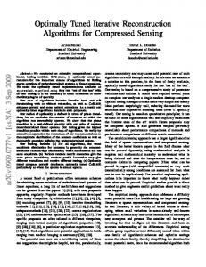
5.2. Phantom Experiments A. Simulated Cylindrical Phantom Studies A computer generated, hollow, uniform, cylindrical phantom was used to evaluate the correction of geometric response distortions. The inner radius of the cylinder was 5.1 cm and the outer radius was 6.4cm. The projection data were formed by a ray-driven, geometric response projector which models a fan beam collimator (hole diameter = 3 mm, length = 3.6 cm, focal length = 60 cm). The collimator traveled in an elliptical orbit, whose semiaxes were 36.5 cm and 6.5 cm, respectively. A 7x7 "inverse-cone" was implemented and 128 projections were obtained over 360".The projection array was 64x64 for each projection. Figures 12(a) and (b) show the projection data at 0" and 90°,respectively. The reconstruction of this cylindrical phantom without geometric response correction is shown in Figure 12(c), and witl! geometric response correction is shown in Figure 12(d). Both reconstructions were obtained after 50 iterations of the EM algorithm.
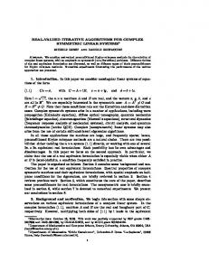
B. Jaszczak Phantom Studies Phantom studies were done using the Picker SX-300and
Parallel
Fan
Cone
I I I
atZl
0.1542 0.0640
0.1511
I I I I
at&
0.1790 0.2430 0.1113
I I I I
PRISM SPECT systems. The hot and cold rod circular Jaszczak phantom was used with 99mTc.A cone beam collimator (hole diameter = 1.89mm, length = 4 cm, focal length = 50 cm) study was performed on the SX-300and a parallel (hole diameter = 1.4 mm, length = 2.7 cm) and a fan beam collimator (hole diameter = 1.4 mm, length = 2.7 cm, focal length = 50 cm) studies were performed on the PRISM. For the cone beam study on the SX-300,128 projections were acquired at 300 seconds per projection. For studies on the PRISM, 120projections were acquired at 300 seconds per projection for the parallel hole collimator study and 240 seconds per projection for the fan beam collimator study. For each projection, the data were acquired into 64x64 arrays with 0.57cm bin width. The iterative EM reconstruction algorithm and ray-driven projector-backprojector were coded and results were obtained on an IBM 3090-600S supercomputer. The projections were matrix. Each reconstruction was reconstructed into a 64x64~64 obtained after 50 iterations of the EM algorithm. All projectorbackprojectors used a 7x7 "inverse-cone" to model the geometric response. The reconstructions of the Jaszczak phantom are shown in Figure 13.The results for the parallel (9.37~10~ total counts per slice), fan (2.86~10~ total counts per slice) and cone beam (5.54~10~ total counts per slice) collimators are given in the first., second, and bottom rows, respectively. The first column shows results after 50 iterations of the EM algorithm without geometric response and without attenuation correction. The second column shows results after 50 iterationswith attenuation correction but no geometric response correction. The third column shows results with geometric response correction but no attenuation correction. And the fourth column shows results. for geometric response correction and attenuation correction. The attenuation coefficient was assumed to be 0.15 cm-' within the phantom. A detailed description of the attenuation correction scheme is found in [17].
6. CONCLUSIONS In this paper, a three-dimensional iterative reconstruction algorithm which incorporates models of the geometric point response in the projector-backprojector is presented for parallel,
70 1
data in detector 1. In the EM algorithm, once a voxel value is set to zero, it will not change back to a non-zero value. Thus, in the subsequcnt iterations, the data from detector 2 cannot elongate the reconstructed point response. It is the zero background that “fixes” the distortion to zero. However, if the background is not zero, the iterative EM algorithm will reconstruct elongated point sourccs if the geometric response of the collimator is not propcrly modcled in the projector-backprojector.
ACKNOWLEDGMENTS The research work presented in this manuscript was partially supported by NIH Grant R01 HL 39792, the Whitaker Foundation, and Picker International. The authors thank Paul Christian for supplying the phantom data. A grant of computer time from the Utah Supercomputing Institute, which is funded by the State of Utah and the IBM Corporation, is gratefully acknowlcdgcd. We also thank Biodynamics Research Unit, Mayo Foundation for use of the Analyze software package.
REFERENCES Figure 12. Cylindrical phantom studies: (a) projection at O”, (b) projection at 90”, (c) reconstruction without geometric response correction, and (d) reconstruction with geometric correction. fan, and cone beam geometries. Reconstructed images are compared with and without modcling the geometric response and attenuation. Significant improvcments in image quality is shown when the geomctric point response and attenuation is appropriately compensatcd. It is observed that with attenuation correction alone resolution is significantly improvcd. The modeling of the geometric response is shown to accomplish a smoothing without loss of rcsolution. Our rcsults indicatc that the models are good approximations for the physics of the imaging system. A table for the geomctric point response is pre-calculatcd using closed form expressions. An “inverse-cone” structure is adopted in the ray-driven projector-backprojectors which use line length weighting. It is shown that the gcometric response is constant along each ray emanating from the projection bin. This result makes the algorithm more efficient. Attenuation factors are calculated in moving away from the dctcctor bin calculating the exponential of the linc integrals of the inuage attenuation distribution.
Finally, we make a brief comment concerning the reconstruction of an isolated point source using an iterative EM algorithm. A point sourcc reconstruction with an iterative EM algorithm can fool someone into concluding that an iterative EM algorithm which does not model gcomctric response gives equivalent results to one that does modcl gcometric responsc. Figure 14 illustrates a point source which is not at the center of rotation. A filler backprojection algorithm w i l l reconstruct an elongated point response, while an itcrativc EM algorithm will give a symmetric point response. Thc rcason for this is a unique property of the multiplicative E h l algorithm. In Figure 14, the data from detector 2 will attcmpt to broaden thc reconstructed result while the data from dctcctor 1 will make narrower thc elongated rcsult of detector 2 by zeroing thc rcsult to match the
I). E. Kuhl, R. Q. Edwards, “Reorganizing data from transverse section scans of the brain using digital processing,” Radiology, 1968, Vol. 91, p. 975-983. [ 2 ] J. F. Isenberg, W. Simon, “Radionuclide axial tomography by half back-projection,” Phys. Med. Biol., 1978, Vol. 23, p. 154-158. [3] I). J. Nowak, K. L. Eisner, W. A. Fajman, “Distance-weighted backprojection: a SPECT reconstruction technique,” Radiology, 1986, Vol. 159, p. 531-536. [4] E. Tanaka, “Quantitative image reconstruction with weighted backprojection for single photon emission computed tomography,” J. Comput. Assist. Tomogr., 1983, Vol. 7, p. 692-700. [ 5 ] M . A. King, K. R. Schwinger, R. C. Penney, “Variation of the count-dependent Meu filter with imaging system modulation transfer function,” Med. Phq’s., 1986, Vol. 13, p. 139-149. [6] R. M. W. Tsui and R. J. Jaszczak, “Incorporation of detector response in projector and backprojector for SPECT image reconstruction,” J . Nucl. Med., 1987, Vol. 28, p. 566. [7] R. R. Zeeberg, S. Loncario, H. N. Wagner and R. C. Reba, “A thcoretically-correct algorithm to compensate for a threedimensional spatially-varimt point spread function in SPECT imaging,”./. Nucl. Med. 1987, Vol. 28, p. 662P. [8] B. M. W. Tsui, G. T. Gullbcrg, H. B. Hu, J. G. Rallard, D. R. Gilland, J. R . Perry, W. H. McCartney, and T. Bemstein, “Applications of iterative reconstruction methods in SPECT.” In
[l]
7’hc Formation, Processing and Evaluation of Medical Imuges, NATO Advanced Sludy Institute, Povoa do Varzim, Portugal, September 12-23, 1988 (in press). 191 R. M. W. Tsui, H. R . Hu, I).K. Gilland, and G. T. Gullberg, “Implcmenta~ion of sirriul taneous attenuation and detector response correction in SI’ECT,” IEEE Trans. on Nucl. Sci., 1988, Vol. 35, pp. 778-783. [lOl A. K . Formiconi, A. Pupi, and A. Passeri, “Compensation of spatial system response in SPECT with conjugate gradient reconstruction technique,” Phys. Med. B i d , 1989, Vol. 34, NO. 1, pp. 69-84. 1111 K. Lang and K. Carson, “EM reconstruction algorithms for emission and transmission tomography,” J . Comput. Assist. Tomogr., 1984, Vol. 8, pp. 306-316. [12] E. C. Frey and R. M . W. Tsui, “Parameterization of scatter response function in SI’ECT imaging using Monte Carlo simulation,” IEEE Trans. on Nucl. Sci., 1990, Vol. NS-37, pp.
702
Figure 13. Jaszczak phantom reconstructions. (pl) Parallel, iterative EM; (p2) Parallel, iterative EM with attenuation compensation; @3) Parallel, iterative EM with geometric response correction; (p4) Parallel, iterative EM with geometric response corrections and attenuation compensation; (fl) Fan, iterative EM; (f2) Fan, iterative EM with attenuation compensation; (f3)Fan, iterative EM with geometric response correction; (f4) Fan, iterative EM with geometric response corrections and attenuation compensation;(cl) Cone, iterative EM; (c2) Cone, iterative EM with attenuation compensation; (c3) Cone, iterative EM with geometric response correction; (c4) Cone, iterative EM with geomctric response correction and attenuation compensation. 1308-1315. [13] S. Miracle, M. J. Yzuel, and S. Millan, “A study of the point spread function in scintillation camera collimators based on Fourier analysis,’’Phys. Med. Biol., 1979, Vol. 24, pp. 372-384. [14] C. E. Metz, F. B. Atkins and R. N.Beck, “The geometric transfer function component for scintillation camera collimators with straight parallel holes”, Phys. Med. B i d , 1980, Vol. 25, No. 6, pp. 1059-1070. [15] B. M. W. Tsui and G. T. Gullberg, “The geometric transfer function for cone and fan beam collimators,” Phys. Med. Bid., 1990,Vol. 35, No. 1, pp. 81-93. [16] G. T Gullberg, R. H. Huesman, J. A. Malko. N.J. Pelc, T. F. Budinger, “An attenuated projector-backprojector for iterative SPECT reconstruction,” Phy. Med. Bid., 1985. Vol. 30, pp. 799816. [17] G. T. Gullberg, G. L. Zeng, B. M. W. Tsui, and J. T. Hagius, “An iterative reconstruction algorithm for single photon emission computed tomography with cone beam geometry,” Int. J . Imug. Sys. & Techn.. 1989,Vol. 1,pp. 169-186.
Regular EM Reconstruction: Filter BackprojcctionReconstruction:
4 Dctector 1
0 Detector 2
... ............ .......................
Point Source
Figure 14. An example of point source study.