PROCEEDINGS, Thirty-First Workshop on Geothermal Reservoir Engineering Stanford University, Stanford, California, January 30-February 1, 2006 SGP-TR-179
THREE-DIMENSIONAL JOINT BAYESIAN INVERSION OF HYDROTHERMAL DATA USING AUTOMATIC DIFFERENTIATION V. Ratha, A. Wolfb, M. Bueckerb RWTH Aachen University Applied Geophysics, Lochnerstr 4-20, D-52056 Aachen, Germany e-mail:
[email protected] b Scientific Computing, Seffenter Weg, 23, D-52074 Aachen, Germany e-mail: [wolf,buecker]@sc.rwth-aachen.de a
ABSTRACT We have developed a Bayesian inverse modeling tool for the joint inversion of hydraulic and thermal data. It is based on a well-known and well-tested forward modeling code, which solves the coupled steady state equations for heat and mass transfer. Because of the heat and pressure dependence of most petrophysical properties, this is a nonlinear problem. Different nonlinearities of petrophysical properties and porespace models can be employed. The forward code was automatically differentiated to obtain partial derivative information. This information was used in several optimization schemes (Gauss-Newton, QuasiNewton, Nonlinear Conjugate Gradients) to find the minimum of the Bayesian objective function. In addition to the optimum model, the Bayesian approach supplies linear estimates of posterior covariances and related measures of uncertainty. We will present several instructive synthetic investigation demonstrating the power of the approach. Additionally, sensitivites and their use for the optimization of experimental design are discussed. INTRODUCTION Inverse models have turned out to be indispensable tools not only for model calibrations, but also for the evaluation of the uncertainty inherent to any inference from measured data. Inverse models, however, have much higher complexities when compared to the corresponding forward models, as the Jacobian J , i.e. the derivative of the forward model, g(p) , with respect to the parameters, p , is required. In addition, forward models are often well-tested codes, but nearly never designed with inverse applications in mind. It this situation, the method of Automatic Differentiation (AD, Bischof et al., 1996; Griewank, 2000) of-
fers an viable alternative to both, numerical differentiation and the often tedious formulation of continuous adjoints (Sun, 1994). In contrast to the calculation of derivatives by divided differences AD implies no additional truncation error. Details on this methods can be found on the internet portal .
BAYESIAN INVERSION The inverse toolbox described here is based on straightforward use of Bayesian theory (Tarantola, 2004). Here, the objective function Θ B = (d − g (p ))T Cd−1 (d − g (p )) + (p − p a )T C p−1 (p − p a ) (1)
is minimized, where several optimization algorithms can be used: Gauss-Newton (GN, requiring the full Jacobian) in parameter and data space, Nonlinear Conjugate Gradient (NLCG), and Quasi-Newton (QN) techniques are available (Nocedal & Wright, 1999). A Gauss –Newton formulation leads to the iterations in parameter and data space, p k +1 = p a + (J T C−d 1J + C−p1 )−1 ⋅ J T C−d 1[d − g (p k )] p k +1 = p a + C p J T (JC p J T + Cd ) −1 ⋅ [d − g (p k )]
(2)
Uncertainties for estimated parameters can be calculated from the corresponding covariance matrix a posteriori, −1 T −1 Capo p = ( J Cd J + C p )
−1
= C p − C p J T (JC p J T + Cd ) −1 JC p
(3)
Both forms have their merits depending on the number of data and parameters, or which kind of covariance information is available.
By now, data can be simple functions of nodal values of T or h calculated by forward model, or linear combinations, i. e., point measurements, gradients or integrals of both data types. Parameters to be inverted are porosity φ , hydraulic permeability k , thermal conductivity λ , and heat production A for each unit, and boundary conditions represented by low-order polynomials. Permeability k , as well as λ , are assumed to be anisotropic and have been parameterized by their vertical component and anisotropy factors. To guarantee positivity, and to improve scaling, parameters can be replaced by their natural logarithm. This amounts to a scaling of the Jacobian. Physical parameters are assigned to the grid cells by means of an index array. In order to keep the size of the inverse problem moderate, the parameters of interest may be assigned to geological units with homogeneous properties, which may represent for instance layers, isolated bodies, or fault zones. The current code gives the user considerable freedom to choose the appropriate setup for a given problem.
For the inversion outlined above, derivative information, be it the full Jacobian or the gradient. The forward problem described here is given by a FD discretization of the coupled nonlinear PDE for fluid flow and heat transport, ρf g k∇h + Q = 0 µf
(4)
and ∇ ⋅ λ e∇T − ( ρ c) f vT + A = 0 ,
Typically, AD is applied in “forward mode” or “reverse mode”. In the former case, code is generated capable to compute the derivative of many dependent variables with respect to a few independents (or linear combinations of the Jacobian columns) very efficiently. The nested function G(x) ∈ ℜM×ℜN discretized in the given program can be written as G (x) = G P (G P −1 (K G1 (G 0 ))) ,
(6)
with G 0 = x When only projections in the data or parameter space into given directions x% ∈ ℜM or N y% ∈ ℜ are used. These can be computed efficiently by x% T ⋅ g x = x% T ⋅ g10 (G 0 ) ⋅ g12 (G1 ) ⋅ K ⋅ g PP −−12 (G P − 2 ) ⋅ g PP −1 (G P −1 ) ,(7)
AUTOMATIC DIFFERENTIATION
∇⋅
differences involve truncation error. From a computer science point of view, automatic differentiation is similar to a compiler in that it transforms a given program into a new program. However, unlike a compiler, AD changes the semantics of a given program by inserting additional statements for the computation of derivatives.
(5)
where the λe marks effective thermal conductivity of the porous medium while µ f and ( ρ c) f the fluids dynamic viscosity and volumetric heat capacity. The nonlinear coupling is caused by temperature and pressure dependencies of the matrix and fluid properties, and thus the Darcy velocity v . We used the AD tool ADIFOR (Bischof et al., 1996) to generate derivatives of the modeling code. In AD, a program is conceptually decomposed into a finite sequence of elementary operations, e. g., addition, multiplication, and basic functions. From a mathematical point of view, this represents a composition of a potentially extremely large number of simple functions whose derivatives are known. So, the derivatives of the complete sequence are given by accumulating the derivatives of the known elementary functions according to the chain rule of differential calculus. Neglecting rounding errors, the values produced by this technique are exact, whereas values computed by numerical differentiation using divided
where the order of evaluation is from left to right (“forward mode”) and the the small g ik represent the derivatives of G i with respect to G k . In the second case, y% ⋅ gTx = y% ⋅ g PP −1 (G P −1 ) ⋅ g PP −−12 (G p − 2 ) ⋅ K ⋅ g12 (G1 ) ⋅ g10 (G 0 ) , (8)
represents the “reverse mode”, again evaluating from left to right. If we need to compute linear combinations of the rows efficiently, the “reverse mode” is the method of choice. In particular, the derivative of a scalar function as Eq. (1), i. e., its gradient, can be calculated at the price of a few forward solutions independent of the number of parameters (Griewank, 2000). This is important if we want to use the alternative optimization algorithms mentioned in above (NLCG, LBFGS) efficiently, as these only need the value of the objective function and its gradient. They are the methods of choice when dealing with large scale problems. by now, however, only the forward mode is operational.
h (m)
5950
surface boundary conditions
forced convection free convection
5900
unit # 11 10 9 8 7 6 5 4 3 2 1
11
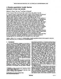
Fig. 1 Model geometry for synthetic models. It is constructed from 11 units of different thermal and hydraulic properties. For each unit, hydraulic permeability and thermal conductivity are given by true/prior/error, where error is defined as the square root of the variance a priori, based on the natural logarithm of the parameters. Units 1–8 represent sedimentary layers, while the salt diapir is associated with unit 9. The crosscutting faults which in this model are highly permeable, are units 10 and 11. Also shown is the assumed surface head driving the flow
SYNTHETIC MODEL To give an example, we calculated synthetic coupled 2-D models, schematically presenting the surroundings of salt diapir with cross-cutting tectonic faults. Model geometry (220 × 119) and the association of units is shown in Fig. 1. Unit 9 is associated with the nearly impermeable salt diapir, while units 10 and 11 represent the permeable fault zones. This geometry is the same in both models presented, differing mainly in the driving forces and the values of permeability associated with the main units. The model presented here is driven predominantly by a gradient of head imposed as a “topographic” boundary condition at the top (“forced convection”). Considerable flow occurs orthogonal to the temperature isolines, i. e., v ⋅ ∇T ≠ 0 in many areas of the model. Temperatures and heads for this model as well as some sensitivities calculated by AD are shown in Fig. 2. The sensitivities display complicated, and sometimes contra-intuitive interrelations. The sensitivities shown here differ considerably from the ones calculated for flows driven by density differences, i. e., “free convection” . Thus the choice of data necessary for a successful inverse model depends strongly on the assumed model, e. g., boundary conditions. Though their values can in principle be obtained by the inversion, a conceptual model must be available in advance. Sensitivities of the different data types sometimes complement each other, thus motivating hope
that the joint inversion may produce better results than the ones based on head or temperature alone.
NUMERICAL EXPERIMENTS For the numerical experiments in the following we used the model setup described in Fig. 1. For each case, a set of 8 models was created. In each of these models, a given number of boreholes were generated, choosing site and depth at random. In particular, depth varied normally with a mean of 3500 m and a standard deviation of 1000 m. The data were subsequently modified, adding zero-mean normal noise with a standard deviation of 0.5 K for temperature, and 0.5 m for head, respectively. This choice of errors is of course disputable: though temperature can be continuously measured at high accuracy, technical and geological noise may easily reach this value. By geological noise we refer to small-scale parameter variations not accounted for in the model. The quasicontinuous head observations are somewhat ideal zed, because formation pressure is difficult to obtain in deep boreholes as assumed here. Often only integral values for special intervals or other derived quantities (e. g., Darcy velocities) are known. These conditions could be considerably different in a shallower regime, where temperature differences may be much smaller, and heads are much easier to determine with high accuracy. A typical fit for this type of model is shown in Fig. 3. (a)
(b)
(c)
(d)
(e)
(f)
Fig. 2 Sensitivities of temperature (left) and hydraulic head (right) with respect to the natural logarithm of isotropic permeability for zones 11 and 7 marked in Fig. 1. Top: Temperatures and hydraulic heads for this model. Also shown are the Darcy velocities. Center: permeability derivative unit 11 (high-permeability fault zone). Bottom: same for unit 7.
0
Temperature
variances if more boreholes are includes. For this complex synthetic case, the necessary number of boreholes is rather high. -12
Forced Convection
(a)
Permeability
-14
-16 log10 k (m-2 )
For each of these models inversions were run to 50 iterations. For some of the more problematic models, this turned out to be too few, but for nearly all of these, convergence could be obtained after 100 iterations. Note that the parameters were taken as natural logarithms, implying that permeability errors of 6 correspond to a factor of more than two decades, while conductivities are usually believed to be more accurately known ( ≈ 20%). The priors were chosen with a non-trivial setup in mind, not making the inversion too easy.
1000
-18
-20 obs calc
true
2000
prior
z (m)
-22
prior variance 3000
-24
4000
1
2
3
4
5
6
7
8
9
10
11
1
(b) 5000
0
50
100
150
0.5
T
h+T h
-1
-1
log10 λ (W m K )
Temperature (°C)
obs calc
0 true prior
Thermal Conductivity
prior variance
Hydraulic Head
-0.5 5900
5910
5920
5930
5940
5950
Hydraulic Head (m)
Fig. 3 Typical data fit for hydraulic potential (head) and temperature. The numerical experiment presented in Fig. 4 demonstrates the role of different data types. Temperature, head, and joined data sets were generated as described above. As expected, the determination of thermal conductivities requires temperature measurements. However, in cases with significant flow, the use of hydraulic data will reduce uncertainties, as advective effects may inhibit the direct estimate of thermal properties. The numerical experiment presented in Fig. 5 aimed at demonstrating how strongly the results depend on number and choice of the boreholes. For this purpose, we generated subsets of 8 models with different numbers of random boreholes used, choosing 4, 8, and 12 for this number. Again, inverse solutions were obtained for all of these. For 4/8/12 boreholes, 2/1/1 inverse runs did not reach a value of the objective function which was considered small enough during the first 50 iterations and thus were not included. As expected, estimates show lower
1
2
3
4
5
6 7 unit #
8
9
10
11
Fig. 4 Inversion results for temperature data (blue upward triangles, shifted to the left), head data (red downward triangles, shifted to the right), and the combined data set (green circles, center). Error bars were calculated from Eq. (3).
MODELL-BASED EXPERIMENTAL DESIGN Curtis (2004a,b) gives an excellent introduction on the methods of experimental design. The simplest indicators of design quality are based on the Fisher information matrix, F = J T J , which is easily available from the inverse solution. If the SVD of J is calculated, and λi are the singular values, some common choices are N
1 i =1 λi + δ
D0 = −∑ N
D1 = ∑ λi = trace(F) , i =1 N
D2 = ∏ λi = det(F) i =1
where δ is an appropriately chosen threshold.
(9)
-12
Forced Convection
(a)
Permeability
-13
log10 k (m-2 )
require the optimization with respect to multiple objectives.
-14
CONCLUSIONS
-15
We have shown that AD is a valuable tool for the development of inverse codes from complicated existing forward models. Though the approach described is not fully automatic, it offers great advantages. The technique does not introduce additional truncation error. It is particularly easy to integrate changes in the underlying physics or new discretization schemes. From the sensitivities thus derived, we can conclude that by a model-derived placement of boreholes or measurements the amount of data necessary to estimate properties of a given structure to an given accuracy may be considerably reduced. The availability of the full sensitivity matrix thus may give the possibility to employ formal methods of experimental design for this purpose. The optimization tasks associated with this problem remain an important and challenging task for the future. Ongoing and future developments include: (1) field studies in a regional basin regime (2) the generalization to time-dependent problems; (3) the use of more advanced parameterizations; (4) the application of AD in ”reverse” mode to take advantage of better optimizers;(6) the integration of new physics and data types, e. g., salinities, or electrokinetic potentials (Titov et al., 2005; Yasukawa et al., 2003).
-16 -17 -18 -19 true
-20
prior -21
prior variance
-22
1
2
3
4
5
6
7
8
9
10
11
1
log10 λ (W m-1 K-1 )
(b)
0.5
4
8
12
0 true prior
Thermal Conductivity -0.5
1
2
3
4
5
6 unit #
prior variance 7
8
9
10
11
Fig. 5 Inversion results for data sets combined from 4 (red upward triangles, shifted to the left), 8(green circles, center), and 12 (blue downward triangle, shifted to the right) boreholes, chosen at random in the way described in the text. As it had to be expected, variances show an inverse relation to the number of boreholes. ‘Focused’ versions of these indicators may be calculated from a modified Jacobian, constructed from a subset of parameters, or by more advanced the techniques. Other indicators, e.g. based on the covariance matrix a posteriori are possible. Curtis (1999) has shown that though basing on the distribution of singular values, the different criteria may emphasize different features. Thius for any optimization they have to be carefully chosen and/or combined. In practice these “simplistic” design criteria will be of little use. Combined with appropriate constraints and weightings, however, they may produce valuable results in an iterative process of experimental design and model update. Optimizing an experimental layout, and in later stages production will require advanced optimization methods, as these functions display many extrema, and any particular design may
REFERENCES Aster R., Borchers B., Thurber, C. (2004), “Parameter estimation and inverse problems”, Academic Press, San Diego. Bischof, C., Carle, A., Khademi, P., and Mauer, A. (1996), “ADIFOR 2.0: Automatic differentiation of Fortran 77 programs”, IEEE Computational Science & Engineering, 3, 18-32. Curtis A. (2004a), “Theory of model-based geophysical survey and experimental design. Part Alinear problems”, The Leading Edge, 23, 997-1004. Curtis A. (2004b), “Theory of model-based geophysical survey and experimental design. Part Bnonlinear problems”, The Leading Edge, 23, 11121117. Griewank A. (2000), “Evaluating Derivatives. Principles and techniques of algorithmic differentiation”, SIAM, Philadelphia. Nocedal, J., Wright, S. J. (1999), “Numerical Optimization”, Springer, New York. Sun, N.-Z. (1994), “Inverse problems in groundwater modeling”, Kluwer, Dordrecht. Tarantola, A. (2004). “Inverse Problem Theory. Methods for model parameter estimation”, SIAM, Philadelphia. Titov K., Revil A., Konosavsky P., Straface S., Troisi S. (2005) ”Numerical modelling of self-
potential signals associated with a pumping test experiment”, Geophys. J. Int., 162, 641–650. Yasukawa, K., Widarto D., Mogi T., Ehara S. (2003), “Numerical modeling of a hydrothermal system around Waita volcano, Kyushu, Japan, based on resistivity and self-potential survey results”, Geothermics, 32, 21–46.