Available online at www.sciencedirect.com Available online at www.sciencedirect.com
Procedia Engineering
Procedia Engineering 00 (2011) 23 000–000 Procedia Engineering (2011) 53 – 59 www.elsevier.com/locate/procedia
PEEA 2011
Three-dimensional surface modeling using intelligent database techniques Somia M. El_Hefnawy Engineering Mathematics and Physics Dept., Faculty of Engineering, Mansoura University, Mansoura, EGYPT. e-mail:
[email protected]
Abstract Range image acquisition can be defined as the process of determining the physical distance from a given observation point to all points of consideration in a three-dimensional (3D) surface object. The technology of range finders has been used for many years in military and airborne remote sensing survey applications. This paper suggests the use of computer databases (instead of mathematical formulas) for modeling 3D surfaces. The basic concept is the proper selection of representative samples from the measured range values to be records in the model database. The main contribution in this paper is developing an Intelligent Database Management System (IDMS) used for selecting samples and giving depth prediction at a given space point. The IDMS performs standard database operations such as adding, updating and deleting records in order to minimize the data storage memory size and prediction error. Search for specific data which are not previously stored in the database is impossible in classical database management systems (DMS).
© 2011 Published by Elsevier Ltd. Open access under CC BY-NC-ND license. Selection and/or peer-review under responsibility of [PEEA 2011] Keywords:- 3D Imaging; Surface Modeling; Range Finder Applications; Database Management Systems; Computational Physics.
1. Introduction The goal of surface reconstruction is to obtain a continuous representation of a surface described by a given cloud of points. This problem is often called the unorganized points problem because the cloud of points has no connectivity information [1]. The motivation behind surface reconstruction is to obtain a digital representation of a real world, physical object or phenomenon [2,3]. Clouds of point data may be obtained from medical scanners (X-rays, MRI), range finders (optical, sonar, radar), or vision techniques (correlated viewpoints, voxel carving, stereo range images). Often, additional information on the cloud of points may be available, such as the order in which the data points were sampled, the orientation of the
1877-7058 © 2011 Published by Elsevier Ltd. Open access under CC BY-NC-ND license. doi:10.1016/j.proeng.2011.11.2464
254
Somianame M. El_Hefnawy / Procedia Engineering 23 (2011) 53 – 59 Author / Procedia Engineering 00 (2011) 000–000
normal vector at each of the points, or the positions of the cameras used in stereo range images [4,5]. The main concern of this paper is to develop a technique for selecting the surface representative points in order to minimize the used memory size and surface reconstruction error. The computer database concept is employed for solving this problem. In fact, if some strong a priori knowledge on the object is available such as parametric descriptions, then a single view allows shape recovery [6,7], object pose estimation and object recognition [8,9,10]. For any smooth object, a sequence of occluding contours must be considered to recover the shape [11,12,13]. 2. Surface modeling problem using measurement data Given:- i)A set of surface points provided by the range finder system represented as Srf = {(xi, yi, zi)| 1 ≤ i ≤ N}, where N is the number of the scanned points. The values (xi, yi) represent planar coordinates of ith measurement and zi is the corresponding depth value provided by the range finder. ii) An array M with dimensions [L x 3] stores numerical real values and L < N. A single row in this array is used to store the three coordinates (xp, yp, zp) of a surface point selected from the set Srf. Required:- i) Select L members of Srf to construct the set Smodel= {(xi, yi, zi)| 1 ≤ i ≤ L}. Smodel must represent the scanned surface. The members of Smodel are stored in the array M. m
ii) Develop an algorithm to estimate a depth value z g for given coordinates (xg , yg) using the model Smodel. The position (xg , yg) of a given surface point may or may not be the planar coordinates of a member in the original set Srf. m
Constraints:- i) The subset Smodel must be chosen such that the prediction error eg = |zg – z g | for any given point (xg , yg, zg) in the original set Srf is within a specific range εerror defined by the model designer, i.e., eg < εerror. ii)The selected set Smodel must have a length L as small as possible to optimize the used computer memory. From the computer point of view, the set Smodel represents a database. The array M is the single table in this database. The table M can be written as M = [ R1 R2 R3 …… RL]T. The ith record Ri = [xi yi zi]T is the ith member in Smodel. The three coordinates xi , yi , zi are the different fields of the corresponding record. If qx, qy, qz are the numbers of bytes used to store xi , yi , zi respectively (according to the chosen data types), then the total memory size required to store this database is (qx + qy + qz)L [bytes]. 3. Database model for 3D surfaces A new solution is proposed for solving the reconstruction problem in which no unique set of mathematical equations are used to represent the surface. The solution space defines the set of all candidate solutions that may be evaluated as possible solutions to the problem. For N samples the number of combinations to choose L samples (without repeating their elements in any order) is given as; ( LN ) = L!( NN−! L)! . The number of rows L in the array M[Lx3] is not known previously. Only the N constraint (1 < L < N) must be satisfied. Hence, only one combination N ! is decided (according to its . Generally, the number modeling accuracy), we have the total number of combinations − L)! For this reason, the L =1 L! ( Nproblem. of candidate solutions that can be evaluated is huge for non-trivial evaluation of the entire space of all candidate solutions is, however, usually completely impractical.
∑
355
Somia M. El_Hefnawy / Procedia Engineering 23 (2011) 53 – 59 Author name / Procedia Engineering 00 (2011) 000–000
3.1 Concept of neighborhood between space points Assume that the point P(x,y,z) in Srf is chosen randomly. Assume that the three points P1(x1,y1,z1), P2(x2,y2,z2), P3(x3,y3,z3) are the nearest surrounding neighbors to P(x,y,z) in the set Srf and lying on a planar surface s1, Fig. (1). From the principles of analytic geometry, the general equation for s1 is: x y z 1 x1 y1 z1 1 (1) =0 x2 y 2 z 2 1 x3 y3 z3 1 This equation can be written as:
z = w1 z1 + w2 z 2 + w3 z3
w1 = [( x3 − x2 ) y + ( x − x3 ) y2 + ( x2 − x ) y3 ] / D w2 = [( x3 − x ) y1 + ( x1 − x3 ) y + ( x − x1 ) y3 ] / D
where;
w3 = [( x − x2 ) y1 + (x1 − x ) y 2 + ( x2 − x1 ) y ] / D
(2) (3a) (3b) (3c)
D = ( x3 − x2 ) y1 + (x1 − x3 ) y 2 + ( x2 − x1 ) y3 (4) ( ) The condition D ≠ 0 must be satisfied to guarantee that the three points P1, P2, P3 lie on the same
And
plane. Assume that the three points P1(x1,y1,z1), P2(x2,y2,z2), P3(x3,y3,z3) are selected as a model representing the investigated surface which is approximated by s1 in their neighborhood. According to eq. (2) the depth z at point P is predicted from depth values at the selected three neighbors z1, z2, z3 weighted by w1, w2, w3 respectively. According to eqs. (3-3), these weights vary from a planar position (x,y) (at which the depth z is required) to another according to the planar positions of the selected neighbors in the surface model. Also, eq. (2) suggests a local prediction formula to test whether a measured depth provided by a range finder at certain planar position belongs to s1 plane or not. There are two basic conditions to be satisfied for the three points P1, P2, P3 used to represent the planar patch containing the randomly selected point Pi in Srf. The first is that, P1, P2, P3 are as near as possible to Pi and the second is that, P1, P2, P3 surround Pi. The nearest neighborhood condition can be measured as the summation di123 of the Euclidian distances di1, di2, di3 between Pi and P1, P2, P3 respectively, i.e., d i123 = d i1 + d i 2 + d i 3 (5) And
d in = ( xi − xn ) 2 + ( yi − yn ) 2 + ( zi − z n ) 2 , n=1,2,3
(6)
To develop a condition for testing that Pi is surrounded by P1, P2, P3, we will consider the areas of the triangles formed in the plane OXY by the projections of these points denoted as vi, v1, v2, v3. The triangle formed by vertices v1, v2, v3, has the area A123 determined by the formula: A123 = 0.5v23 h123 (7) where v23 is the side length between the two vertices v2,v3 and h123 is the perpendicular height from vertex v1 on the side v23. After few mathematical manipulations the following formula can be derived: 2 2 2 2 2 0 .5 (8) A123 = {[( x1 − x2 ) + ( y1 − y 2 ) ][( x3 − x 2 ) + ( y3 − y 2 ) ]− [( x1 − x 2 )( x3 − x 2 ) + ( y1 − y 2 )( y3 − y 2 )] } / 2 The pint Pi is surrounded by P1, P2, P3 if vi lies inside or on one of the sides of the triangle v1v2v3. Considering the case shown in Fig. (2-a), the following mathematical equation is satisfied; A123 = Ai12 + Ai13 + Ai 23 (9) where A123, Ai12, Ai13, Ai23 are the triangular areas formed in the plan OXY by the vertices v1, v2, v3 , vi . If Pi is not surrounded by P1, P2, P3 as shown in Fig. (2-b) where vi faces a single side of the triangle v1v2v3 then we have:
456
Somianame M. El_Hefnawy / Procedia Engineering 23 (2011) 53 – 59 Author / Procedia Engineering 00 (2011) 000–000
A123 = Ai12 + Ai13 − Ai 23
(10)
Considering the case shown in Fig. (2-c) in which vi faces two sides of the triangle v1v2v3 from outside, the following equation is satisfied: A123 = Ai12 − Ai13 − Ai 23 (11) 3.2 Concept of information content Assume that the point Pi(xi,yi,zi) is selected randomly from Srf during the model building process. Assume also that the surface model contains the three points P1, P2, P3 chosen near to and around P1 according to the conditions explained in the previous section. The criteria used to add the point Pi to the m surface model need to be investigated. Substituting the values (xi,yi) into eq. (2), the value zi can be m determined. The value zi is considered as the predicted depth at position (xi,yi) provided by the recent surface model having P1, P2, P3 as members. If ε error is the acceptable level of accuracy for the surface approximation, then according to the absolute difference zi − zim , the following two cases can be considered:• z i − z im ≤ ε error . In this case, the investigated point Pi(xi,yi,zi) in the given set Srf does not contribute
•
to the information content represented by the recent model. In this case, there is no need to add the point Pi(xi,yi,zi) to the recent model. The surface can be reconstructed by the 3D triangle patch P1P2P3 in the small neighborhood around Pi(xi,yi,zi). z i − z im > ε error . In this case, the point Pi(xi,yi,zi) is a key point and must be added to the model
library because it can not be predicted correctly by the recent model. After adding the point Pi(xi,yi,zi) to the model, the surface can be constructed by using the shape consisting of the three triangles patches PiP1P2, PiP1P3, PiP2P3. Assume that the point Pi selected randomly from Srf during the model building process does not have P1, P2, P3 surrounding it (this occurs if vi lies on the border of the projections of Srf points on the OXY plane). The criteria used to add the point Pi to the surface model can be developed using only the first nearest three points (constituting a planar triangle) to Pi. Substituting the values (xi,yi) into eq. (3-2), the m value zi can be determined. As in the previous case, if the absolute difference z i − z im ≤ ε error , there is no need to add the point Pi(xi,yi,zi) to the recent model and the surface can be reconstructed by extending the 3D triangle patch P1P2P3 in the small neighborhood around Pi(xi,yi,zi). If the estimation accuracy is not accepted, then the point Pi(xi,yi,zi) must be added to the model. In this case we have two possibilities for constructing the 3D surface in the investigated neighborhood. • The vertex vi faces a single side of the triangle v1v2v3 where eq. (10) is satisfied. The 3D surface in the investigated neighborhood can be constructed by two triangular patches. The first patch is P1P2P3 and the second is PiP2P3. The two patches have the common side P2P3. • The point vi faces two sides of the triangle v1v2v3 where eq. (8) is satisfied. The 3D surface in the investigated neighborhood can be constructed by three triangular patches. The three patches are P1P2P3 , PiP1P2 , PiP2P3. These patches have the common sides P2P3 , P2P3 , P2P3. For a given point Pi, the selected three points P1, P2, P3 in the surface model satisfying the two conditions of neighborhood explained previously will be denoted as model prediction points. 3.3 Database management system for the surface model The algorithm receives the elements in Srf and investigates its information content. Building the surface model is an iterative process. It starts by selecting randomly a single point Pi of the given Srf and applying
557
Somia M. El_Hefnawy / Procedia Engineering 23 (2011) 53 – 59 Author name / Procedia Engineering 00 (2011) 000–000
the previously described processes for finding the nearest surrounding three points in Srf. The initial surface model Smodel consists of these three points and may or may not include the point Pi according to the prediction accuracy of its depth value using the chosen three points. These points represent the initial records in the model database. The model building process continues by selecting another random point Pi from Srf. A systematic way for investigating all the groups consisting of three points in Smodel is used to find the model prediction points for this new point Pi. The database model is updated by adding the randomly selected point to the model if the prediction accuracy of its depth value is not good, else the model is not updated 4.Computer simulation experiments In the first simulation a spherical surface z = 49 − ( x + y ) with radius equals 7 units and center at origin is investigated. The domain used is D = ( x, y ) − 10 ≤ x ≤ 10, − 10 ≤ y ≤ 10 . Only the upper half of the sphere is scanned with the viewing direction along OZ-axis. The number of samples used is 1000 points chosen randomly in the specified domain. The approximation error was set to be 5% of the sphere radius. Two runs of the program were performed. In the first run, the model database is updated by adding a new record after processing every sample when the error in depth prediction exceeds the allowed limits but the information content analysis of the database records is not performed. This case is denoted as non-optimized surface model. In the second run of the program, the information content analysis is performed for the whole database records after adding a new record to the model database. This case is denoted as optimized surface modelIt is evident form part (a) in Figs. (3,4) that, as the samples are feeded to the system, the prediction error decreases especially after the first one hundred samples. Comparing the models in Figs. (3b, 4b), it is evident that the size of the optimized database model is 94 records while the nonoptimized one has a size equals 241 records. This means that, the optimized database size is 39% of the size of the nonoptimized one. Comparing the error patterns in the two cases, it seems that the variance of the prediction error after the first one hundred samples for the optimized database is little bit more than the nonoptimized one, but the difference in the average error values between the two cases can be neglected. In the second simulation a more difficult function surface, referred to as the pulse function is used. It is represented as the shape of the surface corresponding to the 2 2 radially symmetrical bivariate function z = 10 Sin(r ) / r , where r = x + y is the distance along the OXY plane to the origin (0,0). The domain used is D = ( x, y ) − 10 ≤ x ≤ 10, − 10 ≤ y ≤ 10 . We want a “sharper peak”, so we will scale the x and y variables with a factor 2π. The approximation error was set to be 5% of the maximum peak value. The results similar to the previous simulation are obtained in Figs. (5,6). Comparing the models in Figs. (5b, 6b), it is evident that the size of the optimized database model is 90 records while the nonoptimized one has a size equals 264 records. This means that, the optimized database size is 34.1% of the size of the nonoptimized one. The error variation with the sample time index gives a similar indication as in the case of the spherical surface.
{
2
2
{
Fig. (1) Approximating a surface by a triangular patch around a point
}
}
Figure (2) Relationships between projection areas
658
(a) Error variation with sample index
Somia M. El_Hefnawy / Procedia Engineering 23 (2011) 53 – 59 Author name / Procedia Engineering 00 (2011) 000–000
(b) surface model
(a) Error variation with sample index
(b) surface model
Fig. (3) Spherical surface results (non-optimized )
Fig. (4) Spherical surface results (optimized model)
(a) Error variation with sample index
(a) Error variation with time
(b) surface model
Fig. (5) Pulse surface results (non-optimized model)
(a) Error variation with sample index
(b) surface model
Fig. (6) Pulse surface results (optimized model)
(b) surface model
Fig. (7) Cubic surface results (non-optimized model)
Investigating the optimized models for both spherical and pulse surfaces (Figs. 4b, 6b respectively) to notice the distribution of the model points, it can be found that a lot of samples are concentrated near the perimeter of the circle representing the projection of the scanned upper half of the sphere, while less samples are concentrated near the top of the sphere as viewed across OZ axis. For the pulse surface a lot of samples are concentrated near the center of the pulse peak projection compared to the perimeter area. A third simulation is performed. A discontinuous function that looks like a cube with the side-walls and bottom removed Fig. (7) shows the results for a non optimized model case. It is evident that among of 274 model points only 4 to 7 points exist on the planar top of the box. The remainder of the points (about 270 point) exist near the discontinuity regions in the four sides of the box. This proves the result that discontinuities needs more points to catch its representation. 5. Conclusion This paper presents a technique for developing a surface model of 3D physical object acquired as clouds of 3D points. Computer database model is constructed using selected surface points. The depth is estimated using a simplified prediction routine The proposed method begins with a rough approximation of the surface using less number of points and progressively refines it in successive steps in the regions where the data are poorly approximated. The adaptive method for adding, deleting and updating database records is simple in concept, yet realizes efficient data reduction. Furthermore, as it refines locally the triangular surface without reconstructing the entire surface, the method is efficient in computational time. Computer simulation results are given to show that the surface models are compact and faithful to the
Somia M. El_Hefnawy / Procedia Engineering 23 (2011) 53 – 59 Author name / Procedia Engineering 00 (2011) 000–000
original data points. It was found that generally, the system needs more points in the regions which have sharp variation in the surface gradient compared to the regions with less gradient variations References [1] J.H. Rieger, Optics Letters, 11: 123-125, 1986. [2] M.P. do Carmo, Prentice-Hall, Englewood Cliffs, New Jersey, 1976. [3] O. Faugeras, Artificial Intelligence. MIT Press, Cambridge, 1993. [4] J. Porrill and S. Pollard, Image and Vision Computing, 9(1): 45-50, 1991. [5] W.B. Seales and O.D. Faugeras, Computer Vision and Image Understanding, 61(3): 308-324, 1995. [6] J. Ponce, D. Chelberg, and W.B. Mann, IEEE Transactions on PAMI, 11(9): 951-966, 1989. [7] M. Zerroug and R. Nevatia, Proc. of IEEE Conf. on Comp. Vision and Pattern Recognition, New York (USA), pp: 96-103, 1993. [8] D. Kriegman and J. Ponce, IEEE Transactions on PAMI, 12(12): 1127-1137, December 1990. [9] R. Glachet, Thèse de doctorat, Université Blaise Pascal de Clermont-Ferrand, 1992. [10] D.A. Forsyth, and J.L. Mundy, Proc. of 2nd Euro. Conf. on Comp. Vision, (Italy), pp. 639-647, May 1992, V. 588. [11] M.-O. Berger, Proc. of the 12th Int. Conf. on Pattern Recognition, Jerusalem (Israel), volume 1, pages 32-36, 1994. [12] R. Cipolla, K.E. ström, and P.J. Giblin, Proc. of 5th Int. Conf. on Computer Vision, Boston (USA), pages 269-275, June 1995. [13] H. Fuchs, Z.M. Kedem, and S.P. Uselton, Communications of the ACM, 20(10): 693-702, 1977.
7 59