The Dynamic Time Warping (DTW) distance measure is a technique that has long been known in speech recognition community. It allows a non-linear mapping ...
Three Myths about Dynamic Time Warping Data Mining Chotirat Ann Ratanamahatana
Eamonn Keogh
Department of Computer Science and Engineering University of California, Riverside Riverside, CA 92521 { ratana, eamonn }@cs.ucr.edu Abstract The Dynamic Time Warping (DTW) distance measure is a technique that has long been known in speech recognition community. It allows a non-linear mapping of one signal to another by minimizing the distance between the two. A decade ago, DTW was introduced into Data Mining community as a utility for various tasks for time series problems including classification, clustering, and anomaly detection. The technique has flourished, particularly in the last three years, and has been applied to a variety of problems in various disciplines. In spite of DTW’s great success, there are still several persistent “myths” about it. These myths have caused confusion and led to much wasted research effort. In this work, we will dispel these myths with the most comprehensive set of time series experiments ever conducted.
Keywords Dynamic Time Warping, Data Mining, Experimentation.
1
Introduction
In recent years, classification, clustering, and indexing of time series data have become a topic of great interest within the database/data mining community. The Euclidean distance metric has been widely used [9], in spite of its known weakness of sensitivity to distortion in time axis [6]. A decade ago, the Dynamic Time Warping (DTW) distance measure was introduced to the data mining community as a solution to this particular weakness of Euclidean distance metric [2]. This method’s flexibility allows two time series that are similar but locally out of phase to align in a nonlinear manner. In spite of its O(n2) time complexity, DTW is the best solution known for time series problems in a variety of domains, including bioinformatics [1], medicine [4], engineering, entertainment [22], etc. The steady flow of research papers on data mining with DTW became a torrent after it was shown that a simple lower bound allowed DTW to be indexed with no false dismissals [6]. The lower bound requires that the two sequences being compared are of the same length, and that
the amount of warping is constrained. This work allowed practical applications of DTW, including real-time queryby-humming systems [22], indexing of historical handwriting archives [17], and indexing of motion capture data [5]. In spite of the great success of DTW in a variety of domains, there still are several persistent myths about it. These myths have caused great confusion in the literature, and led to the publication of papers that solve apparent problems that do not actually exist. The three major myths are: Myth 1: The ability of DTW to handle sequences of different lengths is a great advantage, and therefore the simple lower bound that requires different-length sequences to be reinterpolated to equal length is of limited utility [10][19][21]. In fact, as we will show, there is no evidence in the literature to suggest this, and extensive empirical evidence presented here suggests that comparing sequences of different lengths and reinterpolating them to equal length produce no statistically significant difference in accuracy or precision/recall. Myth 2: Constraining the warping paths is a necessary evil that we inherited from the speech processing community to make DTW tractable, and that we should find ways to speed up DTW with no (or larger) constraints[19]. In fact, the opposite is true. As we will show, the 10% constraint on warping inherited blindly from the speech processing community is actually too large for real world data mining. Myth 3: There is a need (and room) for improvements in the speed of DTW for data mining applications. In fact, as we will show here, if we use a simple lower bounding technique, DTW is essentially O(n) for data mining applications. At least for CPU time, we are almost certainly at the asymptotic limit for speeding up DTW. In this paper, we dispel these DTW myths above by empirically demonstrate our findings with a comprehensive set of experiments. This work is part of an effort to redress these mistakes. In terms of number of objective datasets and size of datasets, our experiments are orders of magnitude greater than anything else in the literature. In
particular, our experiments required more than 8 billion DTW comparisons. The rest of the paper is organized as follows. The next three sections consider each of the three myths above with a comprehensive set of experiments, testing on a wide range of both real and synthetic datasets. Section 5 gives conclusions and directions for future work. Due to space limitations, we decided to omit the datasets details and background/review of DTW (which can be found in [16]). However, their full details and actual datasets have been publicly available for free download at [8].
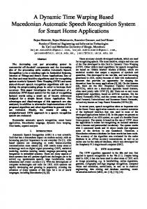
The variable-length datasets are then linearly reinterpolated to have the same length of the longest time series within each dataset. Then, we simply compute the classification accuracies using DTW for all warping window sizes (1% to 100%) for each dataset. The results are shown in Figure 1. 100
96.5
96
95
95.5 90
Face
85 94.5 80
94
93.5 0
20
40
60
80
100
75 0
20
40
60
80
100
99.5 100 99
99.9 99.8
98.5
99.7
2
Leaf
95
Does Comparing Sequences of Different Lengths Help or Hurt?
Trace
99.6
Wordspotting
98
99.5
97.5
99.4 97
99.3 99.2
96.5
99.1
Many recent papers suggest that the ability of classic DTW to deal directly with sequences of different length is a great advantage; some paper titles even contain the phrase “…of different lengths” [3][13] showing their great concerns in solving this issue. These claims are surprising in that they are not supported by any empirical results in the papers in question. Furthermore, an extensive literature search through more than 500 papers dating back to the 1960’s failed to produce any theoretical or empirical results to suggest that simply making the sequences to be of the same length has any detrimental effect. To test our claimed hypothesis that there is no significant difference in accuracies between using variable-length time series and equal-length time series in DTW calculation, we carry out an experiment as follows. For all variable-length time series datasets (Face, Leaf, Trace, and Wordspotting – See [8] for dataset details), we compute 1-nearest-neightbor classification accuracies (leaving-one-out) using DTW for all warping window sizes (1% to 100%) in two different ways:- (1) The 4S way; we simply reinterpolated the sequences to have the same length, and (2) By comparing the sequences directly using their original lengths. To give the benefit of the doubt to different-length case, for each individual warping window size, we do all four possible normalizations above, and the best performing of the four options is recorded as the accuracy for the variable-length DTW calculation. For completeness, we test over every possible warping constraint size. Note that we start the warping window size of 1% instead of 0% since 0% size is Euclidean distance metric, which is undefined when the time series are not of the same length. Also, when measuring the DTW distance between two time series of different lengths, the percentage of warping window applied is based on the length of the longer time series to ensure that we allow adequate amount of warping for each pair and deliver a fair comparison.
99 0
20
40
60
80
100
96 0
20
40
60
80
100
Figure 1. A comparison of the classification accuracies between variable-length (dotted lines) and the (reinterpolated) equal-length datasets (solid lines) for each warping window size (1-100%). The two options produce such similar results that in many places the lines overlap.
Note that the experiments do strongly suggest that changing the amount of warping allowed does affect the accuracy (an issue that will be discussed in depth in the next section), but over the entire range on possible warping widths, the two approaches are nearly indistinguishable. Furthermore, a two-tailed test using a significance level of 0.05 between each variable-length and equal-length pair indicates that there is no statistically significant difference between the accuracy of the two sets of experiments. An even more telling result is the following. In spite of extensive experience with DTW and an extensive effort, we were unable to create an artificial problem where reinterpolating made a significant difference in accuracy. To further reinforce our claim, we also reinterpolate the datasets to have the equal length of the shortest and averaged length of all time series within the dataset. We still achieve similar findings. These results strongly suggest that work allowing DTW to support similarity search that does require reinterpolation, is simply solving a problem that does not exist. The oftenquoted utility of DTW, such as “(DTW is useful) to measure similarity between sequences of different lengths” [21], for being able to support the comparison of sequences of different lengths is simply a myth.
3
Are Narrow Constraints Bad?
Apart from (slightly) speeding up the computation, warping window constraints were originally applied mainly to prevent pathological warping (where a relatively small section of one sequence maps to a much larger section of another). The vast majority of the data mining researchers have used a Sakoe-Chiba Band with a 10% width for the
global constraint [1][14][18]. This setting seems to be the result of historical inertia, inherited from the speech processing community, rather than some remarkable property of this particular constraint. Some researchers believe that having wider warping window contributes to improvement in accuracy [22]. Or without realizing the great effect of the warping window size on accuracies, some applied DTW with no warping window constraints [12], or did not report the window size used in the experiments [11] (the latter case makes it particularly difficult for others to reproduce the experiment results). In [19], the authors bemoan the fact that “(4S) cannot be applied when the warping path is not constrained” and use this fact to justify introducing an alterative approach that works for the unconstrained case.
In fairness, we should note that it is only in the database/data mining community that this misconception exists. Researchers that work on real problems have long ago noted that constraining the warping helps. For example, Tomasi et al. who work with chromatographic data noted “Unconstrained dynamic time warping was found to be too flexible for this chromatographic data set, resulting in a overcompensation of the observed shifts” [20], or Rath & Manmatha have carefully optimized the constraints for the task of indexing historical archives [17]. 96.5
99 98
96
97 95.5
96
Face
95
94 93
94
92 93.5 0
20
40
60
80
100
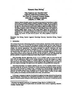
To test the effect of the warping window size to the classification accuracies, we performed an empirical experiment on all seven classification datasets. We vary the warping window size from 0% (Euclidean) to 100% (no constraint/full calculation) and record the accuracies.
100 910 100
This finding suggests that warping window size adjustment does affect accuracy, and that the effect also depends on the database size. This in turn suggests that we should find the best warping window size on realistic (for the task at hand) database sizes, and not try to generalize from toy problems. To summarize, there is no evidence to support the idea that we need to be able to support wider constraints. While it is possible that there exist some datasets somewhere that could benefit from wider constraints, we found no evidence for this in a survey of more than 500 papers on the topic. More tellingly, in spite of extensive efforts, we could not even create a large synthetic dataset for classification that needs more than 10% warping.
20
40
60
80
100
99
95
98
90
97
Leaf
85
Control Chart
96 80 95 75
94
70 65 0 100
93 20
40
60
80
100
92 0
20
40
60
80
100
100
99.9
Since we have shown in Section 2 that reinterpolation of time series into the same length is at least as good as (or better than) using the original variable-length time series, we linearly interpolate all variable-length datasets to have the same length of the longest time series within the dataset and measure the accuracy using the 1-nearest-neighbor with leaving-one-out classification method. The results are shown in Figure 2. As we hypothesized, wider warping constraints do not always improve the accuracy, as commonly believed [22]. More often, the accuracy peaks very early at much smaller window size (average = 4%). We also did an additional experiment, where half of the objects in the databases were randomly removed from the database iteratively. We measure the classification accuracies for each database size; as the database size decreases, the classification accuracy also declines and the peak appears at larger warping window size.
Gun
95
94.5
99.8
99.8
99.7 99.6
Trace
99.6 99.5
Two-Pattern
99.4
99.4 99.2
99.3 99.2
99 99.1 99 0
20
40
60
80
100
0
20
40
60
80
100
99
98.5
98
Wordspotting
97.5
97
96.5
96 0
20
40
60
80
100
Figure 2. The classification accuracies for all warping window sizes (0% to 100%). All accuracies peak at very small window sizes.
All the evidence suggests that narrow constraints are necessary for accurate DTW, and the “need” to support wide (or no) constraints is just a myth.
4
Can DTW be further Speeded up?
Smaller warping windows speed up the DTW calculations simply because there is less area of the warping matrix to be searched. Prior to the introduction of lower bounding, the amount of speedup was directly proportional to the width of the warping window. For example, a nearest neighbor search with a 10% warping constraint was almost exactly twice as fast as a search done with a 20% window. However, it is important to note that with the introduction of lower bounding based on warping constraints (i.e. 4S), the speedup is now highly nonlinear in the size of the warping window. For example, a nearest neighbor search with a 10% warping constraint may be many times faster than twice a search done with a 20% window.
The amount of pruning we should actually expect depends on the lower bounds. For example, if we used a trivial lower bound hard-coded to zero (pointless, but perfectly legal), then line 4 of Table 1 would always be true, and we would have to do DTW for every pair of sequences in our dataset. In this case, amortized percentage of the warping matrix that needs to be accessed for each sequence in our database would exactly be the area inside the warping window. If, on the other hand, we had a “magic” lower bound that returned the true DTW distance minus some tiny epsilon, then line 4 of the Table 1 would rarely be true, and we would have to do the full DTW calculation only rarely. In this case, the amortized percentage of the warping matrix that needs to be accessed would be very close to zero. We measured the amortized cost for all our datasets, and for every possible warping window size. The results (and its 0-10% warping zoom-in) are shown in Figure 3. The results are surprising. For reasonably large datasets, simply using a good lower bound insures that we rarely have to use the full DTW calculation. In essence, we can say that DTW is effectively O(n), and not O(n2), when searching large datasets. For example, in the Gun, Trace, and 2-Pattern problems (all maximum accuracy at 3% warping), we only need to do
Face Gun Leaf CtrlChrt Trace 2-Pattern WordSpotting
90
80
70
50
40
30
20
10
0
Face Gun Leaf CtrlChrt Trace 2-Pattern WordSpotting
16
14
12
2
60
Amortized percentage of the O(n ) calculation required
Instead, we measure the computation time of DTW for each pair of time series in terms of the amortized percentage of the warping matrix that needs to be visited for each pair of sequences in our database. This number depends only on the data itself and the usefulness of the lower bound. As a concrete example, if we are doing a one nearest neighbor search on 120 objects with a 10% warping window size, and the 4S algorithm only needs to examine 14 sequences (pruning the rest), then the amortized cost for this calculation would be (w * 14) / 120 = 0.12*w, where w is the area (in percentage) inside the warping window constraint along the diagonal (Sakoe-Chiba band). Note that 10% warping window size does not always occupy 10% of the warping matrix; it mainly depends on the length of the sequence as well (longer sequences give smaller w). In contrast, if 4S was able to prune all but 3 objects, the amortized cost would be (w * 3) / 120 = 0.03*w.
18
100
2
To really understand what is going on, we will avoid measuring the efficiency of DTW when using index structures. The use of such index structures opens the possibility of implementation bias [9]; it is simply difficult to know if the claimed speedup truly reflects a clever algorithm, or simply care in choice of buffer size, caching policy, etc.
much less than half a percent of the O(n2) work that we would have been forced to do without lower bounding. For some of the other datasets, it may appear that we need to do a significant percentage of the CPU work. However, as we will see below, these results are pessimistic in that they reflect the small size of these datasets. Amortized percentage of the O(n ) calculation required
In spite of this, many recent papers still claim that there is a need and room for further improvement in speeding up DTW. Surprisingly, as we will show, the amortized CPU cost of DTW is essentially O(n), using trivial 4S technique.
10
8
6
4
2
0
0
10
20
30
40
50
60
Warping Window Size (%)
70
80
90
100
0
1
2
3
4
5
6
7
8
9
Warping Window Size (%)
Figure 3. (left)The amortized percentage of warping matrix that needs to be accessed during the DTW calculation for each warping window size. The use of a lower bound helps prune off numerous unnecessary calculations. (right) Zoom-in of the warping range 0-10%
If the amortized cost of DTW is linear, where does the claimed improvement from recent papers come from? It is true that these approaches typically use indices, rather than sequential search, but an index must do costly random access rather than the optimized linear scans of sequential search. In order to break even in terms of disk access time, they must avoid looking at more than 10% of the data [7], but for time series where even the reduced dimensionality (i.e. the Fourier or wavelet coefficients) is usually greater than 20 [9], it is not obvious that this is possible. Some recent papers that claim speedups credit the improved lower bounds, for example “…we present progressively tighter lower bounds… that allow our method to outperform (4S) ” [19]. Indeed, it might be imagined that speedup could be obtained by having tighter lower bounds. Surprisingly, this is not true! We can see this with our simple experiment. Let us imagine that we have a wonderful lower bound, which always returns a value that is within 1% of the correct value (more concretely, a value uniformly distributed between 99% and 100% of the true DTW value). We will call this idealized lower bound LB_Magic. In contrast, the current best-known lower bounds typically return a value between 40% and 60% of the true value [6]. We can compare the speedup obtained by LB_Magic with the current best lower bound, LB_Keogh [6], on 1-nearest neighbor search. Note that we have to cheat for LB_Magic by doing the full DTW calculation then assigning it a value up to 1% smaller. We will use a warping constraint of 5%, which is about the mean value for the best accuracy (cf. Sect. 3). As before, we measured the amortized percentage of the warping matrix that needs to be accessed for each sequence in our database. Here, we use a randomwalk data
10
6
Once again, the results are very surprising. The idealized LB_Magic allows a very impressive speedup; for the largest size database, it eliminates 99.997% of the CPU effort. However, the very simple lower bounding technique that has been in the literature for several years is able to eliminate 99.369% of the CPU effort! The difference is not quite so dramatic for very small datasets, say less than 160 objects. But here we can do unoptimized search in much less than a hundredth of a second. Note that we obtain similar results for other datasets.
[2]
Amortized percentage of the O(n2) calculations required
of length 128 data points, and vary the database size from 10 objects to 40,960 objects. Figure 4 shows the results.
10
[1]
[3] [4]
[5] [6]
9 8
No Lower Bound LB_Keogh
7
LB_Magic
[7]
6 5
[8]
4 3
[9]
2 1 0
4 2 10 20 40 80 160 320 640 128 256 512 102 40 0480 0960 0 0 0
[10]
Size of Database (Number of Objects)
Figure 4. Amortized percentage of the warping matrix that needs to be accessed. As the size of the database increases, the amortized percentage of the warping matrix accessed becomes closer to zero.
To summarize, for problems involving a few thousand sequences or more, each with a few hundred data points, the “significant CPU cost of DTW” is simply non-issue (as for problems involving less than a few thousand sequences, we can do them in less than a second anyway). The lesson for the data mining community from this experiment is the following; it is almost certainly pointless to attempt to speed up the CPU time for DTW by producing tighter lower bounds. Even if you could produce a magical lower bound, the difference it would make would be tiny, and completely dwarfed by minor implementation choices.
[11]
[12]
[13]
[14]
[15]
[16]
[17]
5
Conclusions and Future Work
In this work, we have pointed out and investigated some of the myths in Dynamic Time Warping measure. We empirically validated our three claims. We hope that our results will help researchers focus on more useful problems. For example, while there have been dozens of papers on speeding up DTW in the last decade, there has only been one on making it more accurate [15]. Likewise, we feel that the speed and accuracy of DTW that we have demonstrated in this work may encourage researchers to apply DTW to a wealth of new problems/domains.
[18]
[19] [20]
[21]
[22]
References Aach, J. & Church, G. (2001). Aligning gene expression time series with time warping algs. Bioinformatics(17), 495-508. Berndt, D. & Clifford, J. (1994). Using dynamic time warping to find patterns in time series. AAAI Workshop on Knowledge Discovery in Databases, pp. 229-248. Bozkaya, T, Yazdatani, Z, & Ozsoyoglu, Z.M. (1997). Matching and Indexing Sequences of Different Lengths. CIKM Caiani, E.G., Porta, A., Baselli, G., Turiel, M., Muzzupappa, S., Pieruzzi, F., Crema, C., Malliani, A., & Cerutti, S. (1998). Warped-average template technique to track on a cycle-by-cycle basis the cardiac filling phases on left ventricular volume. IEEE Computers in Cardiology, pp. 73-76. Cardle, M. (2003). Music-Driven Animation. Ph.D. Thesis, Cambridge University. Keogh, E. (2002). Exact indexing of dynamic time warping. In 28th VLDB. Hong Kong. pp. 406-417. Keogh, E., Chakrabarti, K., Pazzani, M., and Mehrotra, S. (2001). Locally adaptive dimensionality reduction for indexing large time series databases. SIGMOD, pp. 151-162. Keogh, E. & Folias, T. (2002) The UCR Time Series Data Mining Archive. [http://www.cs.ucr.edu/ ~eamonn/TSDMA] Keogh, E. & Kasetty, S. (2002). On the Need for Time Seires Data Mining Benchmarks: A Survey and Empirical Demonstration. In the 8th ACM SIGKDD, pp. 102-111. Kim, S.W., Park, S., & Chu, W.W. (2004). Efficient processing of similarity search under time warping in sequence databases: an index-based approach. Inf. Syst. 29(5): 405-420. Kornfield, E.M, Manmatha, R., & Allan, J. (2004). Text Alignment with Handwritten Documents. 1st Int’l workshop on Document Image Analysis for Libraris (DIAL), pp. 195-209. Laaksonen, J., Hurri, J., and Oja, Erkki. (1998). Comparison of Adaptive Strategies for On-Line Character Recognition. In proceedings of ICANN’98, pp. 245-250. Park, S.,, Chu, W, Yoon, J., and Hsu, C (2000). Efficient searchs for similar subsequences of different lengths in sequence databases. In ICDE-00. Rabiner, L., Rosenberg, A. & Levinson, S. (1978). Considerations in dynamic time warping algorithms for discrete word recognition. IEEE Trans. Acoustics Speech, and Signal Proc., Vol. ASSP-26, pp. 575-582. Ratanamahatana, C.A. & Keogh, E. (2004). Making Time-series Classification More Accurate Using Learned Constraints. SDM International conference, pp. 11-22. Ratanamahatana, C.A. & Keogh, E. (2004). Everything You Know about Dynamic Time Warping is Wrong. SIGKDD Workshop on Mining Temporal and Sequential Data. Rath, T. & Manmatha, R. (2003). Word image matching using dynamic time warping. CVPR, Vol. II, pp. 521-527. Sakoe, H. & Chiba, S. (1978). Dynamic programming algorithm optimization fro spoken word recognition. IEEE Trans. Acoustics, Speech, & Signal Proc, ASSP-26, 43-49. Shou, Y., Mamoulis, N., and Cheung, D.W. Efficient Warping of Segmented Time-series, HKU CSIS Tech rep, TR-2004-01 Tomasi, G., van den Berg, F., & Andersson, C. (2004). Correlation Optimized Warping and DTW as Preprocessing Methods for Chromatographic Data. J. of Chemometrics. Wong, T.S.F & Wong, M.H. (2003). Efficient Subsequence Matching for Sequences Databases under Time Warping. IDEAS. Zhu, Y. & Shasha, D. (2003). Warping Indexes with Enve-lope Transforms for Query by Humming. SIGMOD, 181-192.