K. Zahn, G. Maret, C. Ruà and H.H. von Grünberg. Universität Konstanz ..... tribution functions based on the MC-data (solid lines in. Fig. (4)) and on the ...
Three-Particle Correlations in Simple Liquids K. Zahn, G. Maret, C. Ruß and H.H. von Gr¨ unberg
arXiv:cond-mat/0305176v2 [cond-mat.soft] 18 Jul 2003
Universit¨ at Konstanz, Fachbereich Physik, P.O.B. 5560, 78457 Konstanz, Germany (Dated: February 2, 2008) We use video microscopy to follow the phase-space trajectory of a two-dimensional colloidal model liquid and calculate three-point correlation functions from the measured particle configurations. Approaching the fluid-solid transition by increasing the strength of the pair-interaction potential, one observes the gradual formation of a crystal-like local order due to triplet correlations, while being still deep inside the fluid phase. Furthermore, we show that in a strongly interacting system the BornGreen equation can be satisfied only with the full triplet correlation function but not with threebody distribution functions obtained from superposing pair-correlations (Kirkwood superposition approximation). PACS numbers:
Our current understanding of the structure of simple fluids is based on the n-body distribution functions g (n) , measuring the probability density of finding two, three, and more particles at specified positions in space. When the total potential energy of a liquid is given by a sum of pair-potentials, all of its thermodynamic properties can be calculated by means of the pair-correlation function g(r) ≡ g (2) (r) and its density (ρ) and temperature (T ) derivatives. However, the latter two quantities, ∂g(r)/∂ρ and ∂g(r)/∂T , explicitly depend on the triplet correlation function, even if the particle interactions are only pair-wise additive [1]. Explicit knowledge of triplet correlations is also required in perturbation theories for static fluid properties [2], in theories of transport properties [3], of solvent reorganization processes around solutes [4], of systems under shear-flow [5], but also to understand the structural properties of a 2D amorphous system [6]. Most of our knowledge on triplet correlations come from computer simulation studies of hard-spherefluids [7], Lennard-Jones fluids [8, 9] and electrolyte systems [10]. In the overwhelming majority, these papers are concerned with testing Kirkwood’s superposition approximation (KSA) [11] for the triplet distribution function. By contrast, semi-analytical theories for g (3) beyond the KSA are rather rare [9, 12]. However, despite the long-standing theoretical interest in its properties, it has never been possible to measure three-particle correlations directly. Indirect ways to identify higher-order correlations in scattering data have been suggested for instance in [13]. An alternative, but also indirect way to obtain experimental information on g (3) is based on the relationship between the isothermal pressure derivative of the fluid structure factor ∂S(q)/∂P and the triplet distribution function [1], a relationship which has been systematically exploited by Egelstaff and co-workers in rare-gas systems [14]. The present Letter reports on the first direct measurement of g (3) in a two-dimensional colloidal model liquid with well-defined pair-interaction potentials. The preparation of the samples and the experiments
FIG. 1: A typical image (500 × 380 µm) of our twodimensional colloidal model system with paramagnetic colloids of d = 4.7µm diameter. The particles interact via a potential ∼ Γ/r 3 in which the interaction strength Γ can be conveniently varied through the external magnetic field.
have been carried out as described in [15]: Spherical colloids (diameter d = 4.7 µm) are confined by gravity to a water/air interface whose flatness can be controlled within less than a micron. The field of view has a size of 520 × 440 µm containing typically about 103 particles. The particles are super-paramagnetic due to Fe2 O3 doping. A magnetic field B applied perpendicular to the air/water interface induces in each particle a magnetic moment M = χB which leads to a repulsive dipole-dipole √ pair-interaction energy of βu(r) = Γ/( πρr)3 with the interaction strength given by Γ = β(µ0 /4π)(χB)2 (πρ)3/2 (β = 1/kT the inverse temperature, χ the susceptibility). This is the only relevant contribution to the interparticlepotential which is hence conveniently and reversibly adjustable by the external field B. A typical snapshot of our system is given in Fig. (1). Γ is the only parameter determining the phase-behavior of the system: for Γ < 57 the system is liquid, for Γ > 60 it is solid, and in between, i.e. for 57 < Γ < 60, it shows a hexatic phase [15].
2
w
(3)
(3)
(r1 ) + w
(2)
(r2 ) + w
(2)
(r3 ) − ln G/β (1) with w(2) and w(3) being the two- and three-particle potential of mean force, respectively. The equation shows that − ln G ≡ β∆w(3) plays the role of a three-body potential, measuring the (extra correlation) energy of three correlated particles relative to the energy of superposed correlated pairs of particles. In an homogeneous, isotropic system, g (3) depends on only three independent variables, chosen here to be r = |r1 − r2 |, s = |r2 − r3 | and t = |r1 − r3 |. Fig. (2) shows three-particle distribution functions in the equilateral triangle geometry for all three Γ’s considered. To allow comparison with the radial distribution function p 3 (3) (r, r, r) so that g(r) we have taken the cubic root g q 3
(r1 , r2 , r3 ) = w
(2)
gSA (r, r, r) = g(r). It is evident that the KSA, while working satisfactorily at low Γ, fails to reproduce the finestructure of the triplet distribution function at higher values of Γ. Obviously, correlations beyond the level of pair-correlations become important at higher Γ. To visualize g (3) in two dimensions, r is fixed in the following to √ (2) the distance rmax where g(r) has its first peak (≈ 1/ ρ), (2) so that g (3) (rmax , s, t) varies just with s = s(x, y) and t = t(x, y) and can thus be plotted in the (x, y)-plane in form of a contour-plot. This is done in Fig. (3) for the Γ = 46 measurement. We show in the left half of (3) the figure gSA and contrast it to the full three-particle distribution function g (3) , plotted in the right half of (2) the figure. g (3) approaches g(rmax ) for large values of 2 2 x + y . To keep the figure as clear as possible, we plot-
4
Γ= 4 1/3
(3)
1/3
(2)
= g (r)
1/3
g (r,r,r)
Γ = 14 2
(2)
(3)
(3)
g SA(r,r,r)
3
g (r) , g (r,r,r)
We here analyze three different Γ(Γ = 4, 14, 46), where the system is deep in the liquid phase, and use for each (well equilibrated) system about 200 statistically independent configurations with approximately 500 particles, recorded using digital video-microscopy with subsequent image-processing on the computer. From the measured particle configurations, g (3) is obtained by computing the average count per configuration of a particular kind of triplet, divided then by the appropriate normalizing factor. Details of this calculation will be given elsewhere [16]. Triplet correlations can be characterized by the ratio between the full triplet distribution function g (3) (3) and its approximated form based on the KSA gSA = g(r1 )g(r2 )g(r3 ). This ratio is given by what is called the triplet correlation function, denoted here by (3) G(r1 , r2 , r3 ). Thus, g (3) = gSA G. All pair correlations in (3) g (3) are included in gSA , while the extent of the intrinsic correlations due to the simultaneous presence of a triplet of particles at positions r1 , r2 , r3 is quantified through the function G, which thus defines the local structure of the fluid beyond that expressed by the pair-correlation (3) functions. Introducing βw(m) = − ln g (m) , g (3) = gSA G transforms into
1
Γ = 46 0 0
1
2
3
1/2
rρ
FIG. 2: Triplet distribution functions g (3) as a function of the side length of an equilateral triangle, as computed from (3) measured particle configurations for different Γ. gSA is the triplet distribution function in the Kirkwood q superposition
approximation which on taking the cubic root, becomes the radial distribution function g(r).
(2)
3
(3)
(3)
gSA (r, r, r),
(2)
ted just those parts of g (3) − g(rmax ) and gSA − g(rmax ) that are larger than zero. The stripes that can be seen especially close to the x-axis result from the transformation g (3) (rmax , s, t) to g (3) (rmax , x, y) and appear due to limited statistics. A hexagonal lattice with a lattice con(2) stant a = rmax is superposed. Both distributions g (3) and (3) gSA reveal that the neighbors of the two central particles have positions which show a certain correspondence to the crystalline lattice points. However, while the banana(3) like structure of gSA reflects just the coordination shells of the lattice, the full distribution function g (3) shows a well-developed, angular dependent substructure, with individual peaks for every lattice point in the first coor(3) dination shell. Fig. (4) shows g (3) and gSA of Fig. (3) (2) (2) along the line (r = rmax , s = rmax , t = t(φ)), which is a (2) circle of radius rmax around the right particle in Fig. (3), passing through all lattice points of the particle’s first coordination shell (arrows in Fig. (4) mark positions of lattice points). It can be clearly seen that g (3) develops
(r max, rmax, t(φ)) , g (rmax, rmax, t(φ))
(1/3)
3
2.5
(2)
40
3
y x
r
0
(3) (2)
20
φ
s
t
(2)
-20
-60
-40
-20
(2)
φ (2) rmax
(3) 0
20
g (3) SA
40
g
60
(3)
(2)
FIG. 3: Distribution functions g (3) (r = rmax , s(x, y), t(x, y)) (3) (2) (right half of the figure) and gSA (r = rmax , s(x, y), t(x, y)) (left half of the figure) in the (x, y)-plane (Γ = 46). The missing half of each distribution is just the mirror-image of (2) the one actually plotted. The constant g(rmax ) is subtracted from the distributions and only positive values are plotted with a grey-level scheme between white (zero) and black (max. value).
rmax
(3)
gSA
Γ = 46
(3)
g
1.5 1
(3)
ΓΓ= =4 4 1414 4646
0.5
(2)
ρ
β∆w
(2) ~ 1/ rmax
-40
2
t( φ)
0
-lnG=β∆w
(3)
-lnG=β∆w -0.5 0
60 (3)
φ
120
180 (2)
FIG. 4: g (3) and gSA from Fig. (3) for fixed values of r = rmax (2) and s = rmax , as a function of the angle φ (see inset). Symbols (solid lines) for distributions generated from measured (MCsimulated) configurations. Also given is the logarithm of the triplet correlation function G, which is related to the triplet correlation energy ∆w(3) , for Γ = 4 (dashed line), Γ = 14 (dashed-dotted line) and Γ = 46 (dashed line).
(3)
peaks at the lattice points while gSA completely fails to reflect the hexagonal structure. Also given is the function − ln G, i.e. ∆w(3) , of eq. (1), now for all three values of Γ studied here. It is evident how ∆w(3) gradually forms on increasing Γ, with values up to one kT (in other regions of the (r, s, t)-space we find energies as high as 4 kT !). It is also seen that the regions of attractive and repulsive correlation energies ∆w(3) correspond to the correcting (3) effect which the function G has on gSA to ensure that g (3) adapts locally to the hexagonal symmetry. We conclude that it is an effect entirely due to three-particle correlations, i.e. due to the function G, which is responsible for the observed formation of a crystal-like local environment around particles well below the freezing transition. We also performed Monte-Carlo (MC) simulations using √ the above-given pair-potential βu(r) = Γ/( πρr)3 (with a better statistic than in the experiment: 500 configurations with 2000 particles, periodic boundary conditions). The almost perfect agreement between the distribution functions based on the MC-data (solid lines in Fig. (4)) and on the experimental configurations (symbols in Fig. (4)), demonstrates that our model liquid consists of particles interacting solely via pair-wise additive and precisely known potentials. Furthermore, we carried out MC simulations for the solid phase (Γ = 80), starting from a perfect hexagonal lattice, and compared the resulting triplet distribution function with the experimental one for the Γ = 46
measurement in the liquid phase, see [16]. The distributions look quite similar: as regards the correlations between the central pair and the first coordination shell (in a plot like that in Fig. (3)), there is hardly any difference between the liquid and the solid phase. Pronounced differences are observable, however, in the second shell: in the liquid phase the next nearest neighbors are broadly distributed midway between adjacent lattice nodes (see Fig. (3)), while the Γ = 80 distribution correlates much better with the lattice structure. However, even for Γ = 80 this correspondence is far from perfect; it is well developed along the y-direction, but becomes worse on increasing φ to 180◦ where there is still an extended smeared-out distribution showing no clear preference for certain lattice points. Clearly, approaching T → 0 (Γ → ∞), one will ultimately observe peaks in g (3) positioned exclusively on the lattice points. We should remark that in three dimensions a similar correspondence between the peaks in g (3) and an underlying crystal lattice should be much harder to find. In 3D, every triplet of particle lies, of course, also in a plane, and can accordingly be plotted as in Fig. (3). However, then there is not one, but a superposition of many possible lattice planes that one has to compare this distribution with. To demonstrate that triplet correlations are significant not only locally, but also when integrated over the whole
4 Acknowledgment: We are grateful to Gerd Haller for providing the photograph of the sample in Fig. (1).
lhs of eq. 2
30
(3)
rhs of eq. 2 with g
(3)
β (w`(r) - u`(r)) / ρ
1/2
rhs of eq. 2 with gSA
20
Γ = 46
10
0
-10
Γ=4
1
2 1/2 rρ
3
FIG. 5: Test of Kirkwood’s approximation using experimentally determined three-particle distribution functions (Γ = 46 and Γ = 4). Solid lines for the left hand side of the BornGreen equation (eq. 2), symbols for the right hand side, evaluated using the full triplet distribution function g (3) (crosses) (3) and the distribution function gSA (open circles) which is based on Kirkwood’s superposition approximation.
volume we consider the Born Green equation [17], ∂w(2) (r12 ) ∂u(r12 ) − =ρ ∂r1 ∂r1
∂u(r13 ) g (3) (r1 , r2 , r3 ) dr3 , ∂r1 g(r12 ) (2) relating the difference between the mean force and the direct pair-force to an integral over the force on particle 1 due to a third particle at r3 , weighted by the probability ρg (3) dr3 /g(r12 ) of finding this particle in dr3 at r3 when it is known that other particles are located at r1 and r2 . This equation is exact if pairwise interactions can be assumed. To illustrate the importance of three-particle correlations, we numerically computed the right-hand side of eq. (2) using both the full and the approximated triplet (3) function, g (3) and gSA , of the Γ = 4 and Γ = 46 measurement and compared it in Fig. (5) to the left-hand side of eq. (2), evaluated using u(r) and g(r). For the strongly interacting system (Γ = 46) the KSA fails completely. Three-particle correlations are thus seen to be important not only to obtain locally the correct structure, but also to obtain globally the correct difference between mean and direct force via the Born-Green equation. Z
[1] P. Schofield, Proc. Phys. Soc. 88, 149 (1966). [2] G. Stell, J.C. Rasaiah, and H. Narang, Mol. Phys. 27, 1393 (1974); W.G. Madden, D.D. Fitts, and W.R. Smith, Mol. Phys. 35, 1017 (1978); C.G. Gray, K.E. Gubbins, and C.H. Twu, J. Chem. Phys. 69, 182 (1978). [3] K. Scherwinski, Mol. Phys. 70, 797 (1990). [4] T. Lazaridis, J. Phys. Chem. B 104, 16 (2000). [5] H.Wang, M.P.Lettinga, and J.K.G. Dhont, J.Phys.: Condens. Matter 14, 7599 (2002); J.K.G. Dhont and G. N¨ agele, Phys. Rev. E 58, 7710 (1998). [6] H. K¨ onig, to be published [7] B.J. Alder, Phys. Rev. Lett. 12, 317 (1964); E.A. Muller and K.E. Gubbins, Mol. Phys. 80, 11 (1993). [8] A. Rahman, Phys. Rev. Lett. 12, 575 (1964); S. Gupta, J.M. Haile, and W.A. Steele, Chem. Phys. 72, 425 (1982); J.A. Krumhansl and S.S. Wang, J. Chem. Phys. 56, 2034 (1972); J.A. Krumhansl and S.S. Wang, J. Chem. Phys. 56, 2179 (1972); S.S. Wang and J.A. Krumhansl, J. Chem. Phys. 56, 4287 (1972); H.J. Raveche, R.D. Mountain, and W. B. Streett, J. Chem. Phys. 61, 1970 (1974); H.J. Raveche and R.D. Mountain, in Progress in liquid physics, edited by C.A. Croxton (Wiley, New York, 1978); [9] W.J. McNeil, W.G. Madden, A.D.J. Haymet, and S.A. Rice, J. Chem. Phys. 78, 388 (1983). [10] P. Linse, J. Chem. Phys. 94, 8227 (1991); Y.Tananka and Y. Fukui, Prog. Theor. Phys. 53, 1547 (1975); S. Jorge, E. Lomba, and J.L.F. Abascal, J. Chem. Phys. 117, 3763 (2002). [11] J.G. Kirkwood, J. Chem. Phys. 3, 300 (1935). [12] S.A. Rice and J. Lekner, J. Chem. Phys. 42, 3559 (1965); R.N. Sane, Phys. Rev. A 25, 1779 (1982); P. Attard, J. Chem. Phys. 95, 10 (1991); M. Fushiki, Mol. Phys. 74, 307 (1991). [13] S. Dietrich and W. Fenzl, Phys. Rev. B 39, 8873 (1989). [14] D.J. Winfried and P.A. Egelstaff, Can. J. Phys. 51, 1965 (1973); P.A. Egelstaff, D.I. Page, and C.R.T. Heard, Phys. Lett. A 30, 376 (1969); W. Montfrooij, L.A. de Graaf, P.J. van der Bosch, A.K. Soper, and W.S. Howells, J.Phys.: Condens. Matter 3, 4089 (1991);P.A. Egelstaff, Ann. Rev. Phys. Chem. 24, 159 (1973). [15] K. Zahn, R. Lenke, and G. Maret, Phys. Rev. Lett. 82, 2721 (1999); K. Zahn and G. Maret, Phys. Rev. Lett. 85, 3656 (2000). [16] C. Ruß, K. Zahn and H.H. von Gr¨ unberg, submitted to J. Phys. Cond.Mat. (2003). [17] M. Born and H.S. Green, Proc. R. London Soc. Ser. A 188, 10 (1946); J. Yvon, Actualities Scientifiques et Industriel 203, 1 (1935).


![[PDF] Theory of Simple Liquids, Third Edition Popular ... - Google Sites](https://m.moam.info/img/260x300/pdf-theory-of-simple-liquids-third-edition-popular_6478f23a097c474d228db729.jpg)