Threshold and Symmetric Functions Over Bitmaps

arXiv:1402.4073v1 [cs.DB] 17 Feb 2014

Threshold and Symmetric Functions Over Bitmaps TR-14-001, Dept of CSAS Daniel Lemire Owen Kaser LICEF, TELUQ Dept. of CSAS Université du Québec UNBSJ Montreal, QC Saint John, NB February 18, 2014

Threshold and symmetric functions over bitmaps Owen Kaser and Daniel Lemire February 18, 2014

Abstract Bitmap indexes are routinely used to speed up simple aggregate queries in databases. Set operations like intersections, unions and complements can be represented as logical operations (and, or, not). However, less is known about the application of bitmap indexes to more advanced queries. We want to extend the applicability of bitmap indexes. As a starting point, we consider symmetric Boolean queries (e.g., threshold functions). For example, we might consider stores as sets of products, and ask for products that are on sale in 2 to 10 stores. Such symmetric Boolean queries generalize intersection, union, and T-occurrence queries. It may not be immediately obvious to an engineer how to use bitmap indexes for symmetric Boolean queries. Yet, maybe surprisingly, we find that the best of our bitmap-based algorithms are competitive with the state-ofthe-art algorithms for important special cases (e.g., MergeOpt, MergeSkip, DivideSkip, ScanCount). Moreover, unlike the competing algorithms, the result of our computation is again a bitmap which can be further processed within a bitmap index. We review algorithmic design issues such as the aggregation of many compressed bitmaps. We conclude with a discussion on other advanced queries that bitmap indexes might be able to support efficiently.

1

Introduction

There are many applications to bitmap indexes, from conventional databases (e.g., Oracle [3]) all the way to information retrieval [9] and including on column stores [35]. We are primarily motivated by the application of bitmap indexes to common databases (i.e., row stores). In this case, it has long been established that bitmap indexes can This report is intended to be viewed electronically and uses fonts and colours that make it unsuited for viewing on paper.

1

Table 1: Algorithms considered in this report. Algorithm S CAN C OUNT H ASH C NT M G O PT DS K L OOPED T REE A DD SS UM CS V C KT S RT C KT S O PC KT RBM RG W H EAP WMGSK W 2C TA W 2C T N W 2C T I W S ORT

Source [25] variant of S CAN C OUNT [33] [25] novel novel novel novel novel novel modified from [23] [33] [25] novel novel novel novel

Section § 4.2 § 4.2 § 4.3 § 4.3 § 4.5 § 4.4.2 § 4.4.2 § 4.4.2 § 4.4.1 § 4.4 § 4.1 § 4.3 § 4.3 § 4.2.2 § 4.2.2 § 4.2.2 § 4.2.1

speed up several queries corresponding, e.g., to intersections or unions (such as SELECT * WHERE A=1 AND B=2). We show that these good results extend to the more advanced queries we want to consider. Since bitmap indexes are widely used and basic Boolean operators over the bitmaps have been found useful in answering queries, our broad goal is to investigate how to integrate symmetric Boolean functions (in particular, threshold functions such as the Majority function) into the set of operations supported on bitmaps. This would permit queries that arbitrarily combine such complex functions and the standard operations permitted on bitmaps (OR, AND, XOR, perhaps NOT) and so forth. Of course, the set of basic operations (typically depending whether NOT is provided) may be sufficient to synthesize any required function, symmetric or otherwise. However, the efficiency of such approaches is not clear. To our knowledge, it has never been investigated. The concrete contribution of this report is a study of an extensive set of alternative algorithms (see Table 1) to compute threshold functions over bitmap indexes. Many of the alternatives can be generalized to handle arbitrary symmetric Boolean functions. The theoretical analyses of these alternatives are summarized in Tables 3 and 4. The notation used in the tables can be found in Table 2. We shall see that the characteristics of the bitmaps, such as the number of ones

2

or the number of distinct runs, have a major effect in determining the superior alternatives. This is determined by extensive experiments described in § 5. To obtain results that correspond to a practical applications of bitmap indexes, we focus on using threshold functions over bitmap indexes to answer similarity queries. Similarity Queries: A similarity query presents a prototypical item. We determine the criteria that this item meets, and then seek all items that meet (at least) T of these criteria. For example, if a user liked a given movie, he might be interested in other similar movies (e.g., same director, or same studio, or same leading star, or same date of release). As part of a recommender system, we might be interested in identifying quickly all movies satisfying at least T of these criteria. Similarity queries could be used to study the vocabulary of a corpus of texts. Items are vocabulary words, and the occurrence within a given text is a binary attribute. Given a word such as “pod”, we will seek words that occur in many of the same texts that “pod” occurs in. We might thus find “whale” and “pea”, besides many words that occur in almost every text. Once filtered of words that occur commonly across the corpus, we might produce information that would interest a literary analyst or linguist. Similarity queries have previously been used with approximate string matching [25, 33]. In this case, items are small chunks of text, and the occurrence of a particular q-gram is a criterion2 . In this previous work, each q-gram has a sorted list of integers that specify the chunks of text containing it. Ferro et al. [12] solve a very similar problem, but instead use a bitmap for each q-gram3 . Montaneri and Puglisi [28] extend the bitmap approach to detect near-duplicate documents arriving over time. A generalization of a similarity query presents several prototypical items, then determines the criteria met by at least one of them. We then proceed as before, finding all items in the database that meet at least T of the criteria. Another generalization allows criteria to be assigned different weights, to reflect their relative importance. In our recommender system, we might want to give more weight to having the right director than the right movie studio. Once the criteria have been defined, it is possible to use SQL to handle the rest of the query. For instance, one might use a query4 like SELECT ∗ FROM m o v i e s WHERE I F ( Lead= " Sean Penn " , 1 , 0 ) + IF ( S t u d i o =" Paramount " , 1 , 0 ) + 2

Their experiments used q = 3. Their experiments used q = 2. 4 MySQL syntax used. Some databases use IIF or CASE instead of IF. 3

3

IF ( D i r e c t o r =" Ridley S c o t t " , 1 , 0 ) > 2 Assuming you have a bitmap index, can you do better than the row-scan that would be done by a typical database engine? Formulation We take N sorted sets over a universe of r distinct values. For our purposes, we represent sets as bitmaps using r bits. See Table 2. The sum of the cardinalities of the N sets is B. We apply a threshold T (1 ≤ T ≤ N ), seeking those elements that occur in at least T sets. Because the cases T = 1 and T = N correspond to intersections and unions, and are well understood, we assume that 2 ≤ T ≤ N −1. These queries are often called T -overlap [26, 5] or T -occurrence [25, 18] queries. We show that, indeed, bitmap indexes can be used to speed up T -overlap queries (when compared with a row-store scan, see § 3). We can map a T -overlap query to a query over bitmaps using a Boolean threshold function: given N bits, the T -threshold function returns true if at least T bits are true, it returns false otherwise. A (unary) bitmap index over a table has as many bitmaps as there are distinct attribute values. Each attribute value (say value v of attribute a) has a bitmap that encodes the set of row-ids (rids) that satisfy the criterion v = a. A T -overlaps query seeks rids that occur in at least T of N chosen sets. Since each set is encoded as a bitmap, we need to compute a bitwise threshold function over the N chosen bitmaps. Threshold functions are a subset of the symmetric Boolean functions. They include the majority function: given N bits, the majority function returns true when dN/2e or more bits are true, and it returns false otherwise. We denote the processor’s native word length as W (currently5 W = 64 is typical). An uncompressed bitmap will have dr/W e words. If you have N bitmaps, then you have N dr/W e words. To simplify, we assume log N < W < r as well 6 as log r ≤ W , which would typically be the case in the applications we envision. Also, we assume that B ≥ N , which would be true if there is no empty bitmap. For the remainder of the paper we assume that a bitmap index has been created over the table, where each attribute value is represented by a bitmap (compressed or otherwise). Perhaps the index is smaller than the original table and can fit in main memory; if not, we assume that at least the N bitmaps involved in the threshold query can be simultaneously stored in memory. Thus, even if the N bitmaps must be initially loaded from disk, we only consider in-memory computation. For even larger datasets, we could assume that the table has been horizontally fragmented 5

Common 64-bit PCs have SIMD instructions that work over 128-bit (SSE and AVX) and 256-bit (AVX2) vectors. These instructions might be used automatically by compilers and interpreters. 6 In this paper, log n means log2 n.

4

Table 2: Notation used in analyses. Symbol N Nmax T r Bi B |Bi | B B0 B 00 L RUN C OUNT ϑ(T, B) ϑ(T, {b1 , . . . , bN }) W

Meaning Number of bitmaps in query Maximum value of N allowed Minimum threshold length of bitmaps (largest index covered) ith bitmap {Bi } number of P ones in ith bitmap i |Bi | number of ones not in T − 1 largest bitmaps number of ones not in L largest bitmaps number of long bitmaps reserved in DS K number of runs of zeros and ones in collection of bitmaps threshold function over bitmaps threshold function over bits bi machine word size

(the fragments would be much larger than with a row store), such that, for any fragment, any N bitmaps fit in memory. This paper does not consider external-memory algorithms that can compute thresholds without using much main memory. Lower Bound: Towards a lower bound for the problem, note if the output indicates that X entries meet the threshold, we must have processed input such that at least T X predicate-satisfaction events have been observed. If each such observation triggers Ω(1) work (as it does with S CAN C OUNT (§ 4.2), when a counter is incremented), this implies an Ω(T X) lower bound. However, this leaves open the possibility of using bit-level parallelism (readily available in bitmap inputs) to process several events per machine operation. (See § 4.4.) It also leaves open the possibility of using Run Length Encoding (RLE), whereby many consecutive events can be succinctly represented and processed together. We present such an approach later in § 4.1. While it might superficially appear that a lower-bound could be based on a need to read the entire input, note that sometimes there is no such need. For instance, suppose the threshold is T and we have already processed N − 1 of our N input bitmaps. It is only necessary to inspect the last bitmap at positions where the current count is T − 1. Other positions already achieve the threshold, or have no possibility of achieving it. The strategy of skipping portions of the input has been

5

Table 3: Time and memory complexity of some threshold algorithms over uncompressed bitmap indexes. Our memory bounds exclude storage for the input and output bitmaps. The RBM RG is based on run-length encoding and is thus omitted. Factor rN/W is required to read all the input one word at a time. We assume that rN/W  N log N . Actual bitmap libraries may detect that a bitmap has no ones past some word and thus run faster. Algorithm

Time complexity (big-Oh)

S CAN C OUNT H ASH C NT W H EAP WMGSK M G O PT DS K L OOPED T REE A DD SS UM CS V C KT S RT C KT S O PC KT W 2C T N W 2C TA W 2C T I W S ORT

rN/W + B expected rN/W + B rN/W + B log N rN/W + B log N r(N − T )/W + B 0 (log(N − T ) + T ) r(N − L)/W + B 00 (log(N − L) + L) rN T /W rN/W rN/W rN/W log2 (N )rN/W N T rN/W rN/W + BN rN/W + BN rN/W + BN rN/W + B log W N

1 2

3 4

5

Space complexity (big-Oh) horizontal vertical W r W B N N N N N −T N −T N −L N −L T rT /W N rN/W N rN/W N r log(N )/W N log2 N rN log2 (N )/W T N rN T /W WN B WN B WN B WN B

Comment

Note 1

Note 2 Note 3 Note 3 Note 3 Note 3 Note 4 Note 4 Note 5

Pruning can allow skipping portions of all bitmaps, so rN/W and B can be reduced, depending on data. While fewer than 7N temporary bitmaps are generated, register-allocation techniques would usually be able to share space between temporaries. In many cases, space for o(N ) bitmaps would suffice. Register allocation should be able to greatly reduce the actual space requirements. Pruning can reduce the amount of temporary data processed, but every input bitmap is completely scanned. W 2C T I prunes more than W 2C TA. Vertical implementation would sort B values, for a time of O(rN/W + B log B).

used in prior algorithms noted in Table 1. Theoretically, they typically assume the ability to do random access on the input, so we can jump over irrelevant portions. The sorted-list-of-integers representation facilitates this kind of action, as do uncompressed bitmaps. However, word-aligned compressed bitmap representations typically do not support the required access in constant time [40]. Nevertheless, we have been able to adapt this idea to compressed bitmaps: it may require more than constant time to skip over input, but we can do the work in a small fraction of the time it would take to process otherwise.

6

Table 4: Time and memory complexity of some threshold algorithms over RLE-compressed bitmap indexes. We assume that one can iterate over the ones in a RLE-compressed bitmap in Θ(1) time per one. Horizontal or iterator-based implementations are not considered. Algorithm S CAN C OUNT H ASH C NT W H EAP WMGSK M G O PT DS K L OOPED T REE A DD SS UM CS V C KT S RT C KT S O PC KT RBM RG W 2C T N W 2C TA W 2C T I W S ORT 1 2 3 4 5

6

Time complexity bound (big-Oh) r+B expected B + (B/T ) log(B/T ) B log N B log N B 0 (log(N − T ) + T ) + B − B 0 B 00 (log(N − L) + L) + B − B 00 N T basic bitmap operations N basic bitmap operations N basic bitmap operations N basic bitmap operations N log2 N basic bitmap ops N T basic bitmap ops RUN C OUNT log N BN BN BN B log B

Space (big-Oh) r B N N N N T bitmaps N bitmaps N bitmaps log N bitmaps N log2 N bitmaps N T bitmaps N B B B B

Comment Note 1 Note 2 Note 3 Note 3 Note 4 Note 5 Note 5 Note 5 Note 5

Note 6 Note 6

Access pattern is efficient. Access pattern is inefficient. Pruning can reduce B. Pruning can reduce B 00 and B. With register allocation, the space complexity would typically be much lower than the value shown, which merely bounds the number of temporary bitmaps created. Pruning reduces N .

2

Background

We next consider relevant background on bitmaps, Boolean functions and two major implementation approaches for bitmap operations.

2.1

Bitmaps

We consider compressed and uncompressed bitmaps. The density of a bitmap is the fraction of its bits that are ones. A bitmap with very low density is sparse, and such bitmaps arise in many applications. Uncompressed Bitmaps An uncompressed bitmap represents a sorted set S over {0, 1, . . . , r} using d(r + 1)/W e consecutive words. The W bits in the first word 7

record which values in [0, W − 1] are present in S. The bits in the second word record the values in [W, 2W − 1] that are in S, and so forth. For example, the set {1, 2, 7, 9} is represented as 10000110 00000010 with W = 8; the number of ones is equal to the cardinality of the set. Uncompressed bitmaps have the advantages of a fixed size (updates do not change the size) and an efficient membership test. However, if r is large, the bitmap occupies many words—even if it is representing a set with few elements. The Java library contains a B IT S ET class [16] which implements an uncompressed bitmap data structure. In most respects, it is an uncompressed bitmap, but it does not have a fixed size. The number of words it occupies is d(ˆ r + 1)/W e, where rˆ = max S. Note that rˆ might be much less than r; also note that if a new element larger than rˆ is inserted into S, the B IT S ET may need to grow. Not storing the trailing empty words is an optimization that would slightly complicate operations over a B IT S ET. But in the case of an AND operation between a B IT S ET representing S1 (with largest value rˆ1 ) and one representing S2 (with largest value rˆ2 ), bitwise AND instructions would only need to be done over d(min(ˆ r1 , rˆ2 ) + 1)/W e words, rather than d(r +1)/W e. Similar optimizations are possible for OR and XOR. One consequence is that the speed of an operation over B IT S ETs depends on the data involved. Compressed Bitmaps In many situations where bitmaps are generated, the processes creating the bitmaps generate long runs of consecutive zeros (and sometime long runs of ones). The number of such runs is called the RUN C OUNT of a bitmap, or of a collection of bitmaps [22]. Though there are alternatives [29], the most popular compression techniques are based on the (word-aligned) RLE compression model inherited from Oracle (BBC [3]): WAH [38], Concise [7], EWAH [23]), COMPAX [14]. These techniques typically use special marker words to compress fill words: sequences of W bits made of all ones or all zeros. When accessing these formats, it is necessary to read every word to determine whether it indicates a sequence of fill words, or a dirty word (W consecutive bits containing a mix of ones and zeros). The EWAH format supports a limited form of skipping because it uses marker words not only to mark the length of the sequences of fill words, but also to indicate the length of the sequences of dirty words. Because of this feature, it is possible to skip runs of dirty words when using EWAH. Compressed bitmaps are often appropriate for storing sets that cannot be efficiently handled by uncompressed bitmaps. For instance, consider the bitmap consisting of a million zeros followed by a million ones. This data has two runs (RUN C OUNT=2) but a million ones. It can be stored in only a few words.

8

RLE compressed bitmaps are not an efficient way to store extremely sparse data that does not have dense clusters. Sparse data with very long runs of zeros between elements will result in a marker word and a dirty word for each one bit. This would be even less efficient than explicitly listing the set elements. Software libraries for compressed bitmaps will typically include an assortment of basic Boolean operations that operate directly on the compressed bitmaps. One would expect to find operations for AND, OR, and often one finds XOR, ANDNOT, and NOT. Some libraries support only binary operations, whereas others support wide queries (for instance, a “wide” AND would allow us to intersect four bitmaps in a single operation, rather than having to AND bitmaps together pairwise). Even if intersection is eventually implemented by pairwise operations, the wide query allows the library to decide how to schedule the pair-at-a-time operations, and this may lead to a performance gain [39].

2.2

Boolean Functions and Circuits

For relevant background on Boolean functions, see Knuth’s book [21]. Boolean functions can be computed by Boolean circuits that compose some basic set of operators, such as NOT and binary AND and OR. Some Boolean functions are symmetric. These functions are unchanged under any permutation of their inputs. I.e., a symmetric function is completely determined if one knows the number of ones (the Hamming weight) in its inputs. An example symmetric function outputs 0 iff the Hamming weight of its inputs is a multiple of 2: this is the XOR function. Another example is the function that indicates whether the Hamming weight of its inputs is less than 5. The “delta” function indicates whether the Hamming weight of its inputs is some specified value, and another symmetric function indicates whether between 5 and 8 of its inputs are ones. Some Boolean functions are monotone; changing an input of such a function from 0 to 1 can never cause the output to go from 1 to 0. It is well known that the set of monotone Boolean functions equals the set of Boolean functions that can be implemented using only AND and OR operators.

2.3

Threshold Functions

Threshold functions are those Boolean functions that are both symmetric and monotone. Such a function indicates whether the Hamming weight of its inputs exceeds some threshold T . Function ϑ(T, {b1 , . . . , bN }) denotes the function that outputs 1 exactly when at least T of its N inputs are 1. Several well-known functions are threshold functions: Note that ϑ(1, {b1 , . . . , bN }) is merely a wide OR, 9

ϑ(N, {b1 , . . . , bN }) is merely a wide AND, and ϑ(dN/2e, {b1 , . . . , bN }) is the majority function. Efficient compressed bitmap algorithms for wide AND, OR and XOR have been studied before [39]. Knuth [21, 7.1.1&7.1.2] discusses threshold functions and symmetric functions, as well as techniques by which general symmetric functions can be synthesized from threshold functions. There are a number of identities involving threshold functions that might be useful to a query optimizer, if thresholds were incorporated into database engines. For instance, we have that ϑ(T, {b1 , . . . , bN }) = ϑ(N − T, {¯b1 , . . . ¯bN }). If the efficiency of a threshold algorithm depends on the density of its inputs, this identity can be helpful, because it can convert very dense bitmaps into sparse bitmaps, or vice-versa. In general, threshold functions may permit weights on the various inputs. However, if the weights are positive integers, we can simply replicate input bi so that it occurs wi times. In this way we give the input an effective weight of wi . This approach may be practical if weights are small. Otherwise, the resulting threshold query may be impractically wide. Unweighted threshold functions (in the guise of T -overlap queries) have been used for approximate searching. Specifically, Sarawagi and Kirpal [33] show how to avoid unnecessary and expensive pairwise distance computations (such as editdistance computations) by using threshold functions to screen out items that cannot be approximate matches. Their observation was that strings s1 and s2 must have many (T ) q-grams in common, if they have a chance of being approximate matches to one another. Given s1 and seeking suitable s2 values, we take the set of q-grams of s1 . Each q-gram is associated with a set of the words (more specifically, with their record ids) that contain that q-gram at least once. Taking these N sets, we do a threshold function to determine values s2 that can be compared more carefully against s1 . Using q-grams, Sarawagi and Kirpal showed that T = |s1 | + q − 1 − kq will not discard any string that might be within edit distance k of s1 . In applications where k and q are small but the strings are long, this will create queries where T ≈ N.

2.4

Horizontal and Vertical Implementations

Implementations of bitmap operations can be described as “horizontal” or “vertical”. The former implementation produces its output incrementally, and can be stopped early. The latter implementation produces the entire completed bitmap. Horizontal approaches would be preferred if the output of the algorithm is to be 10

consumed immediately, as we may be able to avoid storing the entire bitmap. As well, the producer and consumer can run in parallel. Vertical implementations may be simpler and have less overhead. If the output of the algorithm needs to be stored because it is consumed more than once, there may be no substantial space advantage to a horizontal implementation. With uncompressed bitmaps, a particularly horizontal implementation exists: a word of each input is read, after which one word of the output is produced.

3

An index is better than no index

Algorithm 1 Row-scanning approach over a row store. Require: A table with D attributes. A set κ of N ≤ D attributes, and for each such attribute a desired value. Some threshold T . 1: s a set, initially empty 2: for each row in the table do 3: for for each attribute k in κ do 4: if attribute k of the row has the desired value then 5: increment counter c 6: if c ≥ T then 7: add the row (via a reference to it) to s 8: return the set of matching rows s Perhaps a simple T-occurrence query can be more effectively answered without using a bitmap index. In that case, our work would be of less value7 . Algorithm 1 shows such an approach, and Table 5 shows that it is outperformed on both compressed and uncompressed bitmaps by one of the algorithms studied (S CAN C OUNT, which is often outperformed by other bitmap algorithms). If D  N and the N attributes involved in the computation are scattered throughout the record, the row-scanning approach will not make good use of the memory system—few of the N important attributes will be in any given cache line. Moreover, interesting datasets often do not fit in main memory. Horizontal partitioning could be used, loading a group of rows, operating on them, then loading the next group of rows. This will still suffer from the inefficiencies inherent in row stores. It is reassuring to see that a bitmap index can answer our queries faster than they would be computed from the base table. We made 30 trials, using the first 7

Good algorithms over bitmaps would still be essential, in the event that the T-occurrence operation is required over a set of computed bitmaps, for which no corresponding table exists.

11

Table 5: Time (ms) required for queries. Top: Random attributes. Bottom: similarity query. Algorithm EWAH S CAN C OUNT B IT S ET S CAN C OUNT Row Scan (no index) EWAH S CAN C OUNT B IT S ET S CAN C OUNT Row Scan (no index)

C ENSUS I NCOME 5214 5168 21,275 15,913 16,999 23,129

K ING JAMES 10D 1017 805 5114 3590 3574 5063

104 rows of a dataset (CensusIncome, described in § 5.2) with 42 attributes. We randomly chose one value per attribute and randomly chose a threshold between 2 and 41. In Table 5 we see that using either a B ITSET or EWAH index for this query is four times better than scanning the table. The advantage persists, but is smaller, when a similarity query is done. The results are consistent if we use the first 104 rows of a 10-attribute dataset8 (K ING JAMES 10 D [37]).

4

Approaches for Threshold Functions

This report focuses on threshold functions but notes approaches that generalize easily to handle all symmetric functions. It also notes approaches that can be modified to support delta queries or interval queries.

4.1

RBM RG

Algorithm RBM RG is a refinement of an algorithm presented in Lemire et al. [23], and it works for bitmaps that have been run-length encoded. See Algorithm 2. The approach considers runs similarly to integer intervals. For each point, the set of intervals containing it is the same as the set of intervals containing its neighbour, unless the point or its neighbour begins a run. Each bitmap provides a sorted sequence of intervals. Heap H enables us to quickly find, in sorted order, those points where intervals begin (and the bitmaps involved). At such points, we calculate the function on its revised inputs; in the case of symmetric functions such as threshold, 8 The other real datasets used for experiments in § 5 had hundreds to many thousands of binary attributes; it would have been unreasonable to test a row store with them. K ING JAMES 10 D was selected because we had used it in prior work and it was derived from text data, as were the unsuitable datasets used in our experiments.

12

this can be done very quickly. As we sweep through the data, we update the current count. Whenever a new interval of ones begins, the count increases; whenever a new interval of zeros begins, the count decreases. For regions where no interval changes, the function will continue to have the same value. Assuming log L ≤ W , the new value of a threshold function can be determined in Θ(1) time whenever an interval changes. (The approach can be used with Boolean functions in general, but evaluating a Boolean function over N inputs may be required even when only one input has changed, taking more than constant time.) Every run passes through a N -element heap, giving a running time that is in O(RUN C OUNT log N ). One can implement the N required iterators in O(1) space each, leaving a memory bound of O(N ). The algorithm would be a reasonable addition to compressed bitmap index libraries that are RLE-based. We have added it to JavaEWAH library [24] as of version 0.8. As an extreme example where this approach would excel, consider a case where each bitmap is either entirely ones or entirely zeros. Then RUN C OUNT = N , and in O(N log N ) time we can compute the output, regardless of r or B. Algorithm 2 Algorithm RBM RG. INPUT: N bitmaps B1 , . . . , BN Ii ← iterator over the runs of identical bits of Bi Γ ← a new buffer to store the aggregate of B1 , . . . , BN (initially empty) γ ← the bit value determined by γ(Ii , . . . , IN ) H ← a new N -element min-heap storing ending values of the runs and an indicator of which bitmap a0 ← 0 while some iterator has not reached the end do let a be the minimum of all ending values for the runs of I1 , . . . , IN , determined from H append run [a0 , a] to Γ with value γ a0 ← a + 1 for iterator Ii with a run ending at a (selected from H) do increment Ii while updating γ let b be the new run-ending value for Ii if b exists then increase the key of the top item in H from a to b The EWAH implementation of RBM RG processes runs of clean words as described. If the interval from a0 to a corresponds to Nclean bitmaps with clean runs, of which k are clean runs of ones, the implementation distinguishes three cases: 13

1. T − k ≤ 0: the output is 1, and there is no need to examine the N − Nclean bitmaps that contain dirty words. This pruning will help cases when T is small. 2. T − k > N − Nclean : the output is 0, and there is no need to examine the dirty words. This pruning will help cases when T is large. 3. 1 ≤ T − k ≤ N − Nclean : the output will depend on the dirty words. We can do a (T − k)-threshold over the N − Nclean bitmaps containing dirty words. We process the N − Nclean dirty words as follows. If T − k = 1 (resp. T − k = N − Nclean ), we compute the bitwise OR (resp. AND) between the dirty words. Otherwise, if T − k ≥ 128, we always use S CAN C OUNT using 64 counters (see § 4.2). Otherwise, we compute the number of ones (noted β) in the dirty words. This can be done efficiently in Java since the Long.bitCount function on desktop processors is typically compiled to fast machine code. If 2β ≥ (N − Nclean )(T − k), we use the L OOPED algorithm (§ 4.5), otherwise we use S CAN C OUNT again. We arrived at this particular approach by trial and error: we find that it gives reasonable performance.

4.2

Counter-Based Approaches

The simple S CAN C OUNT algorithm of Li et al. [25] uses an array of counters, one counter per item. The input is scanned, one bitmap at a time. If an item is seen in the current bitmap, its counter is incremented. A final pass over the counters can determine which items have been seen at least T times. In our case, items correspond to positions in the bitmap. If the maximum bit position is known in advance, if this position is not too large, and if you can efficiently iterate the bit positions in a bitmap, then S CAN C OUNT is easily coded. These conditions are frequently met when the bitmaps represent the sets of rids in a table that is not exceptionally large. S CAN C OUNT and other counter-based approaches can handle arbitrary symmetric functions, since one can provide a user-defined function mapping [0, N ] to Booleans. However, optimizations are possible when more sophisticated counterbased approaches compute threshold functions. To analyze S CAN C OUNT, note that it requires Θ(r) counters. We assume N < 2W , so each counter occupies a single machine word. Even if counter initialization can be avoided, each counter is compared against T . (An alternative is to compare only after each increment [25], but since the counters achieve T in an unpredictable order, a sorting phase is required before the compressed bitmap index is constructed. In many cases, this extra overhead would be excessive.) Also, 14

the total number of counter increments is B. Together, these imply a time complexity of Θ(r + B) and a space complexity of Θ(r), for compressed bitmaps. For uncompressed bitmaps, we potentially have to wade through regions that store only zeros and do not contribute toward B. This adds an extra N r/W term to the time9 . Aside from the effect of N on B (on average, a linear effect), note that this algorithm does not depend on N . The S CAN C OUNT approach fits modern hardware well: note that the counters will be accessed in sequence, during the N passes over them when they are incremented. Given that 16 int counters fit into a typical 64-byte cache line, the performance improvement from fewer increments is likely to be small until average selectivity of aj = vj drops to values near 1/16. (Far below that value and we may find two successively accessed counters are in different cache lines. Well above it, and two successively accessed counters are likely to be in the same cache line, and we will not get a cache miss on both.) Experimentally, we found that using byte counters when N < 128 usually brought a small (perhaps 15%) speed gain compared with int counters. Perhaps more importantly, this also quarters the memory consumption of the algorithm. One can also experiment with other memory-reduction techniques: for instance, if T < 128, one could use a saturating 8-bit counter. Experimentally, we found that the gains usually were less than the losses to make the additional conditional check (needed to avoid incrementing the counter once it had achieved either T or the maximum byte values). (In the special case where T = 1, that is, when we want to compute the union, the S CAN C OUNT array could use single-bit counters. These counters would effectively be an uncompressed bitmap. Indeed, the JavaEWAH library [24] uses this observation in its OR implementation.) Based on our experimental results, the S CAN C OUNT Java implementation used in § 5 switches between byte, short and int counters based on N , but does not use the saturating-count approach. S CAN C OUNT fails when the bitmaps have extreme r values. If we restrict ourselves to bitmaps that arise within a bitmap index, this implies that we have indexed a table with an extreme number of rows. However, hashing can be employed to use an approach like S CAN C OUNT on data where r is especially large. Algorithm H ASH C NT uses a map from integers (items) to integers (their counts). We only need counters for as many distinct items as actually exist in our data (which could be at most B). In Java, we can use HashMap from the java.util package. Un9

This is easily done if one assumes an O(1) instruction to compute the number of leading zeros in a W -bit word. For instance, the x86 has a lzcnt instruction and the ARM has clz. Otherwise, there are approaches that use O(log W ) operations [36, 5.3], and it appears the OpenJDK implementation of Integer.numberOfLeadingZeros() uses such an approach. Without the log W assumption of an O(1) instruction, the term N r/W would become N r W .

15

fortunately, the constant-factor overheads in hashing are significantly higher than merely indexing an array. Also, S CAN C OUNT indexes the array of counters in N ascending passes, which should lead to good cache performance. Hashing will scatter accesses to boxed Integer objects that could be anywhere in memory. Somewhat higher-performance int-to-int hash maps are found in libraries such as GNU Trove [10]. However, hashing would still lead to random-looking accesses through a large array, and poor cache performance should be anticipated. Note also that, with compression, the output bitmap must be constructed in sorted order. Since B there can be at most B/T ones in the output bitmap, we have an O( B T log T ) cost for construction. 4.2.1

Sorting to Count

Algorithm W S ORT counts by converting each bitmap into a (presorted) list of positions, concatenating such lists, sorting the result, and then scanning to see which items are repeated at least T times in the large sorted list. If we process uncompressed bitmaps horizontally, this naïve approach may work well enough, especially given that sorting libraries are typically very efficient. In the worst case, in one horizontal step our bitmap fragments have W N ones, requiring that we use O(W N log(W N )) time to sort, and requiring O(W N ) space. Over the entire horizontal computation, we use O(B log(W N )) time. (We have that B = W N in the our worst-case scenario. But in others, W N is an upper bound on the number of ones in a horizontal step, and B is the total number of ones in all horizontal steps.) However, if we are not using horizontal computation, we unpack B data items and sort them in Θ(B log B) time. 4.2.2

Mergeable-Count structures

A common approach to computing intersections and unions of several sets is to do it two sets at a time. To generalize the idea to symmetric queries, we represent each set as an array of values coupled with an array of counters. For example, the set {1, 14, 24} becomes {1, 14, 24}, {1, 1, 1} where the second array indicates the frequency of each element (respectively). If we are given a second set ({14, 24, 25, 32}), we supplement it with its own array of counters {1, 1, 1, 1} and can then merge the two: the result is the union of two sets along with an array of counters ({1, 14, 24, 25, 32}, {1, 2, 2, 1, 1}). From this final answer, we can deduce both the intersection and the union, as well as other symmetric operations. Algorithm W 2C T N takes this approach. Given N inputs, it orders them by increasing length and then merges each input, starting with the shortest, into an accumulating total. A worst-case input would have all inputs of equal length, each

16

containing B/N items that are disjoint from any other input. At the ith step the accumulating array of counters will have Bi/N entries and this will dominate the merge for the step. The total time complexity for this worst-case input is PNcost −1 Θ( i=1 Bi/N ) = Θ(BN ). The same input ends up growing an accumulating array of counters of size B. If this algorithm is implemented “horizontally” on uncompressed bitmaps, the maximum temporary space would be bounded by the maximum number of ones that can be appear in N words of size W . Algorithms W 2C TA and W 2C T I are refinements. Although they end up reading their entire inputs, during the merging stages they can discard elements that cannot achieve the required threshold. For instance, W 2C TA checks the accumulating counters after each merge step. If there are i inputs left to merge, then any element that has not achieved a count of at least T − i can be pruned. Algorithm W 2C T I does such pruning during the merge step, rather than including elements and then discarding them during a post-processing step after merging each pair of sets. Because these two algorithms prune data during the processing, it might be advantageous to work from the small sets: this increases the probability that data will be pruned earlier. Hence we order input bitmaps by increasing cardinality and then merge each input, starting with the shortest, into an accumulating total. In many cases, this pruning is beneficial. However, it does not help much with the worst-case input, if T = 2. We cannot discard any item until the final merge is done, because the last input set could push the count (currently 1) of any accumulated item to 2, meeting the threshold.

4.3

T-occurrence algorithms for integer sets

Others [25, 33] have studied the case when the data is presented as sorted lists of integers rather than bitmaps. The initial application was with approximate search, to help discover all terms with a small edit distance to a user-supplied term. It is not clear that these techniques could be applied in a more general setting, to compute symmetric functions other than threshold functions. Specifically, we consider 1. W H EAP [33], 2. M G O PT [33], 3. W M G S K [25], 4. DS K [25]. For details of these algorithms, see the papers that introduced them. The approach essentially uses an N -element min-heap that contains one element per input, unless the input has been exhausted. Using the heap, it merges the W H EAP

17

sorted input sequences. As items are removed from the heap, we count duplicates and thereby know which elements had at least T duplicates. This approach can be used for arbitrary symmetric functions. It requires that we process the ones in each bitmap, inserting (and then removing) the position of each into an N element minheap. This determines the space bound. If the bitmap is uncompressed, we have an additional time cost of N r/W to find the B ones. The total time cost is thus O(B log N ) for compressed bitmaps and O(N r/W +B log N ) for uncompressed, done vertically. Horizontal processing does not change the time or space use. The remaining algorithms are also based around heaps, but are designed to exploit characteristics of real data, such as skew. Algorithm M G O PT sets aside the largest T − 1 bitmaps. Any item contained only in these bitmaps cannot meet the threshold. Then it uses an approach similar to W H EAP with threshold 1. For each item found, say with count t, it checks whether at least T − t instance of the item are found in the largest T − 1 bitmaps. The items checked for are an ascending sequence. If one of the largest bitmaps is asked to check whether item x occurs, and then is later asked whether item y occurs, we know that y > x. Items between x and y in the big list will never be needed, and can be skipped over without inspection. When the data is provided as a sorted list of integers, a doubling/bootstrapping binary-search procedure can find the smallest value at least as big as y without needing to scan all values between x and y. We can consider the portions skipped to have been “pruned”. As noted in § 2.1, providing random access is not a standard part of a RLEbased compressed bitmap library, although it is essentially free for uncompressed bitmaps. However, with certain compressed bitmap indexes it is possible to “fast forward”, skipping portions of the index in a limited way: JavaEWAH uses the fact that we can skip runs of dirty words (e.g., when computing intersections). It should be possible, through auxiliary data structures to skip even more effectively at the expense of memory usage [27, 32]. However, such auxiliary data structures do not always improve performance [9]. The alternative is to convert from bitmap representation to sorted array, apply the classic algorithm, then convert the result back into a bitmap. The overheads of such an approach would be expected to be unattractive. To bound the running time, we can distinguish the B − B 0 ones in the T − 1 largest bitmaps from the B 0 ones in the remaining N − T + 1 bitmaps. A heap of size O(N − T ) is made of the N − T + 1 remaining bitmaps, and O(B 0 ) items will pass through the heap, at a cost of O(1 + log(N − T )) each. As each item is removed from the heap, it will be sought in O(T ) bitmaps. With uncompressed bitmaps, this costs O(T ). With compressed bitmaps, the situation is more complicated. Because the items sought are in ascending order, the T − 1 bitmaps will each be processed 18

in a single ascending scan that handles all the searches. Each of the B − B 0 ones in the remaining bitmaps should cost us O(1) effort. Thus we obtain a bound of O(B 0 (log(N − T ) + T ) + B − B 0 ) for the time complexity of M G O PT on an compressed bitmap. With uncompressed bitmaps, we add a r(N − T )/W term that accounts for looking for the ones in the N − T + 1 smallest bitmaps, but we can deduct the B − B 0 term, as we do not need to wade through all positions in the T lists. We obtain a bound of O(r(N − T )/W + B 0 (log(N − T ) + T ). This analysis does not take fully into account the effect of pruning, because even the compressed bitmaps might be able to skip many of the B − B 0 ones as we “fast forward” through the largest T − 1 bitmaps. Since these are the largest bitmaps, if T is close to N or if the sizes (number of ones) in the bitmaps vary widely, pruning could make a large difference. This depends on the data. Algorithm W M G S K is a different modification of the heap-based algorithm. When removing copies of an item from the heap, if there are not enough copies to meet the threshold, we remove some some extra items. This is done in such a way that the extra items removed (and not subsequently re-inserted) could not possibly meet the threshold. They are pruned. Moreover, inspection of the heap yields a lower-bound on the next possible item that can meet the threshold. Each input can then be advanced to (or beyond) that item. Items skipped are pruned, and will avoid the overheads of being inspected and (especially) inserted into the heap. As with M G O PT the effectiveness of such pruning depends heavily on the characteristics of the data. Our bound for W M G S K does not reflect the improvements that pruning might bring in some cases; we use the same bounds as W H EAP. Algorithm DS K is essentially a hybrid of W M G S K and M G O PT. It uses both methods of pruning. However, rather than following M G O PT and choosing the T − 1 largest sets, it chooses the L largest sets. Parameter L is a tuning parameter, and choosing an appropriate value of L for a given threshold query is problematic. The authors suggest a heuristic approach whereby another tuning parameter µ is determined experimentally, for a given type of queries against a given dataset. From µ and the length of the longest input, an appropriate value of L can often be determined by a heuristic formula. We found this approach unsatisfactory in our experiments, as the best µ for one query against a dataset often differed substantially from the best µ for a similar query. (See § 5.8.2 for some detail on appropriate values for µ on our datasets.) The effectiveness of DS K is definitely affected by µ, though perhaps by less than a factor of five over a reasonable range of values. Choosing appropriate µ and hence L values will be a difficulty for any engineer planning to use DS K, especially if the input datasets are not available for prior analysis. Nonetheless, DS K might be considered to reflect the state-of-the-art for the T -occurrence problem, at least as it arises in approximate string searches. The running-time bound for DS K is obtained using reasoning similar to that 19

for M G O PT. If there are B − B 00 ones in the largest L bitmaps, then each of the remaining B 00 ones will pass through the heap and trigger searches in the L largest bitmaps. For uncompressed bitmaps, this will result in O(B 00 L) work for all the searches. For compressed bitmaps, it will result in O(B 00 L + (B − B 00 )) work for all the searches. For the right data, less than B − B 00 items may be scanned during the searches on compressed bitmaps, as with M G O PT. Algorithm DS K also has the pruning opportunities of W M G S K, whereby some of the B 00 ones are skipped. Thus, our running-time bound for DS K on uncompressed bitmaps is O(r(N −L)/W +B 00 (log(N −L)+L)). For compressed bitmaps, we do not have the r(N − L)/W cost to wade through the N − L smallest bitmaps, looking for ones. However, we will potentially face a cost of O(B −B 00 ) while fast-forwarding through the largest L lists. As with M G O PT, data-dependent pruning could reduce the B − B 00 term. As with W M G S K, the multiplicative B 00 factor can be reduced by data-dependent pruning. For compressed bitmaps, we end up with a bound of O(B 00 (log(N − L) + L) + (B − B 00 )). For an analysis of space, note that M G O PT and DS K partition the inputs into two groups. Regardless of group, each compressed bitmap input will have an iterator constructed for it. For uncompressed bitmaps, only the first group (small bitmaps) needs the iterator and auxiliary storage. For either kind of bitmap, the first group go into a heap that accepts one element per input. Thus we end up with a memory bound of O(N ), which can be refined to O(N − T ) (for M G O PT on uncompressed bitmaps) or O(N − L) (for DS K on uncompressed bitmaps).

4.4

Boolean synthesis

A typical bitmap implementation provides a set of basic operations, typically AND, OR, NOT and XOR, and frequently ANDNOT. Since it is possible to synthesize any Boolean function using AND, OR and NOT gates in combination, any desired bitmap function can be “compiled” into a sequence of primitive operations. One major advantage is that this approach allows us to use a bitmap library as a black box, although it is crucial that the primitive operations have efficient algorithms and implementations. Unfortunately, it is computationally infeasible to determine the fewest primitive operations except in the simplest cases. However, there are several decades of digital-logic-design techniques that seek to implement circuits using few components. Also, Knuth has used exhaustive techniques to determine the minimal-gate circuits for all symmetric functions of 4 and 5 variables ([21, Figs. 9&10, 7.1.2]). (Following Knuth, we assume an ANDNOT operation.) But Intel SSE or AVX supports AND NOT, as do several bitmap libraries (EWAH included). Specifically, Intel has the pandn and vpandn instructions; however it does not look like the 20

Table 6: Number of gates in Knuth’s minimum-gate constructions for N = 4 and N =5 T 1 2 3 4 5

N =4 3 7 7 3 –

N =5 4 not shown

9 10 4

Table 7: Number of 2-input operations for N = 4 and N = 5, Knuth’s optimal solution, our sideways-sum adder, our sorter, and the L OOPED approach T 1 2 3 4

Opt 3 7 7 –

N =4 Add Sort 11 3 9 7 11 7 – –

Loop 3 9 13 –

Opt 4 not shown

9 10

N =5 Add Sort 14 12 12 12 14 12 11 12

Loop 4 12 18 22

standard x86 instruction set has AND NOT. Results are given in Table 6 and are often significantly smaller than those we will obtain from our more general constructions. We need to be concerned with both running time and memory consumption. Based on Knuth’s exhaustive analysis, all 4-input symmetric (N = 4) functions can be evaluated in the minimum amount of memory possible for each, without increasing the number of operations[21, 7.1.2]. Knuth does not give an algorithm for minimum-memory evaluation, which is probably due to its close relationship to the known NP-hard Register Sufficiency problem[15, A11.1.P01] [34]. (We have a restricted version of Register Sufficiency—we only need to compute one output, rather than an output for each root of the expression dag. However, one could take a multi-rooted expression dag, introduce a new node x and make each (former) root become a child of x. The resulting dag has a single root, and the registers required for evaluation would not have changed from the original dag.) See Table 7 and 8 for information on a number of threshold circuits discussed later in this section. The sideways-sum adder needed 5 gates for (N = 3, T = 2) and the tree adder needed only 4. However, for all larger values of N and T , the sideways-sum adder used fewer gates. For N > 25, it used about 40% fewer gates. (Perhaps surprisingly, on B IT S ETs the dataset determined which of the two adders was fastest, as discussed in § 5.7.) The asymptotically larger sorting-based circuits 21

Table 8: Gates (i.e., operations) for adders and sorter for some larger N and T . Note how the sorter circuit behaves with T . N

T

43 85 120 323 329 330 786 786

30 12 105 14 138 324 481 776

Adders Tree S. Sum 272 192 562 398 806 580 2226 1586 2272 1620 2275 1623 5467 3905 5461 3899

Sorter 480 1216 1907 7518 9052 7549 28945 24233

indeed are larger even for modest N , although they are optimal for the N = 4 cases. Consider uncompressed bitmaps using a word size W , and assume that all logic operations take unit time. Then a logic circuit with C gates can obtain a batch of W threshold results with C operations. For instance, on a 64-bit architecture, our sorting circuit for 511 inputs uses about 15 k gates. Thus in 15,000 bitwise operations we can compute 64 threshold results, or 234 operations per result. Wording individually, it would take more binary operations than this to reduce 511 inputs to a single output. With a larger W , such as provided by SSE and AVX extensions, the advantage of this approach increases. However, this analysis ignores the fact that, given a limited number of registers, the CPU must spend some time loading bit vectors from main memory and storing intermediate results there. Note, however, that this approach is essentially horizontal, in that no more than W bits from each input, or each intermediate result, needs to stored at a time. With RLE compressed bitmaps, the primitive operations do not all have the same computational cost. For instance, consider a bitmap B1 that consists of a single long run of zeros and a bitmap B2 that contains a single long run of ones, and a bitmap B3 that contains alternating zeros and ones. The operations AND(B1 ,B3 ) and OR(B2 ,B3 ) are fast operations that do not require any copying or bitwise machine operations. However, OR(B1 ,B3 ) and AND(B2 ,B3 ) will be expensive operations—if B3 is mutable, then a copy must be made of it. We see that it is simplistic to assume a cost model based on the uncompressed lengths of the bitmaps, or one that merely counts the number of bitmap operations.

22

Sum-of-Products circuits We implemented classic un-minimized Sum-of-Products circuits to allow computation of arbitrary N -input Boolean functions over bitmaps. This became our S O PC KT algorithm. If the function is known to be monotone, negative literals can be omitted from the Sum-of-Products circuit.
Note that threshold functions are monotone; this realization of them consists of N dif
T N ferent T -input AND gates, whose results are the input to a single T -input OR gate. These approaches can result in huge circuits, and this is unavoidable: since none of the AND terms is contained within another of the AND terms, a corollary noted by Knuth [21, Corollary Q, § 7.1.1] of a result of Quine [31] implies that no other Sum-of-Products circuit for the function can be smaller.
If we replace each high-input gate by two input gates, we require N (T − T

N N 1) AND gates and T − 1 OR gates, for a total of T T − 1 gates. Comparing with Knuth’s results in Table 6, the result is optimal for N = 4 or N = 5 if T = 1, and reasonable when N = 4, T = 2 (11 gates versus 7). If T = N − 1 it requires Θ(T 2 ) gates. Experimentally, it often performs reasonably well in these
conditions, but otherwise the N factor makes the result impractical. T We also implemented techniques specialized for symmetric functions, obtaining a sorting-based algorithm, S RT C KT. We also obtain two adder-based algorithms, T REE A DD and SS UM. 4.4.1

Sorting

A sorting circuit [20, 5.3.4] for Booleans maps a N -bit Boolean input to a N -bit Boolean output, where the output is 1k 0N −k if the input had Hamming weight k. Boolean sorting circuits are usually depicted as comparator-based sorting networks, but each comparator is simply a 2-input AND operation and a 2-input OR operation [21, 7.1.1]. It is then simple to compute whether threshold T has been achieved: simply use the T th output bit from the sorting circuit. In general, for symmetric functions one could determine whether the input had exactly Hamming weight T by ANDing the T th output with the negation of the T + 1st output. (This is the delta function.) One could then OR together the appropriate collection of these ANDNOT gates to synthesize any desired symmetric function. Interval functions (to recognize whether the Hamming weight of the inputs is within an interval) are also achieved by the ANDNOT approach. There is no known general procedure to obtain a minimum-comparator sorting circuit [20, 5.3.4]. Asymptotically, the AKS construction [1] yields circuits with O(N log N ) comparators, but the hidden constants make this approach impractical. For modest size inputs, the construction used in Batcher’s Even-Odd sort is well known to use few comparators (see [20, 5.3.4.(11)]) even though asymptotically it will generate circuits of size Θ(N log2 N ). We used Batcher’s sort for our S RT C KT 23

algorithm. It requires only that the bitmap library provide 2-input AND and OR primitives. Intermediate results are frequently reused many times. 4.4.2

Adding

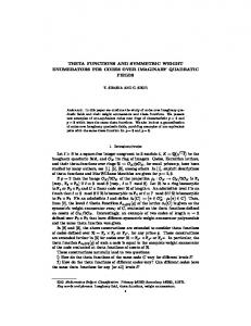
Another approach is to compute the Hamming weight of the input by summing all the input bits. We present two such approaches, and the first uses a tree of adders. (See Fig. 1.) The leaves of the tree consist of 1-bit adders (half adders, requiring an AND and an XOR operation) producing a 2-bit sum. Then these 2-bit sums are added to obtain 3-bit sums. Multi-bit adders use the ripple-carry technique, where summing two x-bit numbers uses 2x − 1 AND operations, 2x − 1 XOR operations and x − 1 OR operations. The final outcome is a log N + 1-bit binary number representing the Hamming weight of the N inputs. (When N is not a power of 2, we pad with zero inputs and then using a constant-propagation pass to simplify the resulting circuit.) This log N + 1-bit quantity is then compared to T using a ≥ circuit. Since it operates over O(log N ) inputs and N inputs involved in the Hamming weight computation, it is not crucial to have the most efficient method of computing ≥. However, if T is a power of 2, it is easy to compute the threshold function from the Hamming weight using an OR function: for instance, to see if the 4-bit number b3 b2 b1 b0 is at least 2, compute b1 |b2 |b3 . This approach can be generalized if T is not a power of two; a magnitude comparator circuit [4] can determine whether the bit-string for the Hamming weight lexicographically exceeds the bit-string for T − 1. As various designs for such circuits exist, we proceed to derive and analyze our circuit to compare a quantity to a constant. Consider two bit strings bn−1 bn−2 · · · b0 and an−1 an−2 · · · a0 , where we have n = blog 2N c. The first is greater if there is some 0 ≤ j < n where bj > aj and the two bit strings have bk = ak for all k > j. If we define prefix_match(j) = Vn−1 k=j+1 (bk ≡ ak ) then bn−1 bn−2 · · · b0 > an−1 an−2 · · · a0 can be computed as Wn−1 j=0 prefix_match(j)∧bj ∧¬aj . The prefix values can be computed with n XOR and n ANDNOT operations with prefix_match(n) = 1, prefix_match(k) = prefix_match(k + 1) ∧ ¬(bk ⊕ ak ). Altogether 5n − 1 bitwise operations (AND, ANDNOT, XOR, OR) are used to determine the truth value of the inequality bn−1 bn−2 · · · b0 > an−1 an−2 · · · a0 . We can do better because T − 1 (whose binary representation is the second bit string, an−1 · · · a0 ) is a constant. 24

• First, OR terms drop out for positions j where aj = 1, leaving us with W j|aj = 0 prefix_match(j) ∧ bj . • Second, the previous expression does not need prefix_match for the trailing ones in T − 1; they no longer appear in our expression and there is no 0 to their right. (The prefix_match value required for a 0 is indirectly calculated from prefix_match values for all positions to the left of the 0.) V • Third, we can redefine prefix_match(j) as j= 0 ; k = bs . n e x t S e t B i t ( k + 1 ) ) counts [ k ]++; scanCountAns . c l e a r ( ) ; f o r ( i n t k = 0 ; k < c o u n t s . l e n g t h ; ++k ) i f ( c o u n t s [ k ] >= K) s c a n C o u n t A n s . s e t ( k ) ;

121

SoPCkt

HashCnt

wHeap

wSort

wMgSk

wMgOpt

w2CtI

wDivSk

Looped

DSk.1

DSk.005

MgOpt

DSk.05

DSk

DSk.02

SrtCkt

ScnCnt

CSvCkt

SSum

RBMrg

TreeAdd

0.1

RBMrg

122

10

1

0.1

Figure 76: Suboptimality. PGDVD, N ≤ 32, Similarity queries. RBMrg

Looped

wHeap

wSort

CSvCkt

wMgSk

SrtCkt

wMgOpt

TreeAdd

wDivSk

DSk.005

SSum

MgOpt

w2CtI

DSk.02

DSk.1

DSk.05

DSk

ScnCnt

SoPCkt

100

SoPCkt

1000 HashCnt

Figure 75: Suboptimality. IMDB-3gr, N ≤ 32, Similarity queries.

Looped

wHeap

HashCnt

wMgSk

DSk.1

DSk.05

DSk.02

DSk.005

DSk

MgOpt

SrtCkt

wDivSk

wMgOpt

ScnCnt

wSort

CSvCkt

w2CtI

SSum

TreeAdd

(Speed - Best) / Best

(Speed - Best) / Best 1000

100

10

1

0.1

RBMrg

123

Figure 77: Suboptimality. CensusIncome, N ≤ 32, Similarity queries. wHeap

SoPCkt

wMgSk

HashCnt

wDivSk

DSk.1

wSort

DSk.05

wMgOpt

DSk.02

DSk.005

DSk

MgOpt

w2CtI

CSvCkt

ScnCnt

Looped

SrtCkt

SSum

TreeAdd

(Speed - Best) / Best 1000

100

10

1

0.1